On Infinite Separations Between Simple and Optimal Mechanisms
Abstract
We consider a revenue-maximizing seller with heterogeneous items for sale to a single additive buyer, whose values are drawn from a known, possibly correlated prior . It is known that there exist priors such that simple mechanisms — those with bounded menu complexity — extract an arbitrarily small fraction of the optimal revenue (Briest et al. 2015, Hart and Nisan 2019). This paper considers the opposite direction: given a correlated distribution witnessing an infinite separation between simple and optimal mechanisms, what can be said about ?
Hart and Nisan 2019 provides a framework for constructing such : it takes as input a sequence of -dimensional vectors satisfying some geometric property, and produces a witnessing an infinite gap. Our first main result establishes that this framework is without loss: every witnessing an infinite separation could have resulted from this framework. An earlier version of their work provided a more streamlined framework Hart and Nisan 2013. Our second main result establishes that this restrictive framework is not tight. That is, we provide an instance witnessing an infinite gap, but which provably could not have resulted from the restrictive framework.
As a corollary, we discover a new kind of mechanism which can witness these infinite separations on instances where the previous “aligned” mechanisms do not.
1 Introduction
Consider a revenue-maximizing seller with items for sale to a single additive buyer, whose values for the items are drawn from a known distribution . When , Myerson’s seminal work provides a closed-form solution to the revenue-optimal mechanism, and it has a particularly simple form: simply post a price , and let the buyer purchase the item if they please (Myerson 1981). For , however, this multi-dimensional mechanism design problem remains an active research agenda forty years later.
While simple, constant-factor approximations are known in quite general settings when is a product distribution (Chawla et al. 2007, Chawla et al. 2010, Chawla et al. 2015, Kleinberg and Weinberg 2012, Li and Yao 2013, Babaioff et al. 2014, Yao 2015, Rubinstein and Weinberg 2015, Cai et al. 2016, Chawla and Miller 2016, Cai and Zhao 2017), there may be an infinite gap between the revenue-optimal auction and any simple counterpart when values are correlated (Briest et al. 2015, Hart and Nisan 2019). More specifically: one simple way to sell items is to treat the grand bundle of all items as if it were a single item, and sell it using Myerson’s optimal auction (which sets price ). Letting denote the revenue achieved by this simple scheme, Hart and Nisan 2019 further show a connection between and any simple mechanism through the lens of menu complexity: any mechanism with menu complexity at most generates expected revenue at most .
These works establishes a strong separation between simple and optimal auctions: even when , there exist distributions such that (the optimal revenue) while . The fact that does not on its own suggest that must be “weird” (the one-dimensional distribution with CDF has this property). The “weird” property is that , which can never occur for a one-dimensional distribution.
Briest et al. 2015 and Hart and Nisan 2019 establish sufficient conditions for a distribution to satisfy . Simply put, the goal of this paper is to study necessary conditions for a distribution to satisfy . We provide two main results. The first establishes that the sufficient condition presented in Hart and Nisan 2019 is in fact necessary for (Theorem 6). The second establishes that the sufficient condition used in an earlier version of that work Hart and Nisan 2013 and Briest et al. 2015 is not necessary (Theorem 9). In establishing Theorem 9, we also construct a distribution such that yet the mechanism witnessing this provably falls outside the scope of any previous constructions (Corollary 11).
2 Preliminaries
We consider an auction design setting with a single buyer, single seller, and heterogeneous items. Note that our positive results hold for arbitrary , while our constructions use only (and is not possible). We use to denote a distribution over , the (possibly correlated) distribution over the buyer’s values for the items. The buyer is additive, meaning that their value for a set of items is equal to . We use to denote the optimal expected revenue achievable by any incentive-compatible mechanism (formally, the supremum of expected revenues, or if the supremum is undefined), and let denote the revenue achieved by selling the grand bundle as a single item using Myerson’s auction.11 1 We briefly remind the reader that serves as a proxy for the achievable revenue by any simple mechanism, especially when focusing on the gap between infinite and finite. For example, the revenue achieved by selling the items separately is at most , the revenue achieved by any deterministic mechanism is at most , and, more generally, the revenue achieved by any mechanism which offers at most distinct options is at most Hart and Nisan 2019. Finally, a mechanism is a set , where each denotes a vector of probabilities, and denotes a price. When the buyer’s valuation is , they pay the auctioneer , where .22 2 How ties are broken is irrelevant to our results — all results hold for arbitrary tie-breaking. Also, all mechanisms include an all-zero pair , to ensure individual rationality. denotes the expected revenue achieved by a particular mechanism on distribution . We will also use the shorthand to denote the allocation vector purchased by a vector , and to denote the price paid (we may drop the superscript of if the mechanism is clear from context).
Brief Overview of Hart and Nisan 2019
Below, we formally define two geometric properties of sequences of points, which are the focus of this paper. Many of the ideas below appear in both Briest et al. 2015 and Hart and Nisan 2019, but we will use the formal definitions from Hart and Nisan 2019 (and an earlier published version Hart and Nisan 2013). Below, morally the vectors correspond to possible (scaled) valuation vectors, and the vectors correspond to possible vectors of allocation probabilities.
Definition 1.
Let be an ordered sequence of points ( may be finite, or equal to ), with each . Let be another ordered sequence of points, with each , and starting with . Define the following:
We will also slightly abuse notation and define .33 3 Observe that and might be negative. Any claims made throughout this paper regarding are vacuously true when (e.g. Theorem 2). We allow to be negative to match the definition of Hart and Nisan 2019 verbatim (although our work will also show that this peculiarity of their definition is not significant).
Intuitively, is some (complicated) measure of how distinct the angles of points in are. To get intuition for this, one might try to write a short proof that when , for all (or that whenever all are parallel). We provide such a proof in Appendix A.
Still, is just some geometric measure with no obvious intuition for why this quantity should be of interest to auction designers. However, one key result of Hart and Nisan 2019 shows that this quantity has connections to simplicity vs. optimality gaps. Specifically, they show:
Theorem 2 (Hart and Nisan 2019, Proposition 7.1).
For every pair of sequences starting with , and all , there exists a distribution and mechanism such that:
Moreover, for all , the support of contains a single point of the form , for some (and no other points). Additionally, .
The “Moreover,…” portion of Theorem 2 gives some insight to their construction. Further insight can be deduced by observing that the constraint “” looks similar (but far from identical) to an incentive compatibility constraint involving a valuation vector and two allocation vectors . We refer the reader to Hart and Nisan 2019 for further details and intuition for this connection. Theorem 2 gives a framework for proving simplicity vs. optimality gaps, but of course leaves open the question of actually finding a pair of sequences . They approach this through the following observation:
Definition 3.
Given a sequence of points starting with , define (read “support gap of ”) as follows:
Observation 4.
For all , .
Finally, Hart and Nisan 2013 propose an explicit construction of a sequence with infinite SupGap.
Theorem 5 (Hart and Nisan 2013).
There exists an infinite sequence of points in such that:
Theorems 2 and 5 together yield a two-dimensional distribution with . It is also worth noting that all prior constructions follow this approach as well. For example, Briest et al. 2015 provides an infinite sequence of points in such that .
3 Our Results
Independent of Observation 4 and Theorem 5, Theorem 2 alone provides a framework for constructing distributions so that is large: find sequences so that is large. Our goal is to understand to what extent this framework is complete for constructing such instances. Our first main result establishes that any distribution with could have resulted from the framework induced by Theorem 2. Specifically:
Theorem 6.
For any distribution over items, there exists a sequence of points ( can be finite, or equal to ) , with each , such that
In particular, if , then as well.
A complete proof of Theorem 6 appears in Section 4. Observe also that because is monotone (in the sense that adding points to , anywhere, cannot possibly decrease ), the fact that is a subset of the support of (rather than the entire support) is immaterial.44 4 Of course, if the support of is uncountable, then clearly the entire support of cannot be included in . Put another way, the important aspect in constructing is how elements in the support of are ordered, rather than which points are included.
Observation 4 further provides a framework to construct sequences so that is large: construct sequences so that is large. One may then wonder if and are approximately related, for all . For this specific question, the answer is trivially no, due to incompatibility with scaling (multiplying every point in by will decrease by a factor of , but not ). Therefore, not much insight is gained by studying this precise question.
Instead, we observe that the interesting aspect of constructions resulting through is that and are aligned (that is, for some ). Specifically, even if , this equality is not maintained through the construction of Theorem 2. However, if and are aligned, this alignment property is maintained by the construction. We therefore propose the following definition, which captures the maximum value achievable by when are aligned.
Definition 7.
Let be an ordered sequence of points in ( may be finite, or equal to ). Let also be an ordered sequence of numbers, with each , starting with . Define (read ”scalar gap”) :
We will also slightly abuse notation and denote by .
Recall that we have chosen to let range in (rather than be fixed at , or ) to give potential constructions flexibility in scaling . Additionally, by ensuring that the contribution of each is non-negative, we give potential constructions flexibility to ignore points in the sequence. That is, any construction using MenuGap directly can always set , which effectively just drops from the sequence. Counting towards the objective (rather than just ) gives constructions that arise through AlignGap the same flexibility.
Lemma 8.
For all , .
The proof of Lemma 8 is in Appendix B. Lemma 8 induces a framework to design sequences with large MenuGap: design sequences with large AlignGap. Our second main result establishes that this framework is not without loss of generality, even for . Specifically:
Theorem 9.
There exist sequences such that:
A complete proof of Theorem 9 appears in Section 5. By the discussion following Definition 7, the source of this gap is entirely due to the requirement that the sequence be aligned with (and is not due to inability to scale, or inability to ignore difficult points in ). We make this crisp with the following definition and corollary, which construct a novel distribution witnessing that is provably distinct from all previous approaches.
Definition 10.
For a distribution and mechanism , define the Aligned Revenue of on :
Corollary 11.
There exist distributions over two items such that .
A proof of Corollary 11 appears in Appendix C. It is worth noting that all previous constructions establishing proceeded by producing an such that . Indeed, the Briest et al. 2015 construction provides such an when , the Hart and Nisan 2013 construction provides an when , and the Psomas et al. 2019 construction adapts parameters in that of Hart and Nisan 2013. By Theorem 2, this implies not only that , but also that . Corollary 11 establishes the existence of a fundamentally different construction,55 5 On a technical level, our construction certainly borrows several ideas from previous ones, however. as our has a finite ratio between , yet still maintains an infinite ratio between .
Additional Related Work
We’ve already discussed the most related work to ours, which is that of Hart and Nisan 2019, Briest et al. 2015. There is also a large body of work studying product distributions specifically, and establishes that simple mechanisms can achieve constant factor approximations in quite general settings Chawla et al. 2007, Chawla et al. 2010, Chawla et al. 2015, Kleinberg and Weinberg 2012, Li and Yao 2013, Babaioff et al. 2014, Yao 2015, Rubinstein and Weinberg 2015, Cai et al. 2016, Chawla and Miller 2016, Cai and Zhao 2017). Recent works have made progress in obtaining arbitrary approximations (Babaioff et al. 2017, Kothari et al. 2019), which again rely on the assumption that is a product distribution.
Three recent lines of work address the Briest et al. 2015, Hart and Nisan 2019 constructions in a different manner. First, Chawla et al. 2019, Chawla et al. 2020 consider the related buy-many model (where the auctioneer cannot prevent the buyer from interacting multiple times with the auction). Chawla et al. 2019 establishes that selling separately achieves an -approximation to the optimal buy-many mechanism in quite general settings (including the settings considered in this paper). In a different direction, Psomas et al. 2019 uses the lens of smoothed analysis (Spielman and Teng 2004) to reason about the robustness of the Hart and Nisan 2019 constructions. Finally, Carroll 2017 considers a correlation robust framework in which the valuation profile is drawn from a correlated distribution that is not completely known to the seller; the goal is to design a mechanism that maximizes the worst-case (over correlations) seller revenue, when only the items’ marginal distributions are known. Carroll 2017 shows that selling each item separately is optimal; see Bei et al. 2019, Gravin and Lu 2018 for further work in this model.
4 A Converse to Theorem 2: The Hart and Nisan 2019 Framework is WLOG
In this section, we prove Theorem 6. Our proof has two main parts. First, we will take the optimal auction for (or one that is arbitrarily close to optimal) and repeatedly simplify it through a sequence of lemmas, at the cost of small constant-factors of revenue. The second part takes this simple menu and draws a connection to MenuGap.
4.1 Simplifying the Optimal Mechanism
We show that for every , an approximately-optimal mechanism exists satisfying some useful properties. Our first step simply argues that we may ignore menu options with low prices.
Definition 12.
We say that a mechanism is -expensive if every option has price at least .
Claim 13.
For all , all distributions , and all mechanisms , there exists a -expensive mechanism satisfying .
Proof.
Take to be exactly the same as , except having removed all entries with price . For every value in the support of with in , we still have . This is simply observing that ’s favorite option in is still available in , and all options in were also available in . For any value with , we clearly have . So for all , we have , and the claim follows by taking an expectation with respect to . ∎
Our next step will show that we can assume further structure on the prices charged, at the cost of a factor of two.
Definition 14.
A -expensive mechanism is oddly-priced (respectively, evenly-priced) if for all , there exists an odd (respectively, even) integer such that .
Claim 15.
For all -expensive mechanisms , and all , there exists either an oddly-priced or evenly-priced -expensive mechanism satisfying .
Proof.
Simply let denote the set of menu options from whose price lies in for an odd integer , and denote the remaining menu options (which lie in for an even power of ). It is easy to see that is oddly-priced and is evenly-priced. Then for all , we must have . This is because ’s favorite menu option from appears in one of the two menus, and is necessarily ’s favorite option on that menu (and they pay non-zero from the other menu). Taking an expectation with respect to yields that , completing the proof. ∎
This concludes our simplification of the mechanism. In the subsequent section, we draw a connection between MenuGap and the revenue of oddly- or evenly-price -expensive mechanisms.
4.2 Connecting Structured Mechanisms to MenuGap
We begin with the following definition, which describes our proposed based on a structured mechanism for .
Definition 16 (Representative Sequences).
Let be a -expensive mechanism which is oddly-priced or evenly-priced, and let be any distribution. An -representative sequence for is the following:
- •
Define .
- •
Define offset to be if is oddly-priced, and if is evenly-priced.
- •
For all , define .
- •
For all , let be such that for all .66 6 Note that for all , such an exists, even if is not closed (as long as is non-empty). In particular, because is -expensive, we know that for all who pay . If is empty, instead omit from both lists (i.e. decrease all future indices by one).
- •
For all , let .
Proposition 17.
Let be a -expensive, and oddly- or evenly-priced. Let be an -representative sequence for . Then:
Proof.
The proof will follow immediately from two technical claims. The first claim relates and .
Claim 18.
.
Proof.
Recall that for all . Therefore, if we set a price of for the grand bundle, every would choose to purchase the grand bundle. This immediately implies the claim, as:
The second claim relates and . Crucially, this claim uses the fact that the mechanism is either oddly-priced or evenly-priced (and therefore differ by at least a factor of , for any ).
Claim 19.
If is an -representative sequence for , then .
Proof.
Recall that , and that . For any fixed , recall that because was a truthful mechanism, we must have:
The first line is simply restating incentive compatibility. The second line is basic algebra, and substituting . The third line invokes the fact that , while .
∎
With these two claims, we can wrap up the proof of Proposition 17. We can write the following:
4.3 Wrapping Up
Proposition 17, together with the fact that an oddly- or evenly-priced mechanism is guaranteed to get a good approximation to the optimum, now suffices to prove Theorem 6.
Proof of Theorem 6.
The proof will be a simple consequence of the technical lemmas in this section, once we set and appropriately. In particular, set , and . Note that -representative sequences are guaranteed to exist for any , as .
5 No Converse to Lemma 8: Separating MenuGap and AlignGap
In this section we prove our second main result: Lemma 8 does not admit a converse, even approximately. We briefly remind the reader that all previous constructions witnessing arose by establishing sequences with (in fact, even ). Theorem 9 establishes that constructions exist outside of this more restrictive framework. We now proceed with the proof of Theorem 9, beginning with a description of our sequence .
5.1 Description of our construction
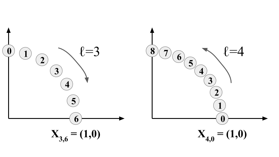
We describe our infinite sequence , which consists of consecutive layers of points, and note that this aspect of the construction is similar to that in Hart and Nisan 2013. For to , layer will have points. These points/vectors will have norm equal to one, and will be evenly spaced (in terms of their angle) between and . If is even, they will go counterclockwise from to . If is odd, they will go clockwise from to . Specifically:
- •
Define . Define .
- •
Point is the point in the layer, and is when is even, or when is odd.
- •
The infinite sequence is .
Figure 1 demonstrates two layers of our construction. In the remainder of this section, we may refer to the sequence of points by a single indexed sequence . The latter is the same as the former where points are ordered lexicographically with respect to the original indexing.
5.2 Upper Bounding via Lagrangian duality
Now that we have our construction, we first need to upper bound and establish that it’s finite. To this end, first observe that for any sequence , is the solution to the following (infinite, if is infinite) mathematical program, where the variables are (the sequence is fixed, as we’re aiming to compute ):
We next proceed with a series of relaxations of this program. Some steps are specific to our choice of from Section 5.1, while others hold for arbitrary . Our first step is specific to this construction, and simply bounds . Consider the following mathematical program:
Observation 20.
For the sequence defined in Section 5.1, .
Proof.
Every in the construction has . Therefore, the new objective function is only larger. Moreover, every in the construction has (because the norm is ), so this is relaxing the upper bound on . ∎
We will proceed to upper bound via a Lagrangian relaxation of the formulation above. Specifically, consider the following Lagrangian relaxation. We put a Lagrangian multiplier of on every constraint of the form , for all . We put a Lagrangian multiplier of on all other constraints involving . We will not put a Lagrangian multiplier on constraints binding to , and keep those in the program. This yields the following Lagrangian relaxation (for simplicity of notation below, define , and define ):
Observation 21.
For all , .
Proof.
This follows immediately from weak Lagrangian duality. For a quick refresher on weak Lagrangian duality, observe that for any feasible solution to the LP defining we must have . Therefore, for any feasible solution to the original LP, that solution is also feasible for , and the objective is only larger. Therefore, the optimal solution to must be at least as large as . ∎
We now proceed to further simplify . The next step is defined below:
Observation 22.
For all , .
Proof.
Observe that for all , . When , the maximum is achieved (and is feasible). Substituting for all concludes the proof. ∎
We make one last observation about the relaxation, which simply rewrites the objective function to group all coefficients of . For ease of notation below, define (if is finite. If , there are no notational issues).
Observation 23.
For all , .
Now, we move to analyze for our particular sequence .
Claim 24.
For the sequence defined in Section 5.1, .
Proof.
Observe here that for all , as each has norm exactly one. This means that the optimal solution for sets each . Finally, recalling that for all concludes the claim. ∎
Proposition 25.
For the sequence defined in Section 5.1, .
Proof.
Let us first observe that if is the last point in a layer, then in fact , and therefore . Therefore, these terms do not contribute to the sum. We can then rewrite the term to sum over all layers as follows:
Above, the first line follows by the reasoning in the first paragraph. The second line follows by observing that the angle between any two points in layer is exactly (and the two points in question of norm equal to one). The third line follows as for any (and all are indeed in ). The fourth line follows by substituting the definition of as a function of . The fifth line follows by definition of . The final line is just calculation for this particular infinite series.77 7 This follows as . ∎
Proposition 26.
For the sequence defined in Section 5.1, .
5.3 Step 3: Picking a to Lower Bound .
Finally, we propose a sequence and show that . We describe the sequence again in layers, to match our description of (that is, the vector corresponds to the vector ). In particular, for each even layer , the vectors will have a fixed -coordinate, and the -coordinate will increase with . For each odd layer, we will introduce no new vectors (i.e. we will just let for all in an odd layer). Specifically, the construction is as follows:
- •
Define (and note that ).
- •
Define .
- •
Define .
- •
For , define . For , define .88 8 To see that observe that for all . Therefore we get , for all (). To see that simply note that the term we subtract can’t be negative.
- •
For all even , and all , set .
- •
For all odd , and all , set .
Proposition 27.
.
Proof.
To ease notation throughout the proof, we’ll use the notation , where ( is the point on layer ). We will also use the notation if , or and (that is, if the point in the layer comes before the point in the layer). To understand , we need to understand which point “sets the gap” for , that is, which .
We first analyze which point sets the gap for (for even ; for odd the gap is zero and we don’t care which point sets it), and observe that it must either be or (that is, it must be the previous point in the same layer, or the final point in the previous even layer).
Claim 28.
For all , and all even , .99 9 For simplicity of notation, define for all .
Proof.
First, note that . Observe that the first component of is monotone increasing in (for fixed ), and the second component is monotone increasing in (for fixed ). Moreover, the second component of is , and this is the maximum possible. Also, both components of are non-negative, and therefore we conclude that whenever (in fact, this extends even to as no new are introduced in layer ). Also, whenever . ∎
Now that we know that the gap is set either by the last point in the previous layer, or the previous point in the current layer, we can nail down exactly.
Lemma 29.
For all even , and all :
Proof.
To prove the lemma, we simply compute the inner product of with the three relevant vectors . To this end, recall that:
Therefore, observe that
Similarly,
This means that no matter which point sets the gap (or if one of the points does not exist), the gap is at least . ∎
Finally, now that we know the gap for each point on an even layer, we just need to sum over each even layer.
Corollary 30.
For any even , .
Proof.
Consider the following sequence of calculations:
Above, the first line follows from Lemma 29. The second line uses the fact that , because . The third line follows as the -th harmonic sum is at least . The final line follows as . ∎
And finally, we can wrap up the proof of the proposition. Here, we just need to recall that . Therefore, we conclude that:
Above, the first line simply restates Corollary 30. The second line substitutes the definition of and . The final line follows as the indefinite integral of is (and is an absolute constant). ∎
6 Conclusion
We study the nature of distributions with . Prior work established a framework to construct such distributions, and therefore established sufficient conditions Briest et al. 2015, Hart and Nisan 2019. Our first main result establishes that the most general of these frameworks is in fact complete (Theorem 6). Our second main result establishes that the more restrictive framework, through which all previous constructions arose, is not complete (Theorem 9). Finally, we build upon our main construction to develop a novel distribution witnessing , but for which none of the “aligned” mechanisms of prior work can possibly witness this (Corollary 11).
In terms of future work, it remains open as to whether there is an alternative definition for “sequences with ” which is easier to parse. Our work establishes that understanding such sequences is necessary and sufficient to understand distributions with , and establishes that “sequences with ” is not equivalent to “sequences with .” But it would be exciting for future work to better understand sequences with .
Interestingly, ongoing work by Assadi and Schvartzman 2022 uses the framework developed in this paper in order to prove approximation results for so-called fine-grained buy-many mechanisms, a class of mechanisms which interpolates between buy-one and the recently introduced buy-many mechanisms Chawla et al. 2019, Chawla et al. 2020. In general, our techniques make it possible for future work to explore the gap between various simple versus optimal benchmarks without having to reason directly about the underlying mechanisms.
References
- [1]
- Assadi and Schvartzman [2022] Sepehr Assadi and Ariel Schvartzman. 2022. Fine-Grained Buy-Many Mechanisms Are Not Much Better Than Bundling. Manuscript from author’s website. (2022).
- Babaioff et al. [2017] Moshe Babaioff, Yannai A. Gonczarowski, and Noam Nisan. 2017. The menu-size complexity of revenue approximation. In Proceedings of the 49th Annual ACM SIGACT Symposium on Theory of Computing, STOC 2017, Montreal, QC, Canada, June 19-23, 2017. 869–877. https://doi.org/10.1145/3055399.3055426
- Babaioff et al. [2014] Moshe Babaioff, Nicole Immorlica, Brendan Lucier, and S Matthew Weinberg. 2014. A simple and approximately optimal mechanism for an additive buyer. In 2014 IEEE 55th Annual Symposium on Foundations of Computer Science. IEEE, 21–30.
- Bei et al. [2019] Xiaohui Bei, Nick Gravin, Pinyan Lu, and Zhihao Gavin Tang. 2019. Correlation-robust analysis of single item auction. In Proceedings of the Thirtieth Annual ACM-SIAM Symposium on Discrete Algorithms. SIAM, 193–208.
- Briest et al. [2015] Patrick Briest, Shuchi Chawla, Robert Kleinberg, and S Matthew Weinberg. 2015. Pricing lotteries. Journal of Economic Theory 156 (2015), 144–174.
- Cai et al. [2016] Yang Cai, Nikhil R Devanur, and S Matthew Weinberg. 2016. A duality-based unified approach to Bayesian mechanism design. ACM SIGecom Exchanges 15, 1 (2016), 71–77.
- Cai and Zhao [2017] Yang Cai and Mingfei Zhao. 2017. Simple mechanisms for subadditive buyers via duality. In Proceedings of the 49th Annual ACM SIGACT Symposium on Theory of Computing. ACM, 170–183.
- Carroll [2017] Gabriel Carroll. 2017. Robustness and separation in multidimensional screening. Econometrica 85, 2 (2017), 453–488.
- Chawla et al. [2007] Shuchi Chawla, Jason D. Hartline, and Robert Kleinberg. 2007. Algorithmic Pricing via Virtual Valuations. In Proceedings of the 8th ACM Conference on Electronic Commerce (EC ’07). ACM, New York, NY, USA, 243–251. https://doi.org/10.1145/1250910.1250946
- Chawla et al. [2010] Shuchi Chawla, Jason D Hartline, David L Malec, and Balasubramanian Sivan. 2010. Multi-parameter mechanism design and sequential posted pricing. In Proceedings of the forty-second ACM symposium on Theory of computing. ACM, 311–320.
- Chawla et al. [2015] Shuchi Chawla, David Malec, and Balasubramanian Sivan. 2015. The power of randomness in Bayesian optimal mechanism design. Games and Economic Behavior 91 (2015), 297–317.
- Chawla and Miller [2016] Shuchi Chawla and J Benjamin Miller. 2016. Mechanism design for subadditive agents via an ex ante relaxation. In Proceedings of the 2016 ACM Conference on Economics and Computation. ACM, 579–596.
- Chawla et al. [2019] Shuchi Chawla, Yifeng Teng, and Christos Tzamos. 2019. Buy-Many Mechanisms are Not Much Better than Item Pricing. In Proceedings of the 2019 ACM Conference on Economics and Computation, EC 2019, Phoenix, AZ, USA, June 24-28, 2019, Anna Karlin, Nicole Immorlica, and Ramesh Johari (Eds.). ACM, 237–238. https://doi.org/10.1145/3328526.3329583
- Chawla et al. [2020] Shuchi Chawla, Yifeng Teng, and Christos Tzamos. 2020. Menu-size Complexity and Revenue Continuity of Buy-many Mechanisms. CoRR abs/2003.10636 (2020). arXiv:2003.10636 https://arxiv.org/abs/2003.10636
- Gravin and Lu [2018] Nick Gravin and Pinyan Lu. 2018. Separation in correlation-robust monopolist problem with budget. In Proceedings of the Twenty-Ninth Annual ACM-SIAM Symposium on Discrete Algorithms. SIAM, 2069–2080.
- Hart and Nisan [2013] Sergiu Hart and Noam Nisan. 2013. The menu-size complexity of auctions. In Proceedings of the fourteenth ACM Conference on Electronic Commerce, EC 2013, Philadelphia, PA, USA, June 16-20, 2013, Michael J. Kearns, R. Preston McAfee, and Éva Tardos (Eds.). ACM, 565–566. https://doi.org/10.1145/2492002.2482544
- Hart and Nisan [2019] Sergiu Hart and Noam Nisan. 2019. Selling multiple correlated goods: Revenue maximization and menu-size complexity. Journal of Economic Theory 183 (2019), 991–1029.
- Kleinberg and Weinberg [2012] Robert Kleinberg and Seth Matthew Weinberg. 2012. Matroid prophet inequalities. In Proceedings of the forty-fourth annual ACM symposium on Theory of computing. ACM, 123–136.
- Kothari et al. [2019] Pravesh Kothari, Divyarthi Mohan, Sahil Singla, Ariel Schvartzman, and S. Matthew Weinberg. 2019. Approximation Schemes for a Unit-Demand Buyer with Independent Items via Symmetries. In 60th IEEE Annual Symposium on Foundations of Computer Science, FOCS 2019, Baltimore, Maryland, USA, November 9-12, 2019, David Zuckerman (Ed.). IEEE Computer Society, 220–232. https://doi.org/10.1109/FOCS.2019.00023
- Li and Yao [2013] Xinye Li and Andrew Chi-Chih Yao. 2013. On revenue maximization for selling multiple independently distributed items. Proceedings of the National Academy of Sciences 110, 28 (2013), 11232–11237.
- Myerson [1981] Roger B Myerson. 1981. Optimal auction design. Mathematics of operations research 6, 1 (1981), 58–73.
- Psomas et al. [2019] Alexandros Psomas, Ariel Schvartzman, and S Matthew Weinberg. 2019. Smoothed Analysis of Multi-Item Auctions with Correlated Values. In Proceedings of the 2019 ACM Conference on Economics and Computation. ACM, 417–418.
- Rubinstein and Weinberg [2015] Aviad Rubinstein and S Matthew Weinberg. 2015. Simple mechanisms for a subadditive buyer and applications to revenue monotonicity. In Proceedings of the Sixteenth ACM Conference on Economics and Computation. ACM, 377–394.
- Spielman and Teng [2004] Daniel A Spielman and Shang-Hua Teng. 2004. Nearly-linear time algorithms for graph partitioning, graph sparsification, and solving linear systems. In Proceedings of the thirty-sixth annual ACM symposium on Theory of computing. ACM, 81–90.
- Yao [2015] Andrew Chi-Chih Yao. 2015. An n-to-1 bidder reduction for multi-item auctions and its applications. In Proceedings of the Twenty-Sixth Annual ACM-SIAM Symposium on Discrete Algorithms. Society for Industrial and Applied Mathematics, 92–109.
Appendix A when
In this brief section we prove that when , for any sequence of , .
Claim 31.
When , for any , , .
Proof.
Note that when , . Therefore, . We make the following observation which allows us to look at structured optimal solutions.
Observation 32.
Any optimal solution to is monotone non-decreasing.
Proof.
For the sake of contradiction, suppose we are given an optimal solution that is not monotone non-decreasing. Let be the smallest index for which . Then . Consider instead a solution where for all and . Now, . Since , for all . Since , for any it holds that . Therefore, is not “setting the gap” for any point after it. Hence it also holds that for all . Putting everything together we get that contradicting the optimality of . ∎
With this observation in hand, since the are monotone non-decreasing, without loss of generality it holds that ( for all ). Therefore, we get . Since and , we get that .
Finally, note that for any , we can set and for all other , proving that .
∎
Appendix B Omitted Proofs
Proof of Lemma 8.
We prove that for all , , which implies the lemma. For a given , define:
- •
, if .
- •
, if .
Observe first that each , as each (this follows because each component of is at most , and each is at most ). Next, observe that if , then . This is by definition in bullet two above. Finally, observe that if , then . This is because the set of is a subset of , and because by bullet one. Therefore, for all and the lemma follows. ∎
Appendix C Proof of Corollary 11
We prove Corollary 11 by making use of Theorem 2 combined with the sequence from Section 5.1. The only task is to confirm that for the resulting , which essentially requires that we execute and analyze the construction fully. Let us quickly review the Hart and Nisan 2019 construction, given as input a sequence :
- •
Let be a very large constant, to be defined later.
- •
Let (for all ).
- •
Let sample with probability (for all ).
- •
Let sample with probability .
Hart and Nisan 2019 establishes that the above construction yields Theorem 2 (for sufficiently large , as a function of ). To complete the proof of Corollary 11, we just need to relate for this construction to .
Proposition 33.
The construction above yields a satisfying .
Proof.
Consider any mechanism . We show that . To see this, consider the following choice of :
- •
If is parallel to , set .
- •
If is not parallel to , set .
We now need to lower bound , when satisfies the first bullet. Observe that, because is truthful, we must have, for all :
Above, the first line follows from incentive compatibility. The second line follows as for all in the first bullet, and either , or . The final line follows by taking , and by observing that cannot possibly pay more than their value for the grand bundle.
We can then conclude that:
∎
Because we can take as large as we like, we can construct a such that is arbitrarily close to , while also maintaining that is arbitrarily close to . Because Theorem 9 provides a construction such that , the Hart and Nisan 2019 construction, with sufficiently large , yields a with , completing the proof of Corollary 11.