Critical Analysis of Mediterranean Sea Level Limit Cycles During the Messinian Salinity Crisis
Abstract
The Messinian Salinity Crisis (5.97-5.33 Ma) may be one of the most significant periods of sea-level change in recent geologic history. During this period, evaporite deposition throughout the Mediterranean basin records a series of dramatic environmental changes as flow through the Strait of Gibraltar was restricted. In the first stage of evaporite deposition, cycles of gypsum appear in shallow basins on the margins of the Mediterranean. The complex environmental history giving rise to these cycles has been investigated for decades but remains controversial. Notably, whether the evaporites are connected to significant changes in Mediterranean sea-level is an open question. In one proposed model, competition between tectonic uplift and erosion at the Strait of Gibraltar gives rise to self-sustaining sea-level oscillations—limit cycles—which trigger evaporite deposition. Here I show that limit cycles are not a robust result of the proposed model and discuss how any oscillations produced by this model depend on an unrealistic formulation of a key model equation. First, I simplify the model equations and test whether limit cycles are produced in 64 million unique combinations of model parameters, finding oscillations in only 0.2 % of all simulations. Next, I examine the formulation of a critical model equation representing stream channel slope over the Strait of Gibraltar, concluding that a more realistic formulation would render sea-level limit cycles improbable, if not impossible, in the proposed model.
1Department of Earth and Planetary Sciences, Harvard University, Cambridge MA, 02138, USA
Key Words: Messinian Salinity Crisis, sea-level change, Mediterranean, Strait of Gibraltar
INTRODUCTION
At the end of the Miocene, a combination of environmental and tectonic processes dramatically altered the water budget and chemistry of the Mediterranean Sea, leading to the Messinian Salinity Crisis (MSC) between 5.97 and 5.33 Ma (Manzi et al. 2013). This period is marked in the stratigraphic record by evaporite deposition throughout the basin (Hsü et al. 1973). It is generally thought that the crisis unfolded in three stages (CIESM 2008; Roveri et al. 2014). In the first stage, cycles of gypsum and marine marl were deposited in shallow, marginal basins. In stage two, massive halite deposits formed in deeper basins. In the third and final “Lagomare” stage, large fluctuations in salinity are exhibited by gypsum-marl pairs and evaporite-free deposits.
However, fundamental questions about the causes and timing of events during the MSC remain. A precise geologic and environmental chronology is elusive because of the paucity of marine fossils in Messinian sediments and lithologies in the basin that are not well suited for accurate dating (Roveri et al. 2014). The first stage, recorded by 16-17 cycles of gypsum deposition separated by shale and carbonate (Krijgsman et al. 1999; Rohling et al. 2008; Lugli et al. 2010), is particularly enigmatic. Various mechanisms have been proposed to explain the cycles, generally focusing on some combination of orbitally forced climate change, variation in Antarctic ice mass, and the dynamics of tectonic uplift and erosion at the Strait of Gibraltar (Krijgsman et al. 1999; Krijgsman et al. 2001; Gargani & Rigollet 2007; Lugli et al. 2010; Garcia-Castellanos & Villaseñor 2011; Roveri et al. 2014; Ohneiser et al. 2015; Simon & Meijer 2017). There is, however, no consensus on the cause of evaporite cycles in the first stage of the MSC (De Lange & Krijgsman 2010; Lugli et al. 2010). They are an intriguing mystery at the intersection of environmental and geological history.
In one explanation of the cycles, Garcia-Castellanos & Villaseñor 2011 proposed an elegant model where competition between tectonic uplift and erosion at the Strait of Gibraltar gives rise to oscillation of Mediterranean sea-level (MSL), repeatedly triggering gypsum deposition. Their model exhibits limit cycles (Strogatz 1994), where no oscillatory external forcing, such as Milankovitch cycles, is required to produce oscillations in Mediterranean sea level. If correct, this model would constitute an unusual and fascinating example of large-scale sea-level change that is not driven by redistribution of water between the oceans and the cryosphere.
There are geological reasons to doubt this model. While a major erosional surface is found at the top of the unit containing the gypsum beds, no subaerial erosional surfaces have been observed at the tops of individual gypsum beds and they are thought to have formed in waters shallower than 200 m (Lugli et al. 2010). The model, however, exhibits 400 m fluctuations in Mediterranean sea-level, considerably greater than the observations indicate.
Here I show that there are also computational and conceptual reasons to doubt the model. In the Model Formulation section, I consolidate the original model equations into a system of two explicit, analytic, ordinary differential equations (ODEs). In the Simulations section, I describe how these equations are solved, explain my computational approach to identifying limit cycles, and show how likely limit cycles are to occur in different parameter ranges. In the Revisiting Channel Slope section, I examine a key component of the model—the channel slope—and how it relates to the model’s capacity to produce oscillations. Finally, in the Discussion & Conclusion section, I review the implications of the prior sections, summarize my conclusions, and briefly describe potential future work.
MODEL FORMULATION
Original Model
The defining characteristic of the MSL limit cycle model (Garcia-Castellanos & Villaseñor 2011) is its capacity to produce oscillations without any external periodic forcing. Water is exchanged solely between the Mediterranean Sea and the ocean, without any forcing by the background climate or polar ice mass. The model includes three primary physical processes. First, the height of the sill at Gibraltar, where water flows from the Atlantic to the Mediterranean, is controlled by fluvial erosion and tectonic uplift. Second, sea level in the Mediterranean responds to a water budget including discharge over the sill, evaporation, direct precipitation, and input from continental rivers. Third, sea level in the ocean, outside the sill, changes to conserve the water lost and received by the Mediterranean.
As the original authors describe, the competition between uplift and erosion at the sill appears to give rise to an oscillatory coupling between erosion and Mediterranean sea level, possibly explaining the cyclic evaporite deposits in the first stage of the MSC. In this conception, the Strait of Gibraltar is initially open and the Mediterranean is full. As the sill is slowly uplifted, the sill depth is reduced and flow to the Mediterranean is restricted, causing MSL to drop. Next, with the equations used, the increased hydraulic head difference between the Atlantic and Mediterranean causes a nonlinearly accelerating increase in erosion at the sill. Increased erosion deepens the sill, enabling greater flow to the Mediterranean, which refills the basin and raises MSL. Then uplift continues and the cycle repeats.
More recently, Coulson et al. 2019 illustrated the importance of additional sea-level physics as the Strait of Gibraltar opens and closes, extending the original model. They coupled a sophisticated sea-level model to the original erosion-uplift equations (Garcia-Castellanos & Villaseñor 2011), incorporating the effects of self-gravitation in the water bodies and crustal deformation in response to changing water load. With the additional physics, the model still exhibits limit cycles, but with a slower uplift rate at Gibraltar that is more consistent with estimates from independent geodynamical models (Duggen et al. 2003; Gerya et al. 2004; Andrews & Billen 2009; Duretz et al. 2011). The result appears to strengthen the idea of limit cycles during the first stage of the MSC, as the inclusion of well-established sea-level theory brings a key model parameter, the uplift rate, closer to expected values.
Simplified Model Equations
The original model has four dependent variables: ocean sea-level, Gibraltar sill height, western Mediterranean sea level, and eastern Mediterranean sea level (Garcia-Castellanos & Villaseñor 2011). First, to consolidate and simplify the system, I assume that the Mediterranean behaves as a single basin, setting aside the separate treatment of the western and eastern regions. The Sicily sill, which separates the eastern and western basins, may have played a role when MSL was low (Just et al. 2011). However, in the original model, oscillations are shown to occur almost entirely above the Sicily sill level (-430 m), so the exclusion of the sill should not alter the dynamics of the entire system. This assumption will be further discussed in the final section.
Next, I develop simple analytical expressions for two important components of the model, the surface area of the Mediterranean and the level of the ocean. The original model implemented linear interpolation of hypsometric curves for the Mediterranean surface area as a function of Mediterranean sea level during the Messinian (Meijer & Krijgsman 2005), using roughly 10 points along the curve. Instead, I fit a sum of two exponentials to the modern Mediterranean surface area curve. Modern hypsometry and modeled Messinian hypsometry are nearly the same in the upper 2.5 km of the basin (Meijer & Krijgsman 2005), so either one can reasonably be used. The sum of two exponentials representing the surface area of the Mediterranean is
| (1) |
where is the Mediterranean surface area, is MSL, and parameters , , , and and are found by fitting equation (1) to present-day hypsometry in Figure 2 of (Meijer & Krijgsman 2005). The values of these parameters are shown in Table 1. Figure 1 shows the result of the fit and the residual, which is less than 1 % to a depth of at least 1200 m. Equation (1) is simpler than linear interpolation and a slightly better representation of a smoothly varying surface area. It also has the advantage that it can be used to formulate an expression for the ocean sea level, as I explain next.
The model assumes all water lost from the Mediterranean is instantaneously received by the oceans, and vice versa, conserving water. This a reasonable assumption considering the timescales of evaporation and precipitation. Because of this assumption, the ocean level does not require a time-dependent model equation. It is solely dependent on the level of the Mediterranean. A tiny change in the Mediterranean level, , causes a tiny, opposing change in ocean level, .
| (2) |
Equation (2) is a statement of volume conservation. Because is so large (about m2), I let it be a constant. Even a 20 m change in , much larger than the modeled range of values, would only cause to change by about 1 % with the current hypsometry of world oceans (NOAA 2010; NOAA 2012), so it is acceptable to use a fixed value for .
Integrating equation (2), using equation (1) for , produces an expression for the ocean level as a function of the Mediterranean level,
| (3) |
This expression obviates the need for a time-dependent equation defining . Because is a function of , the only time-dependent variables in the system are the sill height and MSL.
Next, I combine the equations for erosion and discharge at the sill into two ODEs for the sill height and Mediterranean level . These are now the only two time-dependent variables in the model. Garcia-Castellanos & Villaseñor 2011 model erosion at the sill with a simple power function of basal shear stress in the river channel connecting the Atlantic and Mediterranean,
| (4) |
where is the time derivative of the sill height (), is the uplift rate at the sill, is an erodibility coefficient, is the shear stress exerted by the flowing water, is the critical shear stress, and is an erosion exponent. The “max” operator prevents erosion from occurring when . The shear stress is a function of the channel’s depth and slope,
| (5) |
where is water’s density, is gravitational acceleration, is the approximate depth of the channel, and is the slope of the water surface. Garcia-Castellanos & Villaseñor 2011 compute the slope using
| (6) |
where is a constant length of 100 km, representing the approximate half-width of the Betic-Rifean orogen (Garcia-Castellanos & Villaseñor 2011). Equation (6) is meant to approximate the mean channel slope. Plugging equations (6) and (5) into equation (4) yields
| (7) |
a single expression for the rate of change of the sill height that depends only on and because is a function of defined by equation (3).
The second component of the model is the level of the Mediterranean. Changes in MSL are governed by input and removal of water,
| (8) |
where is direct precipitation into the Mediterranean, is evaporation, accounts for input from continental rivers, and is input from the ocean. By design, discharge over the sill only occurs from the Atlantic into the Mediterranean, without any return flow. The Mediterranean area is computed with equation (1). Garcia-Castellanos & Villaseñor 2011 compute with a simple geometric relationship,
| (9) |
where is the width of the channel flowing over the sill, is the channel depth, and is the flow velocity. The velocity is represented by Manning’s formula,
| (10) |
where is a roughness coefficient, is the hydraulic radius, and is again the slope. Because the channel depth is expected to be considerably smaller than the channel width, the hydraulic radius is approximated by the channel depth, . Garcia-Castellanos & Villaseñor 2011 choose a form for the channel width that accounts for the effect of uplift (Turowski et al. 2007),
| (11) |
where is an empirical constant. For clarity, I let
| (12) |
By plugging equations (11) and (10) into equation (9), then plugging the result into equation (8), the expression for becomes
| (13) |
Here the “max” operator handles cases where the sill becomes higher than the ocean. When this occurs, the operator yields zero and flow from the ocean is shut off, disconnecting the Mediterranean and allowing the sill to rise indefinitely. Equation (13) is a consolidated, explicit form for the rate of change of MSL in the model of (Garcia-Castellanos & Villaseñor 2011), treating the Mediterranean as a single basin.
In summary, equations (1), (3), (7), and (13) constitute a simplified and consolidated version of the original model from Garcia-Castellanos & Villaseñor 2011, treating the Mediterranean as a single basin instead of splitting it into eastern and western basins separated by the Sicily sill at -430 m.
- •
Equation (1) defines the Mediterranean Sea’s surface area as MSL varies,
- •
Equation (3) defines the level of the ocean outside the sill at the Strait of Gibraltar,
- •
Equation (7) defines the time rate-of-change of the sill height,
- •
Equation (13) defines the time rate-of-change of Mediterranean sea-level,
These four equations represent a system of two ODEs with two supporting expressions and ten physical parameters. For a summary of parameters and their values, see Tables 1 and 2. I will refer to the four equations listed above simply as “the model.” All of the expressions are analytic, without the need for external data or interpolation. The system is readily solved by standard numerical ODE integration techniques.
SIMULATIONS
To better understand the conditions that produce MSL oscillation with this model, I solve the equations with a range of parameter values. The model equations were implemented in Python and C++, then integrated using SciPy’s LSODA wrapper (Virtanen et al. 2020) and Verner’s “most efficient” 6th order Runge-Kutta pair (Verner 2010), respectively. Both methods utilize adaptive step size selection so that integration proceeds extremely rapidly when the solution is stable. As a check on the code, results from the two implementations were compared for sets of identical input parameters. They were indistinguishable in all tested cases.
First, I integrate the model using the same parameter values as the main results of prior work (Garcia-Castellanos & Villaseñor 2011). Table 2 shows these parameter values in the “reference value” column. The parameter is an empirically determined constant, set to six here as it appears to be in prior modeling. As in prior modeling, integration is carried out for 100 kyr and the initial conditions are m and m. Although it does not affect the results, the initial sill depth of -60 m is considerably less than the present depth of the Camarinal Sill, which is about 300 m.
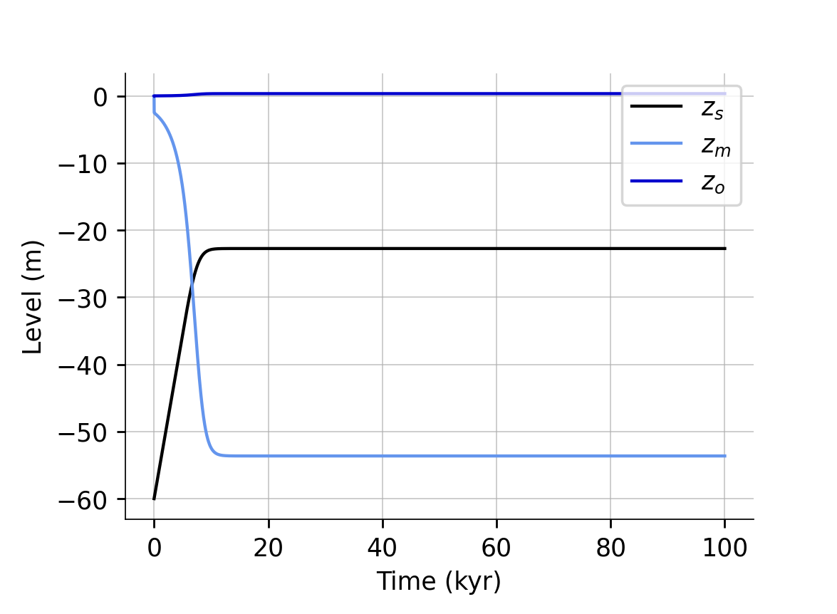
Figure 2 shows results for the reference parameter values. First, MSL rapidly drops several meters over about 25 years. This is an initial adjustment to the Mediterranean’s imbalanced water budget which starts the flow of water over the sill. After about 10 kyr, the model comes to rest with the Mediterranean level at roughly -54 m and the sill level at about -23 m. Uplift at the sill is exactly matched by erosion and the Mediterranean water budget is balanced. No oscillation is produced with the reference parameter values.
Next, I integrate the model for wide ranges of six key parameters. The “tested range” column of Table 2 shows the minimum and maximum value tested for each parameter. A set of twenty values spanning each range was generated. The values are uniformly spaced for all parameters except , where they are logarithmically spaced. Each of the ranges is roughly centered on the reference value except because the uplift rate is thought to be lower than the reference value of 4.9 mm/yr used in the original model (Duggen et al. 2003; Gerya et al. 2004; Andrews & Billen 2009; Duretz et al. 2011; Coulson et al. 2019). For all possible combinations of these parameter ranges—a total of 206 or 64 million combinations—the model was integrated and checked for oscillation using the steps described next.
To determine whether a set of parameters produces oscillations, the model is integrated in 25 kyr intervals for a maximum duration of 100 Myr, beginning with the initial conditions m and m. After each 25 kyr integration interval, the state of the system is checked. If the sill is above the ocean (), erosion and flow have ceased and the Mediterranean is disconnected. In this case, the sill will rise indefinitely, the system is not oscillating, and integration stops. Similarly, if the system appears to reach a stable fixed point, where and are no longer changing ( and ), then the system is not oscillating and integration stops. If integration proceeds for the entire 100 Myr limit without Mediterranean disconnection or arrival at a fixed point, the solution is assumed to be oscillating.
To determine if the system is at (or very near) a stable fixed point, a two-stage check is performed.
- 1.
The magnitudes of and are both less than 1 micrometer per year (3.169 m/s)
- 2.
A fixed point exists near the current model state and both system variables are within 0.01 % of the fixed point’s coordinates.
If the first check is satisfied, the second check is performed. If the second check is also satisfied, the model is assumed to be stationary and integration stops. Fixed points are located using multivariate Newton’s method and a finite difference approximation of the system’s Jacobian. Performing this check in two stages prevents the initiation of Newton’s method when the solution is not near a fixed point. This stringent, two-stage test is designed to prevent any oscillatory solutions from being erroneously identified as stable ones.
Table 3 summarizes the outcomes of all parameter combinations. Most solutions arrive at a stable fixed point. Only 0.2 % of the solutions oscillate. Figure 3 shows the distribution of oscillatory solutions for each parameter range, with a dashed red line at each parameter’s reference value. For all parameters, oscillatory solutions are much more likely with higher values. No oscillations occur in the lower end of the ranges for , , , and . Oscillation is particularly dependent on higher values of and , where there is a complete lack of oscillatory solutions at and below the reference values.
Figure 4 shows ten integrations with parameter combinations chosen randomly from the oscillatory solutions. Only the Mediterranean level (blue) and sill level (black) are shown, for clarity. The amplitudes of the oscillations here are all significantly less than in prior modeling, where MSL consistently reached -400 m and lower. The frequencies are also much higher. The oscillatory solutions tend to have many more than the roughly 16 cycles shown in previous work over 100 kyr. With higher values of and , the system increasingly resembles a relaxation oscillator. The third simulation from the bottom of Figure 4 is a good example. Hydrological energy builds up as slowly drops, culminating in extremely rapid erosion of the sill and reflooding of the Mediterranean. Once the critical shear stress is exceeded, erosion grows exponentially. For higher values of and , this transition from no erosion to very high erosion occurs extremely rapidly.
REVISITING CHANNEL SLOPE
An important component of the model is the slope of the water surface in the channel connecting the Atlantic and Mediterranean. This slope controls erosion on the sill through equations (4) and (5). It also controls discharge into the Mediterranean through equations (9) and (10). In this section, I analyze the choice of equation (6) for the channel slope and its consequences for model oscillation.
The Slope Equation
Garcia-Castellanos & Villaseñor 2011 use equation (6) to express the average slope between the Atlantic and Mediterranean. This is a simple and clear expression. However, to calculate this average slope, they choose a constant horizontal distance of 100 km. It is not clear why the horizontal distance between the Atlantic and the shore of the Mediterranean would be constant as MSL varies over hundreds of meters in the model.
As the Mediterranean level rises and falls, the horizontal distance between the sill and the sea would change. The change in this horizontal distance would be governed by the bathymetry of the Mediterranean near the sill. For example, if MSL drops 100 m and the average slope of the newly exposed terrain is 1 %, the horizontal length of the channel has increased 10 km. Figure 5 shows a schematic of this relationship between MSL, the channel length , and the average channel slope . More realistically, and would covary and the slope would be nearly constant for small changes in .
To calculate the true average slope along the channel, detailed bathymetry would be required. We do not know the exact bathymetry of the Mediterranean during the MSC, but we can consider modern data for intuition. Figure 6 shows modern bathymetry at the Strait of Gibraltar and into the western Mediterranean basin. If modern bathymetry is any guide, there is little reason to expect a constant channel length of 100 km as MSL varies over hundreds of meters. In fact, the average slope would probably decrease when MSL drops, not increase, because deeper parts of the strait and nearby basin are flatter.
Further, the nonuniform slope through the modern strait raises doubts about whether the average slope is most applicable when MSL varies hundreds of meters. Although the average slope is simple and convenient, the local slope near the sill may be different than the average slope when MSL drops significantly. We do not know the shape of the sill during the Messinian, but we can consider the modern configuration again as an example. If MSL dropped below the Camarinal Sill today, erosion on the sill would likely be controlled by the higher local slope, at least until erosion significantly modified the sill’s profile.
In this scenario, where erosion occurs primarily over steeper terrain near the sill, the slope could theoretically be computed over a fixed length and depend on the height of the sill as it rises and falls. This conception is illustrated in Figure 7. However, this representation would require an equation for the slope that depends on sill height, , and equation (6) does not depend on the sill height in any way. It depends only on and , with constant . Therefore, equation (6) does not represent an average local slope on the sill being slowly modified by uplift.
To summarize, if equation (6) is meant to represent the average slope between the Atlantic and Mediterranean sea levels, it should account for changing channel length instead of assuming is constant. There is no reason to expect Mediterranean sea level to rise and fall hundreds of meters without any lateral movement of the shoreline. If instead, equation (6) is meant to represent a more local slope near the sill as it is uplifted and eroded, it fails to capture this process because it does not depend on the sill height.
Implications for Oscillation
Whichever vision of the average slope (Figure 5 or 7) is preferred, equation (6) is not sufficiently representative. This is an important concern, as the choice of equation (6) is critical to the model’s capacity to oscillate. For oscillation to occur, there must be feedback that increases erosion when the Mediterranean level drops. In this model, a decrease in causes an increase in the slope , strengthening erosion and opening the channel to flood the Mediterranean and raise again. The dependence of on creates the necessary feedback. Without this dependence, the feedback from to is broken.
Crucially, it is the proposed form of equation (6), with average slope calculated using fixed , that introduces the dependence of on . Because changes in are much smaller than changes in ( %), the slope in equation (6) is approximately a linear function of . When drops, increases proportionally. However, as discussed above, the mean slope would probably be constant or decrease, not increase, if the change in and basin bathymetry are accounted for. Alternatively, if the local slope on the sill is more important than the mean slope, would not respond to the value of at all. In both cases, a more realistic representation of the slope is likely to render limit cycles impossible in this simple model because it would remove the proportional relationship between and . When MSL drops, there would not be increased erosion on the sill to deepen the channel, refill the Mediterranean, and generate limit cycles.
DISCUSSION & CONCLUSION
In the Model Setup section, I introduced a simplified and consolidated version of a prior model used to explain the evaporite cycles of the first stage of the MSC (Garcia-Castellanos & Villaseñor 2011). The model is comprised of two ODEs with two supporting expressions and no need for additional data. It can be solved by any standard ODE integration method. In the Simulations section, I integrated the model for the same parameters used in the main results of prior work (Garcia-Castellanos & Villaseñor 2011), finding a stable solution without oscillation (Figure 2). Then, using wide ranges of values for six key parameters, I checked all possible combinations of these values for oscillatory model solutions. Of the 64 million unique combinations checked, only 0.2 % exhibit oscillation and these combinations are strongly skewed toward higher parameter values in each case. The simulations that do produce oscillations generally have amplitudes and frequencies quite different than those in prior work. It appears that limit cycles in the proposed model are not a robust result.
The discrepancy between the results here and the results of prior work is not readily explained. The only substantive change to the model equations used here is the treatment of the Mediterranean as a single basin. The prior model divides the eastern and western basins when falls below -430 m. There is, however, no obvious reason that this division would be necessary for oscillation. Similarly, although the Mediterranean area and ocean level are implemented with an explicit expression here instead of interpolation, this should not change the behavior of the model. Finally, it is always possible that different numerical implementations or programming mistakes may have influenced the results. Prior work implements a customized “explicit finite-difference, time-iterative technique” to integrate the model, although this appears to simply be Euler’s method (Garcia-Castellanos 2011). For the present study, considerable effort was directed toward preventing numerical or programming problems. The simplified model was implemented in different programming languages and with distinct integration algorithms but yielded identical results for all tested parameter combinations. Additionally, both implementations rely on validated, publicly available integration codes (Virtanen et al. 2020; Baum 2021a).
In the Revisiting Channel Slope section, I explained how equation (6) is not physically representative of an average slope between the Atlantic and Mediterranean. To calculate the average channel slope, it assumes the horizontal position of the Mediterranean shoreline is fixed, even as the Mediterranean sea level varies tens or hundreds of meters. It is also not representative of the scenario where erosion is controlled by the local slope on the sill as the sill is uplifted and eroded. This is simply because equation (6) is completely independent of the sill height . In either case, the channel slope should not significantly increase when decreases. The rate of erosion on the sill need not depend on Mediterranean sea level because the shore is downstream of the erosion process. This is a critical problem because the unrepresentative dependence of on introduced by equation (6) is required to produce oscillations in this model.
Future work could develop an improved expression for the model slope. However, this will likely be a nontrivial task. A correct formulation must handle the condition where and . This is when the ocean is connected to the Mediterranean, as it is today with an open strait. When this happens, erosion and flow on the sill are poorly represented by idealized equations for stream dynamics. Proper treatment may have to dynamically account for periods when the sill is more like the ocean floor, instead of the bed of a stream. Further, as Coulson et al. 2019 show, future work must also account for the gravitational and isostatic effects of the changing water loads.
In conclusion, the proposed model only rarely exhibits limit cycles, and limit cycles require parameter values considerably higher than those originally reported. However, the proposed model includes an unphysical representation of the channel slope. This is important because the proposed form of the channel slope is crucial to the model’s capacity to oscillate. Properly treating the channel slope would make limit cycles unlikely for any parameter combinations and prior results should be reconsidered (Garcia-Castellanos & Villaseñor 2011; Coulson et al. 2019). A model with physically realistic slope equations might reveal whether sea-level limit cycles played a role in the mysterious first stage of the MSC, or if it must be explained by other mechanisms.
Acknowledgments
I would like to thank two anonymous reviewers for very helpful feedback regarding the full scope and context of the MSC. I would also like to thank Jerry Mitrovica, Daniel Garcia-Castellanos, and Robin Wordsworth for their open, supportive, and objective discussions about this work. The primary computations in this paper were run on the FASRC Cannon cluster supported by the FAS Division of Science Research Computing Group at Harvard University. Integration methods from libode (Baum 2021a) and SciPy (Virtanen et al. 2020) were used. Plots were created using the Matplotlib library (Hunter 2007). All code used for the analysis and plots in this paper is permanently archived in Zenodo (Baum 2021) and available with documentation at github.com/markmbaum/messinian-salinity-crisis.
References
- Andrews & Billen (2009) Erin. Andrews and Magali. Billen “Rheologic controls on the dynamics of slab detachment” In Tectonophysics 464.1-4, 2009 DOI: 10.1016/j.tecto.2007.09.004
- Baum (2021) Mark Baum “markmbaum/messinian-salinity-crisis v1” Zenodo, 2021 DOI: 10.5281/zenodo.4571688
- Baum (2021a) Mark Baum “wordsworthgroup/libode v1.0.3” Zenodo, 2021 DOI: 10.5281/zenodo.4429314
- CIESM (2008) CIESM “The Messinian Salinity Crisis from Mega-deposits to Microbiology” In CIESM Workshop Monographs 33 CIESM, 16 bd de Suisse, MC-98000, Monaco., 2008, pp. 1–168
- Coulson et al. (2019) Sophie Coulson, Tamara Pico, Jacqueline Austermann, Evelyn Powell, Robert Moucha and Jerry. Mitrovica “The role of isostatic adjustment and gravitational effects on the dynamics of the Messinian salinity crisis” In Earth and Planetary Science Letters 525, 2019 DOI: 10.1016/j.epsl.2019.115760
- De Lange & Krijgsman (2010) Gert. De Lange and Wout Krijgsman “Messinian salinity crisis: A novel unifying shallow gypsum/deep dolomite formation mechanism” In Marine Geology 275.1-4, 2010 DOI: 10.1016/j.margeo.2010.05.003
- Duggen et al. (2003) Svend Duggen, Kaj Hoernle and Jason Morgan “Deep roots of the Messinian salinity crisis”, 2003
- Duretz et al. (2011) Thibault Duretz, Taras. Gerya and Dave. May “Numerical modelling of spontaneous slab breakoff and subsequent topographic response” In Tectonophysics 502.1-2, 2011 DOI: 10.1016/j.tecto.2010.05.024
- EMODnet Bathymetry Consortium (2018) EMODnet Bathymetry Consortium “EMODnet Digital Bathymetry (DTM 2018)” EMODnet Bathymetry Consortium, 2018 DOI: 10.12770/18ff0d48-b203-4a65-94a9-5fd8b0ec35f6
- Garcia-Castellanos & Villaseñor (2011) D. Garcia-Castellanos and A. Villaseñor “Messinian salinity crisis regulated by competing tectonics and erosion at the Gibraltar arc” In Nature 480.7377, 2011 DOI: 10.1038/nature10651
- Garcia-Castellanos (2011) Daniel Garcia-Castellanos “asalted”, 2011 URL: https://github.com/danigeos/asalted
- Gargani & Rigollet (2007) Julien Gargani and Christophe Rigollet “Mediterranean Sea level variations during the Messinian salinity crisis” In Geophysical Research Letters 34.10, 2007 DOI: 10.1029/2007GL029885
- Gerya et al. (2004) Taras. Gerya, David. Yuen and Walter. Maresch “Thermomechanical modelling of slab detachment” In Earth and Planetary Science Letters 226.1-2, 2004 DOI: 10.1016/j.epsl.2004.07.022
- Hsü et al. (1973) K.. Hsü, W… Ryan and M.. Cita “Late Miocene Desiccation of the Mediterranean” In Nature 242.5395, 1973 DOI: 10.1038/242240a0
- Hunter (2007) J.. Hunter “Matplotlib: A 2D graphics environment” In Computing in Science & Engineering 9.3 IEEE COMPUTER SOC, 2007, pp. 90–95 DOI: 10.1109/MCSE.2007.55
- Just et al. (2011) Janna Just, Christian Hübscher, Christian Betzler, Thomas Lüdmann and Klaus Reicherter “Erosion of continental margins in the Western Mediterranean due to sea-level stagnancy during the Messinian Salinity Crisis” In Geo-Marine Letters 31.1, 2011 DOI: 10.1007/s00367-010-0213-z
- Krijgsman et al. (2001) W. Krijgsman, A.R. Fortuin, F.J. Hilgen and F.J. Sierro “Astrochronology for the Messinian Sorbas basin (SE Spain) and orbital (precessional) forcing for evaporite cyclicity” In Sedimentary Geology 140.1-2, 2001 DOI: 10.1016/S0037-0738(00)00171-8
- Krijgsman et al. (1999) W. Krijgsman, F.. Hilgen, I. Raffi, F.. Sierro and D.. Wilson “Chronology, causes and progression of the Messinian salinity crisis” In Nature 400.6745, 1999 DOI: 10.1038/23231
- Lugli et al. (2010) Stefano Lugli, Manzi Vinicio, Roveri Marco and Schreiber. Charlotte “The Primary Lower Gypsum in the Mediterranean: A new facies interpretation for the first stage of the Messinian salinity crisis” In Palaeogeography, Palaeoclimatology, Palaeoecology 297.1, 2010 DOI: 10.1016/j.palaeo.2010.07.017
- Manzi et al. (2013) Vinicio Manzi, Rocco Gennari, Frits Hilgen, Wout Krijgsman, Stefano Lugli, Marco Roveri and Francisco. Sierro “Age refinement of the Messinian salinity crisis onset in the Mediterranean” In Terra Nova 25.4, 2013 DOI: 10.1111/ter.12038
- Meijer & Krijgsman (2005) P Meijer and W Krijgsman “A quantitative analysis of the desiccation and re-filling of the Mediterranean during the Messinian Salinity Crisis” In Earth and Planetary Science Letters 240.2, 2005 DOI: 10.1016/j.epsl.2005.09.029
- NOAA (2010) NOAA “Volumes of the World’s Oceans from ETOPO1”, 2010 URL: https://www.ngdc.noaa.gov/mgg/global/etopo1_ocean_volumes.html
- NOAA (2012) NOAA “Hypsographic Curve of Earth’s Surface from ETOPO1”, 2012 URL: https://www.ngdc.noaa.gov/mgg/global/etopo1_surface_histogram.html
- Ohneiser et al. (2015) Christian Ohneiser, Fabio Florindo, Paolo Stocchi, Andrew. Roberts, Robert. DeConto and David Pollard “Antarctic glacio-eustatic contributions to late Miocene Mediterranean desiccation and reflooding” In Nature Communications 6.1, 2015 DOI: 10.1038/ncomms9765
- Rohling et al. (2008) E.J. Rohling, R. Schiebel and M. Siddall “Controls on Messinian Lower Evaporite cycles in the Mediterranean” In Earth and Planetary Science Letters 275.1-2, 2008 DOI: 10.1016/j.epsl.2008.08.022
- Roveri et al. (2014) Marco Roveri, Rachel Flecker, Wout Krijgsman, Johanna Lofi, Stefano Lugli, Vinicio Manzi, Francisco. Sierro, Adele Bertini, Angelo Camerlenghi, Gert De, Rob Govers, Frits. Hilgen, Christian Hübscher, Paul. Meijer and Marius Stoica “The Messinian Salinity Crisis: Past and future of a great challenge for marine sciences” In Marine Geology 352, 2014 DOI: 10.1016/j.margeo.2014.02.002
- Simon & Meijer (2017) Dirk Simon and Paul Meijer “Salinity stratification of the Mediterranean Sea during the Messinian crisis: A first model analysis” In Earth and Planetary Science Letters 479, 2017 DOI: 10.1016/j.epsl.2017.09.045
- Strogatz (1994) Steven. Strogatz “Nonlinear Dynamics And Chaos”, 1994
- Turowski et al. (2007) Jens. Turowski, Dimitri Lague and Niels Hovius “Cover effect in bedrock abrasion: A new derivation and its implications for the modeling of bedrock channel morphology” In Journal of Geophysical Research 112.F4, 2007 DOI: 10.1029/2006JF000697
- Verner (2010) J.. Verner “Numerically optimal Runge–Kutta pairs with interpolants” In Numerical Algorithms 53.2-3, 2010 DOI: 10.1007/s11075-009-9290-3
- Virtanen et al. (2020) Pauli Virtanen, Ralf Gommers, Travis. Oliphant, Matt Haberland, Tyler Reddy, David Cournapeau, Evgeni Burovski, Pearu Peterson, Warren Weckesser, Jonathan Bright, Stéfan. van der Walt, Matthew Brett, Joshua Wilson, K. Millman, Nikolay Mayorov, Andrew.. Nelson, Eric Jones, Robert Kern, Eric Larson, C Carey, İlhan Polat, Yu Feng, Eric. Moore, Jake VanderPlas, Denis Laxalde, Josef Perktold, Robert Cimrman, Ian Henriksen, E.. Quintero, Charles. Harris, Anne. Archibald, Antônio. Ribeiro, Fabian Pedregosa, Paul van Mulbregt and SciPy 1.0 Contributors “SciPy 1.0: Fundamental Algorithms for Scientific Computing in Python” In Nature Methods 17, 2020, pp. 261–272 DOI: 10.1038/s41592-019-0686-2
| Parameter | Fit Value |
|---|---|
| m2 | |
| 2754 m | |
| m2 | |
| 127.5 m |

| Parameter | Reference Value | Tested Range | Unit |
|---|---|---|---|
| 8 | 1 - 1 | m/yr Pa | |
| 50 | 25 - 100 | Pa | |
| 6 | 0.5 - 10 | - | |
| 4.9 | 0.49 - 4.9 | mm/yr | |
| 1.5 | 1 - 2 | - | |
| 100 | 50 - 150 | km | |
| 0.5 | s/m1/3 | ||
| 0.6 | m/yr | ||
| 1.2 | m/yr | ||
| 16500 | m3/s |
| Simulation Outcome | Percent |
|---|---|
| disconnection | 20.9 % |
| oscillation | 0.2 % |
| fixed point | 78.9 % |


