Comparison of compression vs shearing near jamming, for a simple model of athermal frictionless disks in suspension

In a recent work PeshkovTeitel2 we considered isotropic vs uniaxial compression, within a simple granular model of bidisperse non-Brownian spheres in suspension, as a means for numerically studying the effect of stress anisotropy on the jamming transition of frictionless particles. Isotropic compression at a finite rate results in configurations with an isotropic stress; there is a finite pressure but no shear stress. Uniaxial compression at a finite rate results in configurations with an anisotropic stress; there is both a finite pressure and a finite shear stress, similar to the case of sheared systems. Our analysis found that, in three dimensions, jamming via isotropic and uniaxial compression display the same universal critical behavior, despite the difference in stress symmetry.

In this work we consider more generally the differences between isotropically compressed, uniaxially compressed, pure sheared, and simple sheared configurations, when driven at a finite strain rate $\dot{\epsilon}$, as one approaches and goes above the jamming transition LiuNagel; OHern; OT1. For simplicity we consider the case of circular disks in two dimensions, using the same simple idealized model of a non-Brownian suspension as we used previously PeshkovTeitel2; PeshkovTeitel.

We compare the pressure $p$ and shear stress $\sigma$ arising from such deformations. Just below the jamming $\phi_{J}$, we find the pressure from isotropic and uniaxial compression to be equal within some range of $\phi$ depending on the initial sample preparation. The pressure from pure shearing and simple shearing are also roughly equal. However the pressure from pure/simple shearing is roughly an order of magnitude smaller than that from compression. The pressures in all four cases converge as $\phi$ increases above $\phi_{J}$. For the shear stress $\sigma$, we again find pure and simple shearing to give the same result. Below $\phi_{J}$, the shear stress for uniaxial compression becomes greater than for pure shear as $\phi$ decreases, while above $\phi_{J}$ it is reversed. From a comparison of the stress for these four deformations, we infer that the jamming $\phi_{J}$, and the critical exponents at jamming, are the same for isotropic and uniaxial compression. However we argue that the jamming $\phi_{J}^{*}$ for pure and simple shearing is slightly larger than the $\phi_{J}$ for compression. A critical scaling analysis for the case of pure shear, presented in Appendix B, gives a value for $\phi_{J}^{*}$ consistent with that previously found for simple shearing, while the critical exponents are consistent with those found for both simple shearing and for isotropic compression.

We also consider geometrical measures of the configurational contact network, particularly the average number of contacts per particle $Z$, and the fraction of contacts between the different types of particles in our bidisperse system. We find that, comparing the four types of deformation, these geometrical measures show small differences when one is below the jamming $\phi_{J}$, but that they become equal above $\phi_{J}$.

Finally, we compare the system anisotropy that results from uniaxial compression, pure shearing, and simple shearing. We show that the stress tensor anisotropy, measured by the macroscopic friction $\mu=\sigma/p$, behaves quite differently when comparing uniaxial compression with pure and simple shearing. For pure/simple shearing $\mu$ is monotonically decreasing as $\phi$ increases, while for uniaxial compression $\mu$ has a sharp minimum at $\phi_{J}$. The anisotropy of the contact network, as measured by the fabric tensor, shows similar behavior. We generalize these anisotropy measures to higher order orientational order parameters of both the force and contact network. Comparing uniaxial compression to pure shearing, we find that the main difference in anisotropy is the relative magnitude of the isotropic to nematic terms; higher order orientational moments behave similarly. In contrast, comparing simple shearing to pure shearing, we find that the isotropic and nematic terms are roughly equal, while the difference is in the higher order moments, which become equal as one approaches and goes above jamming, but become increasingly different as one goes below jamming.

The remainder of our paper is organized as follows. In Sec. II we present our model and numerical methods. In Sec. III we present our results for the the system stress, for uniaxial compression, isotropic compression, pure shearing, and simple shearing. In Sec. IV we present a discussion of the anisotropy of the configurational contact and force networks in these cases. In Sec. V we summarize our results. In Appendix A we provide a more complete discussion of the compression ensembles we use, discussing the dependence of the stress on the initial packing fraction $\phi_{\mathrm{init}}$ from which compression begins, and considering the $\phi_{\mathrm{init}}\to 0$ limit. In Appendix B we provide a more detailed discussion of pure shearing, including a critical scaling analysis.

Our model has been described in detail elsewhere PeshkovTeitel2; PeshkovTeitel. We simulate athermal ($T=0$), bidisperse, frictionless soft-core disks in two dimensions, with equal numbers of big and small disks with diameter ratios $d_{b}/d_{s}=1.4$ OHern. Particles, with centers of mass at positions $\mathbf{r}_{i}$, interact with a one-sided harmonic contact repulsion,

where $k_{e}$ is a stiffness constant, $r_{ij}=|\mathbf{r}_{i}-\mathbf{r}_{j}|$ and $d_{ij}=(d_{i}+d_{j})/2$. The elastic force acting on particle $i$ due to its contact with $j$ is then,

As a simplified model for particles in solution, we add a dissipative force due to the viscous drag on the particle with respect to the local velocity of the suspending host medium OT1; OT2; Durian,

where $k_{d}$ is a dissipative constant, $V_{i}$ is the area of particle $i$, and $\mathbf{v}_{\mathrm{host}}(\mathbf{r})$ is the velocity of the host medium at position $\mathbf{r}$. Particle motion is then determined from these forces using Newton’s equation. We take particle masses to be proportional to their area, $m_{i}\propto V_{i}$. Because our particles are circular and frictionless, we ignore particle rotations.

For the linear deformations we consider in this work, the background host velocity can be expressed in terms of the strain rate tensor $\dot{\bm{\epsilon}}$,

We will consider the particular cases of uniaxial compression (uni), isotropic compression (iso), pure shear (ps), and simple shear (ss), with respective strain rate tensors,

For uniaxial compression, we compress along the $\mathbf{\hat{x}}$ direction holding the $\mathbf{\hat{y}}$ direction fixed, while for pure shearing we compress along $\mathbf{\hat{x}}$ while expanding along $\mathbf{\hat{y}}$ at the same rate. Note, the factor of 1/2 in $\dot{\bm{\epsilon}}_{\mathrm{iso}}$ is so that the rate of area change is the same for $\dot{\bm{\epsilon}}_{\mathrm{iso}}$ as for $\dot{\bm{\epsilon}}_{\mathrm{uni}}$. The factor of 1/2 in $\dot{\bm{\epsilon}}_{\mathrm{ps}}$ is so that we can then view uniaxial compression as a superposition of an isotropic compression plus a pure shear,

The simple shear can be viewed as a pure shear of rate $\dot{\epsilon}$ with compression along the $(1,-1)$ diagonal, combined with a rotation of the system with angular velocity $-(\dot{\epsilon}/2)\mathbf{\hat{z}}$ MHT.

Our particles are placed in a rectangular box with side lengths $\mathbf{L}=(L_{x},L_{y})$, centered at $\mathbf{r}=0$. For uniaxial compression, isotropic compression, and pure shear, as we make our elastic deformations, the box lengths vary according to

At each integration step, particles that would fall outside the system box are returned to the box using periodic boundary conditions PeshkovTeitel2. For simple shear, the box lenghts $(L_{x},L_{y})$ stay constant, and the box skews to a rhomboidal shape at a fixed rate, with Lees-Edwards boundary conditions being applied Lees. A sketch showing the geometry of our four linear deformations is shown in Fig. 1.

To carry out our numerical simulations, we recast our model in terms of three dimensionless parameters Vag. The first is the packing fraction $\phi$,

For both isotropic and uniaxial compression, $\phi$ increases with time as the system gets compressed. For the area-preserving pure and simple shear deformations, $\phi$ stays constant.

The second is the quality factor $Q$, which measures the strength of the dissipative force relative to the elastic force. If $\tau_{d}=m_{s}/k_{d}V_{s}$ and $\tau_{e}=\sqrt{m_{s}d_{s}^{2}/k_{e}}$ are the time scales associated with the dissipative and elastic forces Vag, we have,

As $Q$ decreases, inertial effects decrease. For $Q$ sufficiently small, behavior becomes independent of the particular value of $Q$ and one enters the overdamped limit corresponding to massless particles, $m_{s}\to 0$ Vag; VagbergOlssonTeitel. For our simulations we will use $Q=1$, which is sufficiently small to put us in this overdamped limit Vag.

In the $m_{s}\to 0$ overdamped limit both $\tau_{e}$ and $\tau_{d}\to 0$, however we can define a time scale that remains finite Vag,

Our third dimensionless parameter is then the dimensionless strain rate,

Henceforth we will take our unit of length to be $d_{s}=1$, and our unit of time to be $\tau_{0}=1$. Quoted values of $\dot{\epsilon}$ are therefore the same as $\dot{\epsilon}\tau_{0}$. We consider strain rates spanning the range $\dot{\epsilon}=10^{-8.5}$ to $10^{-4}$.

We use LAMMPS lammps to integrate the equations of motion, using a time step of $\Delta t/\tau_{0}=0.1$. Unless otherwise noted, we use $N=32768$ total particles. Our simulations for isotropic and uniaxial compression start with an initial configuration at low packing $\phi_{\mathrm{init}}=0.4$, constructed as follows. We place particles down one by one at random, but making sure that there are no particle overlaps; if an overlap occurs, we discard that particle and try again until all $N$ particles are placed in the box. For isotropic compression, we use a square box with $L_{x}=L_{y}$. For uniaxial compression we start at $\phi_{\mathrm{init}}$ with a rectangular box with $L_{y}<L_{x}$, such that the box becomes roughly square by the time we have compressed to the jamming $\phi_{J}$. For uniaxial and isotropic compression we average our results over 20 independent initial configurations. For our pure shear simulations we start at each $\phi$ with a configuration generated by our uniaxial compression protocol, using the same strain rate $\dot{\epsilon}$. For each $\dot{\epsilon}$ we shear to a total strain $\epsilon\sim 1$, dropping an initial $\epsilon\sim 0.2$ to reach the sheared steady-state, and then averaging over the remainder of the run (see Appendix B for details). We then average our results over 10 independent initial configurations, except for our slowest rates $\dot{\epsilon}\leq 10^{-7}$, where we use only a single initial configuration. For simple shear, we start at each $\phi$ with a totally random initial configuration, and energy relax the system without shearing for a time $10^{6}\Delta t$ to remove any initial unphysically large particle overlaps. We then shear the system, discarding the first $\epsilon\sim 1$ to reach the sheared steady-state, and then average over an additional strain of $\epsilon\sim 9$.

In this section we consider the stress generated in the system by the elastic deformations. We consider only the stress arising from the elastic forces, since this is the dominant term at low strain rates. The stress tensor can be expressed in terms of the force moments as OHern,

where $\langle\cdots\rangle$ denotes an average over our independent runs for compression, and an average over both strain and independent runs for shearing.

A dimensionless stress tensor can be defined as Vag,

The stress tensor may be written in the general form,

where the pressure $p$ is the isotropic part of the stress, given by the average of the eigenvalues of $\mathbf{p}$. The anisotropic part of the stress is given by the deviatoric stress $\sigma$, determined as half the difference of the eigenvalues,

We will refer to $\sigma$ as simply the shear stress.

For isotropic compression, symmetry gives that the stress tensor is isotropic, and so $\sigma=0$. For both uniaxial compression and pure shear, as in Fig. 1, symmetry requires the stress tensor be diagonal, so that $p_{xy}=0$ and the shear stress is $\sigma=\delta p$. For simple shearing, if our system were a uniform elastic continuum one would find $\delta p=0$ and so $\sigma=|p_{xy}|$. For our granular system we will find that, while $p_{xy}\gg\delta p$, $\delta p$ does not strictly vanish, and so $\sigma$ is given by the full expression of Eq. (22).

The pressure $p$ and shear stress $\sigma$ thus give two parameters characterizing the stress tensor. The third parameter needed to completely specify the stress tensor can be taken to be the orientation of the maximal stress axis, given by the eigenvector of the maximal eigenvalue of $\mathbf{p}$. We denote this by $\vartheta_{2}$, the angle of the maximal stress axis with respect to the $\mathbf{\hat{x}}$ direction. For our uniaxial compression and pure shear, where the maximal stress direction is along $\mathbf{\hat{x}}$ (see Fig. 1(a)(c)), symmetry requires $\vartheta_{2}=0$. For simple shear, since $p_{xy}\gg\delta p$, we have $\vartheta_{2}\approx-\pi/4$.

The area-preserving process of shearing at a finite rate defines a steady-state ensemble of configurations that becomes independent of the initial starting configuration, provided one shears sufficiently long. This has previously been observed for the case of simple shearing Vagberg.PRE.2011, and in Appendix B we confirm that it is also the case for pure shearing. Our results below for $p$ and $\sigma$ for both pure and simple shearing represent a time average over configurations, once this steady-state limit has been reached. The resulting values of $p$, $\sigma$ and $\vartheta_{2}$ are determined solely by the parameters $\phi$, $Q$ and $\dot{\epsilon}$.

For isotropic and uniaxial compression, however, the situation is not as simple. As one compresses, $\phi$ increases, and the ensemble of configurations one passes through can depend on the ensemble of initial configurations one starts the compression from. In our case, where we start from configurations of non-overlapping particles at an initial packing $\phi_{\mathrm{init}}$, our values of $p$ and $\sigma$ can depend not only on the parameters $\phi$, $Q$, and $\dot{\bm{\epsilon}}$, but also on the additional parameter $\phi_{\mathrm{init}}$. In Appendix A we consider this dependence of the stress on $\phi_{\mathrm{init}}$. We find that as $\phi_{\mathrm{init}}$ decreases, the stress for both isotropic and uniaxial compression approaches a well defined $\phi_{\mathrm{init}}\to 0$ limit. For $\phi_{\mathrm{init}}$ not too small, the resulting $p(\phi)$ and $\sigma(\phi)$ approach this limiting curve as $\phi$ reaches the dense limit, just below jamming. Since using very small $\phi_{\mathrm{init}}$ can be computationally expensive for the large $N=32768$ system size that we wish to use, to avoid finite size effects near jamming, here we use $\phi_{\mathrm{init}}=0.4$. We find that this $\phi_{\mathrm{init}}$ is sufficiently small that our results are roughly independent of $\phi_{\mathrm{init}}$ once $\phi\gtrsim 0.80$. Further details are presented in Appendix A.

In Fig. 2(a) we plot $p$ vs $\phi$, for several different strain rates $\dot{\epsilon}$, for our four types of deformation: uniaxial compression, isotropic compression, pure shear, and simple shear. The vertical dashed line in this figure shows the jamming transition for isotropic compression, $\phi_{J}=0.8415$, as we have determined previously PeshkovTeitel. As found before PeshkovTeitel2; OT1; PeshkovTeitel; OT2, we find here (not shown) that all four deformations have a linear rheology, $p\propto\dot{\epsilon}$, provided one is below and not too close to jamming. Above jamming, $p$ approaches a constant as $\dot{\epsilon}\to 0$. Comparing the four cases, for $\phi\lesssim\phi_{J}$, we see that $p_{\mathrm{iso}}$ is equal to $p_{\mathrm{uni}}$, $p_{\mathrm{ps}}$ is equal to $p_{\mathrm{ss}}$, but the shearing pressure is about a factor 10 smaller than that of compression. For $\phi\gtrsim\phi_{J}$, however, we see that the $p$ for all four cases are becoming equal as $\dot{\epsilon}\to 0$.

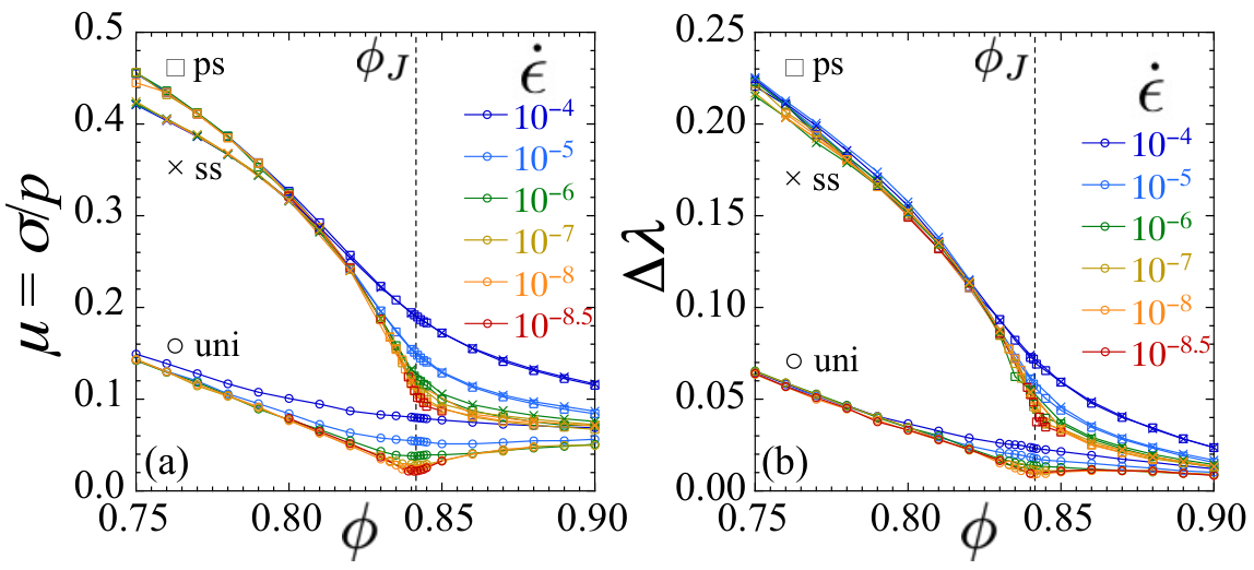
In Fig.  2(b) we similarly plot $\sigma$ vs $\phi$ at different $\dot{\epsilon}$, for uniaxial compression, pure shear, and simple shear ($\sigma_{\mathrm{iso}}=0$ by symmetry). As with the pressure $p$, the shear stress $\sigma\propto\dot{\epsilon}$ if one is not too close to jamming, while $\sigma$ approaches a constant as $\dot{\epsilon}\to 0$ above jamming. Here we see that that, as with the pressure, $\sigma_{\mathrm{ps}}$ is equal to $\sigma_{\mathrm{ss}}$. Comparing shearing to uniaxial compression, we see that $\sigma_{\mathrm{uni}}$ and $\sigma_{\mathrm{ps}}$ are generally of the same order of magnitude, but $\sigma_{\mathrm{ps}}<\sigma_{\mathrm{uni}}$ for $\phi\lesssim\phi_{J}$, while $\sigma_{\mathrm{ps}}>\sigma_{\mathrm{uni}}$ for $\phi\gtrsim\phi_{J}$. As $\dot{\epsilon}\to 0$, $\sigma_{\mathrm{ps}}/\sigma_{\mathrm{uni}}\to 1$ at $\phi\approx\phi_{J}$.

Next we consider some geometrical properties of our configurations. In Fig. 3(a) we plot the average number of contacts per particle $Z$ vs $\phi$ for our four types of deformation, at the two small strain rates $\dot{\epsilon}=10^{-7}$ and $10^{-8}$. As was observed before for isotropic compression PeshkovTeitel2 and simple shearing Heussinger1; OlssonRelax; Olsson3D, we find that, as $\dot{\epsilon}\to 0$, $Z$ stays finite and varies roughly linearly with $\phi$ for $\phi<\phi_{J}$, while at $\phi_{J}$ and above we see the square root singularity, $(Z-Z_{J})\sim(\phi-\phi_{J})^{1/2}$ associated with jamming PeshkovTeitel2; OHern; Wyart. Here our value of $Z_{J}$ at jamming is slightly below the isostatic value of $Z_{\mathrm{isostatic}}=2d=4$ since, for simplicity, we have not excluded rattler particles when computing $Z$ LiuNagel; OHern.

Our observation that $Z$ approaches a constant as $\dot{\epsilon}\to 0$ indicates that, at low strain rates, the system forms a well defined contact network at all packings, even below $\phi_{J}$. The extent of the particle overlaps at these contacts varies $\propto\dot{\epsilon}$, giving rise to the linear rheology in $p$ below $\phi_{J}$, however the geometry of the contact network remains the same. This is the hard-core limit. Similar to $p$, the contact numbers $Z$ for the four cases appear to become equal for $\phi\gtrsim\phi_{J}$, but differ below $\phi_{J}$, where $Z_{\mathrm{iso}}$ is roughly equal to $Z_{\mathrm{uni}}$, while $Z_{\mathrm{ps}}{\color[rgb]{0,0,0}=Z_{\mathrm{ss}}}$ is noticeably smaller than the other two.

In Fig. 3(b) we plot the fraction of the particle contacts that are between two small particles, two big particles, and between one small and one big particle vs $\phi$ for the strain rate $\dot{\epsilon}=10^{-7}$. Similar to $Z$ and $p$, we see that above $\phi_{J}$ these fractions become equal for all cases. Below $\phi_{J}$ we see that pure and simple shearing produce more small-small contacts and fewer big-big contacts than does isotropic or uniaxial compression. Our above results thus show that, in the jammed state above $\phi_{J}$, it is only the shear stress $\sigma$ that clearly distinguishes between compressive vs shearing deformations.

Next we consider whether all four cases jam at exactly the same critical packing fraction $\phi_{J}$. To investigate this we compute the stress ratios between the different cases. In Fig. 4(a) we compare uniaxial with isotropic compression, plotting $p_{\mathrm{uni}}/p_{\mathrm{iso}}$ vs $\phi$, for several different strain rates $\dot{\epsilon}$. We see no particular features as $\phi$ passes through $\phi_{J}$. Since, as $\dot{\epsilon}\to 0$, the bulk viscosity $\zeta\equiv p/\dot{\epsilon}\sim(\phi_{J}-\phi)^{-\beta}$ diverges at $\phi_{J}$ with the critical exponent $\beta$, the absence of any features in $p_{\mathrm{uni}}/p_{\mathrm{ps}}$ near $\phi_{J}$ strongly suggests that $p_{\mathrm{uni}}$ and $p_{\mathrm{iso}}$ jam at exactly the same $\phi_{J}$ and their $\zeta$ diverge with the same exponent $\beta$. This conclusion is in agreement with what we explicitly demonstrated for three dimensions in an earlier work PeshkovTeitel2.

In Fig. 4(b) we compare pure with simple shearing, plotting $p_{\mathrm{ss}}/p_{\mathrm{ps}}$ vs $\phi$. We similarly see no particular features as $\phi$ passes through $\phi_{J}$. The same behavior is found if we look at $\sigma_{\mathrm{ss}}/\sigma_{\mathrm{ps}}$. This suggests that pure and simple shearing jam at the same packing, with the same critical exponent $\beta$.

In Fig. 4(c) we compare compression with shearing, plotting $p_{\mathrm{uni}}/p_{\mathrm{ps}}$ vs $\phi$. Here we see a very different behavior. We find that $p_{\mathrm{uni}}/p_{\mathrm{ps}}$ develops a peak just below the isotropic compression-driven $\phi_{J}$; as $\dot{\epsilon}$ decreases, the height of this peak increases and the location of the peak moves closer to $\phi_{J}$. The same behavior is found for $\sigma_{\mathrm{uni}}/\sigma_{\mathrm{ps}}$ in  4(d).

Two possible explanations for such behavior are: (i) Shearing jams at a slightly higher $\phi_{J}^{*}$ than the $\phi_{J}$ for compression. In this case we would expect, in the limit $\dot{\epsilon}\to 0$, that $p_{\mathrm{uni}}/p_{\mathrm{ps}}$ diverges as $\phi\to\phi_{J}$ from below, stays infinite for $\phi_{J}<\phi<\phi_{J}^{*}$, and approaches a finite constant for all $\phi>\phi_{J}^{*}$. (ii) Shearing jams at the same $\phi_{J}$ as does compression, but with a smaller exponent $\beta^{*}<\beta$. In this case we would expect, in the limit $\dot{\epsilon}\to 0$, that $p_{\mathrm{uni}}/p_{\mathrm{ps}}$ diverges as $\phi\to\phi_{J}$ from below, but approaches a finite constant for all $\phi>\phi_{J}$. Our data is more consistent with the possibility (i), since we see that there remains a small interval above the compressive $\phi_{J}$ where the stress ratio continues to increase as $\dot{\epsilon}$ decreases. Prior work OT2; OT3 has demonstrated that for simple shearing our model jams at the packing $\phi_{J}^{*}=0.8435>\phi_{J}=0.8415$, and that the exponent $\beta$ is the same as found for compression PeshkovTeitel. In Appendix B we present a detailed critical scaling analysis of our pure shearing data that confirms that pure shearing indeed behaves the same as simple shearing, with the same $\phi_{J}^{*}>\phi_{J}$, and the same exponent $\beta$.

We have previously noted in Eq. (13) that, with regard to the strain rate tensor $\dot{\bm{\epsilon}}$, uniaxial compression can be regarded as a superposition of isotropic compression plus pure shearing. It is therefore natural to wonder whether a similar superposition holds for the resulting stresses in these flowing states, if one is in the region where the rheology is linear. Our results in Fig. 4, however, show that it does not. Were a superposition of stress to hold, we would expect $p_{\mathrm{uni}}=p_{\mathrm{iso}}+p_{\mathrm{ps}}$ and $\sigma_{\mathrm{uni}}=\sigma_{\mathrm{ps}}$ (since $\sigma_{\mathrm{iso}}=0$). Our results in Fig. 4, as well as our earlier results in Ref. PeshkovTeitel (see Fig. 1(b) of that work), show that for $\dot{\epsilon}\leq 10^{-7}$ we remain in the linear rheology region for $\phi$ up to at least $\sim 0.82$. However below $\phi=0.82$ we see from Figs. 4(a) and 4(d) that $p_{\mathrm{uni}}\approx p_{\mathrm{iso}}$ and $\sigma_{\mathrm{uni}}\approx 2.5\sigma_{\mathrm{ps}}$. In general, we see from Fig. 4(d) that $\sigma_{\mathrm{uni}}=\sigma_{\mathrm{ps}}$ only at an isolated point close to $\phi_{J}$. Thus there is no principle of superposition for stress in the flowing states below $\phi_{J}$.

In this section we consider the three elastic deformations that result in stress anisotropic systems, uniaxial compression, pure shearing, and simple shearing, and compare different measures of that anisotropy.

References

- (1) A. Peshkov and S. Teitel, Universality of stress-anisotropic and stress-isotropic jamming of frictionless spheres in three dimensions: Uniaxial versus isotropic compression, Phys. Rev. E 105, 024902 (2022).
- (2) A. J. Liu and S. R. Nagel, The jamming transition and the marginally jammed solid, Annu. Rev. Condens. Matter Phys. 1, 347 (2010).
- (3) C. S. O’Hern, L. E. Silbert, A. J. Liu, and S. R. Nagel, Jamming at zero temperature and zero applied stress: The epitome of disorder, Phys. Rev. E 68, 011306 (2003).
- (4) P. Olsson and S. Teitel, Critical scaling of shear viscosity at the jamming transition, Phys. Rev. Lett. 99, 178001 (2007).
- (5) A. Peshkov and S. Teitel, Critical scaling of compression-driven jamming of athermal frictionless spheres in suspension, Phys. Rev. E 103, L040901 (2021).
- (6) D. J. Durian, Foam mechanics at the bubble scale, Phys. Rev. Lett. 75, 4780 (1995) and Bubble-scale model of foam mechanics: Melting, nonlinear behavior, and avalanches, Phys. Rev. E 55, 1739 (1997).
- (7) P. Olsson and S. Teitel, Critical scaling of shearing rheology at the jamming transition of soft-core frictionless disks, Phys. Rev. E 83, 030302(R) (2011).
- (8) T. A. Marschall, D. Van Hoesen, and S. Teitel, Shear-driven flow of athermal, frictionless, spherocylinder suspensions in two dimensions: Particle rotations and orientational ordering, Phys. Rev. E 101, 032901 (2020).
- (9) D. J. Evans and G. P. Morriss, Statistical Mechanics of NonEquilibrium Liquids (Academic, London, 1990).
- (10) D. Vågberg, P. Olsson, and S. Teitel, Dissipation and rheology of sheared soft-core frictionless disks below jamming, Phys. Rev. Lett. 112, 208303 (2014).
- (11) D. Vågberg, P. Olsson, and S. Teitel, Critical scaling of Bagnold rheology at the jamming transition of frictionless two-dimensional disks, Phys. Rev. E 93, 052902 (2016).
- (12) See: https://lammps.sandia.gov/
- (13) D. Vågberg, P. Olsson, and S. Teitel, Glassiness, rigidity, and jamming of frictionless soft core disks, Phys. Rev. E 83, 031307 (2011).
- (14) C. Heussinger and J.-L. Barrat, Jamming transition as probed by quasistatic shear flow, Phys. Rev Lett. 102, 218303 (2009).
- (15) P. Olsson, Relaxation times and rheology in dense athermal suspensions, Phys. Rev. E 91, 062209 (2015).
- (16) P. Olsson, Dimensionality and viscosity exponent in shear-driven jamming, Phys. Rev. Lett. 122, 108003 (2019).
- (17) M. Wyart, L. E. Silbert, S. R. Nagel, and T. A. Witten, Effects of compression on the vibrational modes of marginally jammed solids, Phys. Rev. E 72, 051306 (2005).
- (18) P. Olsson and S. Teitel, Herschel-Bulkley shearing rheology near the athermal jamming transition, Phys. Rev. Lett. 109, 108001 (2012).
- (19) D. Vågberg, P. Olsson, and S. Teitel, Universality of jamming criticality in overdamped shear-driven frictionless disks, Phys. Rev. Lett. 113, 148002 (2014).
- (20) J. Zhang, T. Majmudar, A. Tordesillas, and R. Behringer, Statistical properties of a 2D granular material subjected to cyclic shear, Granul. Matter 12, 159 (2010).
- (21) A. Donev, J. Burton, F. H. Stillinger, and S. Torquato, Tetratic order in the phase behavior of a hard-rectangle system, Phys. Rev. B 73, 054109 (2006).
- (22) E. Azéma and F. Radjaï, Stress-strain behavior and geometrical properties of packings of elongated particles, Phys. Rev. E 81, 051304 (2010); Force chains and contact network topology in sheared packings of elongated particles, Phys. Rev. E 85, 031303 (2012); and Internal Structure of Inertial Granular Flows, Phys. Rev. Lett. 112, 078001 (2014).
- (23) T. S. Majmudar and R. P. Behringer, Contact force measurements and stress induced anisotropy in granular materials, Nature 435, 1079 (2005).
- (24) M. Ozawa, T. Kuroiwa, A. Ikeda, and K. Miyazaki, Jamming transition and inherent structures of hard spheres and disks, Phys. Rev. Lett. 109, 205701 (2012).
- (25) P. Charbonneau and P. K. Morse, Memory formation in jammed hard spheres, Phys. Rev. Lett. 126, 088001 (2021).
- (26) P. Olsson and S. Teitel, Athermal jamming versus thermalized glassiness in sheared frictionless particles, Phys. Rev. E 88, 010301(R) (2013).
- (27) T. Hatano, Growing length and time scales in a suspension of athermal particles, Phys. Rev. E 79, 050301(R) (2009).
- (28) M. Otsuki and H. Hayakawa, Critical behaviors of sheared frictionless granular materials near the jamming transition, Phys. Rev. E 80, 011308 (2009).
- (29) E. Lerner, G. Düring, and M. Wyart, A Unified framework for non-Brownian suspension flows and soft amorphous solids, Proc. Natl. Acd. Sci. U.S.A. 109, 4798 (2012).
- (30) E. DeGiuli, G. Düring, E. Lerner, and M. Wyart, Unified theory of inertial granular flows and non-Brownian suspensions, Phys. Rev. E 91, 062206 (2015).
- (31) T. Kawasaki, D. Coslovich, A. Ikeda, and L. Berthier, Diverging viscosity and soft granular rheology in non-Brownian suspensions, Phys. Rev. E 91, 012203 (2015).
- (32) B. Andreotti, J.-L. Barrat, and C. Heussinger, Shear flow of non-brownian suspensions close to jamming, Phys. Rev. Lett. 109, 105901 (2012).