The Milnor fiber conjecture of Neumann and Wahl,
and an overview of its proofThanks: ${\lx@sectionsign}$ Corresponding author

Maria Angelica Cueto, Patrick Popescu-Pampu^§ and Dmitry Stepanov To Norbert A’Campo, on the occasion of his 80^th birthday.

Date: 29 November 2022

Abstract.

Splice type surface singularities, introduced in 2002 by Neumann and Wahl, provide all examples known so far of integral homology spheres which appear as links of complex isolated complete intersections of dimension two. They are determined, up to a form of equisingularity, by decorated trees called splice diagrams. In 2005, Neumann and Wahl formulated their Milnor fiber conjecture, stating that any choice of an internal edge of a splice diagram determines a special kind of decomposition into pieces of the Milnor fibers of the associated singularities. These pieces are constructed from the Milnor fibers of the splice type singularities determined by the subdiagrams on both sides of the chosen edge. In this paper we give an overview of this conjecture and a detailed outline of its proof, based on techniques from tropical geometry and log geometry in the sense of Fontaine and Illusie. The crucial log geometric ingredient is the operation of rounding of a complex logarithmic space introduced in 1999 by Kato and Nakayama. It is a functorial generalization of the operation of real oriented blowup. The use of the latter to study Milnor fibrations was pioneered by A’Campo in 1975.

Key words and phrases:

Complete intersection singularities, integral homology spheres, Kato-Nakayama spaces, local tropicalization, log geometry, Milnor fibers, Newton non-degeneracy, real oriented blowups, rounding, Seifert fibrations, surface singularities, splice type singularities, toric geometry, toroidal varieties, tropical geometry

2020 Mathematics Subject Classification

Primary: 14B05, 14T90, 32S05; Secondary: 14M25, 57M15

1. Introduction

Let $(X,o)$ be an irreducible germ of a complex analytic surface with isolated singularity at $o$ , meaning that there exists a representative of it which is smooth outside $o$ , and also possibly at $o$ . We will say simply that $(X,o)$ is an isolated surface singularity. Denote by $\partial(X,o)$ its link, obtained by intersecting a representative $X$ embedded in $\mathbb{C}^{n}$ with a Milnor sphere, that is, a sphere centered at $o$ of radius $r_{0}>0$ , such that any sphere centered at $o$ of smaller radius is transversal to $X$ . The link $\partial(X,o)$ is a closed connected three-manifold, canonically oriented as the boundary of $(X\setminus\{o\})\cap\mathbb{B}(o,r_{0})$ , where $\mathbb{B}(o,r_{0})$ denotes the ball of radius $r_{0}$ .

The classical works [80], [52], [20] of Du Val, Mumford and Grauert show that oriented three-manifolds appearing as links of isolated surface singularities are exactly the graph manifolds which may be described by a negative definite and connected plumbing graph. Such oriented three-manifolds have canonical fillings (that is, compact oriented four-manifolds having them as boundaries), given by the minimal good resolutions of $(X,o)$ . Indeed, by work of Neumann [56, Theorem 2], the oriented topological type of the link determines the oriented topological type of the minimal good resolution.

Whenever $(X,o)$ is a complete intersection singularity, the link $\partial(X,o)$ admits another privileged filling, namely, the Milnor fiber of any smoothing $f:(Y,o)\to(\mathbb{C},0)$ of $(X,o)$ (i.e., $f$ is the germ of a holomorphic map with smooth generic fibers and special fiber identified with $(X,o)$ ), a notion originating in Milnor’s seminal book [50]. Indeed, by Tyurina’s [79, Theorem 8.1], the miniversal deformation of a complete intersection $(X,o)$ has an irreducible smooth base, therefore all the smoothings of $(X,o)$ have diffeomorphic Milnor fibers.

The following topological questions remain open:

1.

Which oriented three-dimensional graph manifolds occur as links of hypersurface or complete intersection isolated surface singularities?

2.

Which oriented four-dimensional manifolds occur as Milnor fibers of smoothings of hypersurface, complete intersection or arbitrary isolated surface singularities?

Most notably, very few conjectures have been proposed to address these questions. Among the most fruitful is the following one formulated by Neumann and Wahl in 1990 [59]:

Conjecture 1 (Casson Invariant).

If $(X,o)$ is a complete intersection isolated surface singularity and its link $\partial(X,o)$ is an integral homology sphere, then the Casson invariant of $\partial(X,o)$ is equal to one-eighth of the signature of the Milnor fiber of $(X,o)$ .

In [59], Neumann and Wahl confirmed several instances of this conjecture, including its validity for all weighted homogeneous singularities, all suspension hypersurface singularities and a particular family of singularities in $\mathbb{C}^{4}$ . What hindered further progress was the lack of other examples of complete intersections with integral homology sphere links.

Fifteen years later, Neumann and Wahl made a breakthrough in this direction, by introducing a wide class of examples, which they called splice type singularities [61]. This name is motivated by their construction. These singularities are defined by systems of equations whose structure is governed by special types of decorated trees, called splice diagrams, which were introduced by Siebenmann in [74] to encode graph manifolds which are integral homology spheres.

The term splicing was coined by Siebenmann to indicate a cut-and-paste operation introduced by Dehn in [13] to build new three-dimensional integral homology spheres from old ones. When splicing, solid tori are removed from two oriented integral homology spheres, and the resulting boundary 2-tori are then glued together by the unique isotopy class of diffeomorphisms which produces a new oriented integral homology sphere. Siebenmann proved that any integral homology sphere graph manifold can be obtained by iterating this operation, starting from Seifert fibered integral homology spheres and always removing tubular neighborhoods of fibers (which can be special or not). The starting Seifert-fibered manifolds are encoded by weighted star-shaped trees. Their edges correspond to the special fibers and to the fibers used during the splicing process, and the weights record the orders of holonomies around those fibers. The splicing is recorded by joining the corresponding edges of the two trees involved. The resulting weighted tree is Siebenmann’s splice diagram.

Neumann and Wahl’s splice type singularities are given by explicit systems of equations (see 2.34) associated to splice diagrams which satisfy supplementary constraints (see Definitions 2.25 and 2.29).

In [61, Section 6], Neumann and Wahl proposed an inductive approach for proving the Casson invariant conjecture for splice type singularities. The base case involved the so-called Brieskorn-Hamm-Pham complete intersections with integral homology sphere links which they had already established in [59]. The inductive step would be achieved by an explicit description of the topology of Milnor fibers in terms of splicing. To this end, they proposed the following conjecture (formulated precisely in 2.41):

Conjecture 2 (Milnor Fiber).

Let $(X,o)$ be a splice type singularity with an integral homology sphere link. Assume that its splice diagram $\Gamma$ is the result of splicing two other splice diagrams $\Gamma_{a}$ and $\Gamma_{b}$ . Then, the Milnor fiber of $(X,o)$ is obtained by a four-dimensional splicing operation from the Milnor fibers associated to $\Gamma_{a}$ and $\Gamma_{b}$ .

When restricted to the boundaries, Neumann and Wahl’s four-dimensional splicing operation becomes Dehn’s three-dimensional splicing. It resembles it in that it requires one to remove tubular neighborhoods of proper surfaces $G_{a}$ and $G_{b}$ embedded in the Milnor fibers $F_{a}$ and $F_{b}$ associated to $\Gamma_{a}$ and $\Gamma_{b}$ , but it differs from it in that one does not glue directly the resulting four-dimensional manifolds with corners. Instead, they are glued to parts of the boundary of a third manifold with corners, namely the cartesian product $G_{a}\times G_{b}$ .

The Casson invariant conjecture for splice type singularities with integral homology sphere links was proven by Némethi and Okuma [54] by rephrasing it as a statement about the geometric genus of the singularity $(X,o)$ . Their proof involved explicit computations with resolutions of $(X,o)$ , with no analysis of the Milnor fiber. As a result, the Milnor fiber conjecture remained open, only verified by Neumann and Wahl themselves for suspension hypersurface singularities (see [61, Section 8]) and by Lamberson [41] for iterated suspensions.

In this article, we present a step-by-step strategy for proving the Milnor fiber conjecture in full generality. Technical details will appear in forthcoming work by the three authors. Our proof combines tools from both tropical geometry and logarithmic geometry, in the sense of Fontaine and Illusie, and it is outlined in Section 7. Central to our arguments is the concept of rounding of a complex log structure in the sense of Kato and Nakayama, which can be viewed as a generalization of A’Campo’s real oriented blowup. Roundings allow us to find good representatives for Milnor fibrations without the need to work with tubular neighborhoods. In addition, rather than requiring good resolutions for our constructions, we broaden the setting and work with toric modifications involving toric varieties whose associated fans are not regular. This extended setting facilitates the transition from the tropical to the logarithmic category, since it allows us to work with natural fans subdividing the local tropicalizations of our germs, without the need to further refine them into regular fans.

Described very concisely, our proof involves the following stages, starting from a splice type singularity $(X,o)$ defined by a splice type system associated to a splice diagram $\Gamma$ :

(1)

We define a particular deformation of the splice type system, associated to a fixed internal edge $[a,b]$ of $\Gamma$ . We let $(Y,0)$ be the three-dimensional germ obtained as the total space of this deformation. We prove that the deformation is a smoothing $(Y,o)\to(\mathbb{D},0)$ of $(X,o)$ , where $\mathbb{D}$ denotes a compact two-dimensional disk with center $0$ .
(2)

Analogously, we define $a$ -side and $b$ -side deformations of $a$ -side and $b$ -side splice type singularities associated to the starting system, by performing special monomial changes of variables in the previous deformed system, that is, by taking pullbacks through special affine toric morphisms. We let $(Y_{a},o)$ and $(Y_{b},o)$ denote their total spaces.
(3)

We describe explicit fans subdividing the local tropicalizations of the deformations $(Y,o)$ , $(Y_{a},o)$ and $(Y_{b},o)$ , which are compatible with the local tropicalizations of the corresponding splice type singularities. As a preliminary step, we describe an explicit fan subdividing the local tropicalization of $(X,o)$ : topologically it is a cone over the corresponding splice diagram. This gives the first tropical interpretation of splice diagrams (see 2.36).
(4)

We consider toric birational morphisms defined by these three fans and the corresponding strict transforms of $(Y,o)$ , $(Y_{a},o)$ and $(Y_{b},o)$ , which we denote by $(\tilde{Y},o)$ , $(\tilde{Y}_{a},o)$ and $(\tilde{Y}_{b},o)$ , respectively. We show that the induced morphism from each strict transform to the corresponding germ is a modification, that is, a proper bimeromorphic morphism.
(5)

We consider the associated morphisms $(\tilde{Y},\mathcal{D})\to(\mathbb{D},0)$ , $(\tilde{Y}_{a},\mathcal{D}_{a})\to(\mathbb{D},0)$ , $(\tilde{Y}_{b},\mathcal{D}_{b})\to(\mathbb{D},0)$ , where $\mathcal{D}$ , $\mathcal{D}_{a}$ and $\mathcal{D}_{b}$ are the preimages of $0$ under the previous modifications. This allows us to apply a local triviality theorem of Nakayama and Ogus to the roundings of the associated logarithmic morphisms, yielding representatives of the Milnor fibrations of $(Y,o)\to(\mathbb{D},0)$ , $(Y_{a},o)\to(\mathbb{D},0)$ and $(Y_{b},o)\to(\mathbb{D},0)$ canonically associated to the previous modifications.
(6)

We show that the toric morphisms used to define the $a$ -side and $b$ -side deformations induce embeddings of suitable log enriched exceptional divisors of $\tilde{Y}_{a}\to Y_{a}$ and $\tilde{Y}_{b}\to Y_{b}$ into a similar enrichment of the exceptional divisor of $\tilde{Y}\to Y$ . This implies analogous results for their roundings.
(7)

These facts, combined with the knowledge that one of the components of the exceptional divisor of $\tilde{Y}\to Y$ is a cartesian product of two curves, establish the conjecture.

As a direct consequence of the proposed proof, we uncover an unknown property of splice type singularities (see Theorem 2.42):

Theorem.

The diffeomorphism type of the Milnor fiber of a splice type singularity with integral homology sphere link depends solely on the underlying splice diagram.

The combined use of tropical and logarithmic geometry techniques to study the topology of Milnor fibers is rather new. Since the inception of the research discussed in this paper and conference talks given by the second author on this subject, several articles applying logarithmic geometry to the study of problems about Milnor fibrations of singularities have appeared, including works of Cauwbergs [11], Bultot and Nicaise [9], Campesato, Fichou and Parusiński [10], and Fernández de Bobadilla and Pelka [16]. By presenting an overview of our techniques, we hope that this mainly expository article will help researchers apply similar ideas to address other questions involving the topological structure of Milnor fibers of smoothings of singularities.

The rest of the paper is organized as follows. In Section 2 we introduce background results leading to Neumann and Wahl’s notion of splice type singularities. Subsection 2.1 surveys their genesis by reviewing a presentation of the structure of Seifert fibered integral homology spheres and the way they appear as links of isolated complete intersections of Brieskorn-Pham hypersurface singularities. Subsection 2.2 provides detailed explanations on the three-dimensional splicing operation and splice type integral homology spheres. Subsection 2.3 reviews the construction of splice type singularities. Finally, Subsection 2.4 presents Neumann and Wahl’s four-dimensional splicing operation and the precise formulation of their Milnor fiber conjecture.

In Section 3 we discuss the main ideas of the proof of this conjecture. Subsection 3.1 shows that A’Campo’s operation of real oriented blowup yields canonical representatives of the Milnor fibration over the circle of a smoothing, provided we are given an embedded resolution of the smoothing. In our context we do not work with embedded resolutions, but with more general morphisms which we call quasi-toroidalizations. In Subsection 3.2 we present a general theorem of Nakayama and Ogus, stating the local triviality of a continuous map obtained by rounding in the sense of Kato and Nakayama of suitable logarithmic morphisms in the sense of Fontaine and Illusie. Finally, Subsection 3.3 shows how to build the aforementioned quasi-toroidalizations through explicit fan structures on the local tropicalizations of suitable deformations of splice type systems, combined with the Newton non-degeneracy property of these deformations.

Section 4presents detailed accounts of the logarithmic tools used to prove the Milnor fiber conjecture. In Subsection 4.1 we introduce the notions of boundary-transversality, of quasi-toroidal subboundary and of quasi-toroidalization of a smoothing. In Subsection 4.2 we lead the reader to the notion of log structure through a reformulation in a coordinate-independent way of the classical passage to polar coordinates. In Subsection 4.3 we explain basic facts about the category of morphisms of complex log spaces in the sense of Fontaine and Illusie. In Subsection 4.4 we list various kinds of monoids needed in the sequel, as well as the associated log structures, defined in terms of charts. In Subsection 4.5 we define Kato and Nakayama’s rounding operation on complex log spaces and we explain some of its basic properties. In Subsection 4.6 we revisit Nakayama and Ogus’ local triviality theorem and apply it in the context of quasi-toroidalizations of smoothings.

In Section 5 we introduce the tropical ingredients of our proof: the notion of local tropicalization of an analytic germ contained in $(\mathbb{C}^{n},0)$ and the notion of Newton non-degeneracy.

Section 6presents the explicit deformations of splice type systems appearing in Stage 2 above.

The paper concludes with Section 7, in which we give a detailed proof outline in $28$ steps of the six stages discussed earlier to establish the Minor fiber conjecture.

2. Splicing, splice type singularities and the Milnor fiber conjecture

The operation of splicing and the construction of splice type singularities are central components of the Milnor fiber conjecture. In this section, we review Seifert’s classification of Seifert fibered integral homology spheres, henceforth denoted by $\mathbb{Z}\!\operatorname{HS}$ ’s (see 2.9), Neumann’s realization of those $\mathbb{Z}\!\operatorname{HS}$ ’s as links of isolated complete intersections of Pham-Brieskorn-Hamm type (see 2.13) and the cut-and-paste operation of splicing of $\mathbb{Z}\!\operatorname{HS}$ ’s along knots (see 2.20). In addition, we recall the genesis of splice diagrams (see 2.22) as graphs introduced by Siebenmann to encode $\mathbb{Z}\!\operatorname{HS}$ ’s which are graph manifolds (see 2.23), and Eisenbud and Neumann’s characterization of splice diagrams encoding all singularity links which are $\mathbb{Z}\!\operatorname{HS}$ ’s (see Theorem 2.26). We describe how these results motivated Neumann and Wahl to define splice type systems and splice type singularities associated to splice diagrams which satisfy the so-called determinant and semigroup conditions (see Subsection 2.3). The section concludes with a discussion of Neumann and Wahl’s four-dimensional splicing operation (see 2.39) and with the statement of their Milnor fiber conjecture (see 2.41).

2.1. Seifert fibered integral homology spheres

We start this subsection by explaining the notions of integral homology sphere (or $\mathbb{Z}\!\operatorname{HS}$ , see 2.1), of meridian and longitude of a knot in a $\mathbb{Z}\!\operatorname{HS}$ (see 2.5) and of Seifert fibration (see 2.6). In addition, we discuss various results that predate the notion of splice type singularity, from the appearance of Poincaré’s homology sphere as the link of the $E_{8}$ surface singularity (see Subsection 2.1) to Seifert’s classification of Seifert fibered links of singularities which are moreover integral homology spheres (see 2.9).

In the sequel, we denote by $\boxed{\partial_{top}W}$ the boundary of a smooth or topological manifold with boundary. In contrast, we use $\boxed{\partial W}$ to denote the algebro-geometric boundary of a toroidal variety $(W,\partial W)$ (see 3.1). If $V\hookrightarrow W$ is a properly embedded submanifold with boundary of a manifold with boundary, we use $\boxed{N_{W}(V)}$ to denote a topologically closed tubular neighborhood of $V$ in $W$ . Note that $N_{W}(V)$ has the structure of a disk bundle over $V$ , whose fibers have dimension equal to the codimension of $V$ in $W$ , which we denote by $\boxed{\operatorname{codim}_{W}(V)}$ . Its intersection with $\partial_{top}W$ is a tubular neighborhood of the boundary $\partial_{top}V$ inside $\partial_{top}W$ .

The next class of three-dimensional manifolds is central to this paper:

2.1.

An integral homology sphere, briefly written $\boxed{\mathbb{Z}\!\operatorname{HS}}$ , is a closed smooth three-manifold which has the total integral homology group of a three-dimensional sphere. A $\mathbb{Z}\!\operatorname{HS}$ is called trivial if, and only if, it is homeomorphic to the unit three-dimensional sphere $\mathbb{S}^{3}$ .

2.2.

Important properties follow from the $\mathbb{Z}\!\operatorname{HS}$ condition. Indeed, if $M$ is a $\mathbb{Z}\!\operatorname{HS}$ , then $H_{0}(M,\mathbb{Z})\simeq\mathbb{Z}$ . Thus, $M$ must be connected. In addition, as $H_{3}(M,\mathbb{Z})\simeq\mathbb{Z}$ , we see that $M$ is also orientable.

2.3.

Fixing an orientation on a closed orientable three-manifold $M$ determines a well-defined Poincaré duality isomorphism $H_{2}(M,\mathbb{Z})\simeq H^{1}(M,\mathbb{Z})$ . Since $H^{1}(M,\mathbb{Z})$ $\simeq\Hom(H_{1}(M,\mathbb{Z}),\mathbb{Z})$ , by the universal coefficients theorem, we conclude that $M$ is a $\mathbb{Z}\!\operatorname{HS}$ if, and only if, it is a connected and orientable three-manifold with $H_{1}(M,\mathbb{Z})=0$ .

Throughout, we assume that all integral homology spheres are oriented, i.e., they are endowed with fixed orientations. Such manifolds $M$ admit a well-defined notion of linking number $\boxed{lk(K_{1},K_{2})}$ between any two disjoint oriented knots $K_{1},K_{2}$ on them: it is the intersection number between $K_{1}$ and an oriented surface $S_{2}\hookrightarrow M$ with boundary $K_{2}$ . The fact that such a surface exists and that this intersection number is independent of the choice of $S_{2}$ is a direct consequence of the vanishing of $H_{1}(M,\mathbb{Z})$ . The linking number is symmetric in its two arguments, a property which we will frequently exploit.

Given any integral homology sphere, the boundary of a tubular neighborhood of a knot in it is canonically trivialized, up to isotopy, as the next result shows. For more details, we refer to [15, page 21] and [74, §6].

2.4.

Let $M$ be an oriented $\mathbb{Z}\!\operatorname{HS}$ and let $K$ be an oriented knot in $M$ . Let $N_{M}(K)$ be a tubular neighborhood of $K$ in $M$ . Then, there exist embedded oriented circles $\mu$ and $\lambda$ on $\partial_{top}N_{M}(K)$ , well-defined up to isotopy, such that $lk(\mu,K)=1$ , $lk(\lambda,K)=0$ and the homology classes of $\lambda$ and $K$ in $H_{1}(N_{M}(K),\mathbb{Z})$ coincide. Moreover, the classes of $\mu$ and $\lambda$ in $H_{1}(\partial_{top}N_{M}(K),\mathbb{Z})$ form a basis of this lattice.

The previous statement determines the notions of meridian and longitude of oriented knots in integral homology spheres, which we now recall:

2.5.

Let $M$ be an oriented $\mathbb{Z}\!\operatorname{HS}$ and let $K$ be an oriented knot in $M$ . The oriented curves $\mu$ and $\lambda$ characterized in 2.4 are called a meridian and a longitude of $K$ , respectively.

Replace the previous paragraph with the following one: Sometimes, any oriented simple closed curve on $\partial_{top}N_{M}(K)$ whose homology class gives a basis of $H_{1}(\partial_{top}N_{M}(K),\mathbb{Z})$ when completed by that of $\mu$ is called a longitude of $K$ (the curves characterized in 2.5 being then called topologist’s longitudes). As we will not consider these more general types of longitudes, we refrain from using this terminology.

Meridians and longitudes are essential to defining three-dimensional splicings, as seen in 2.19 and 2.20 below. They are denoted by $m_{i}$ and $\ell_{i}$ in Figure 1.

The first example of non-trivial $\mathbb{Z}\!\operatorname{HS}$ was given by Poincaré in his 1904 paper [69]: it is the famous Poincaré homology sphere. He defined it using a Heegaard diagram. Notably, it can also be defined as the link of the $\boxed{E_{8}}$ surface singularity, i.e., the germ at the origin of the complex affine surface in $\mathbb{C}^{3}_{x,y,z}$ defined by the equation

x^{2}+y^{3}+z^{5}=0.

It is not at all obvious that these two three-manifolds are homeomorphic. This was established only after the introduction of Seifert fibered three-manifolds by Seifert in his 1933 paper [72]. The crux of the proof is to show that both manifolds are Seifert fibered integral homology spheres and that their Seifert fibrations have the same numerical invariants (see Subsection 2.1). For further details on the first studies of the Poincaré homology sphere, we refer to Gordon’s work [19, Section 6]. For other characterizations, the reader may consult Kirby and Scharlemann’s paper [38], or Saint Gervais’ website [71].

Next, we review the notion of Seifert fibration on closed oriented three-manifolds. For further details, the reader may consult Orlik’s book [65] or Neumann and Raymond’s paper [58].

2.6.

A Seifert fibration on a closed oriented three-manifold is an orientable foliation by circles. Its base is the space of leaves endowed with the quotient topology. Its fibre map is the quotient map. A manifold endowed with a Seifert fibration is called Seifert fibered.

2.7.

It can be shown that the base $S$ of a Seifert fibration on a closed oriented three-manifold $M$ is an orientable closed surface and that the fibre map $\psi\colon M\to S$ is a locally trivial circle bundle away from a finite set of points of $S$ . Those points correspond to the so-called special fibers of the Seifert fibration.

2.8.

Following Seifert’s original approach from [72, Section 1], Seifert fibrations are often defined as maps $\psi\colon M\to S$ which are locally trivial on $S$ away from the neighborhood of a finite set of points and which have prescribed models in the neighborhoods of the special fibers (see, for instance, [65, Section 5.2]). These models can be described using the holonomy of the foliation along a special fiber $C$ . Turning once around $C$ yields a diffeomorphism of a transversal slice, which is isomorphic to a finite-order rotation of a disk. Such a rotation may be encoded by a rational number $q/p\in(0,1)\cap\mathbb{Q}$ , with $p$ and $q$ coprime. The integer $p\geq 2$ is the order of the rotation, that is, the degree of the quotient map $\psi$ restricted to a transversal slice of $C$ . For this reason, we call it the degree of the point $\psi(C)\in S$ . It can also be interpreted as the number of times the leaves situated in the neighborhood of $C$ turn around $C$ .

The basic numerical invariants of a Seifert fibration are the pairs $(p,q)$ associated to its special fibers and the topological type of the base surface $S$ . These, combined with the rational Euler number of the fibration (see, e.g., [58, Section 1], [57, Section 1] or [29, Section I.3]), determine the fibration up to a homeomorphism of $M$ preserving the foliation and the orientation. For general Seifert fibrations, the Euler number is rational and it changes sign if the orientation on $M$ is reversed. When $\psi\colon M\to S$ is a locally trivial circle bundle, we have no special fibers and the rational Euler number of the fibration agrees with the usual Euler number of the bundle; thus, it is an integer.

Seifert fibrations of non-trivial integral homology spheres are well-understood, as the following theorem of Seifert confirms. For details, we refer the reader to works of Seifert [72, Theorem 12], Neumann and Raymond [58, Section 4] or Eisenbud and Neumann [15, Chapter II.7]):

2.9.

If $M$ is a non-trivial $\mathbb{Z}\!\operatorname{HS}$ that admits a Seifert fibration, then this fibration is unique up to isotopy. Furthermore, its base is a two-dimensional sphere and it has at least three special fibers, with pairwise coprime degrees. Conversely, given $n\geq 3$ and a sequence $(p_{1},\dots,p_{n})$ of pairwise coprime positive integers with $p_{i}\geq 2$ for all $i$ , there exists a unique Seifert fibered $\mathbb{Z}\!\operatorname{HS}$ up to homeomorphisms, whose base is a two-dimensional sphere and whose special fibers have degrees $p_{1},\dots,p_{n}$ . With either orientation, the Euler number of this fibration is non-zero.

The previous proposition allows to define integral homology spheres from sequences of pairwise coprime positive integers:

2.10.

Fix $n\geq 3$ and let $(p_{1},\dots,p_{n})$ be a sequence of pairwise coprime positive integers with $p_{i}\geq 2$ for all $i\in\{1,\ldots,n\}$ . The oriented three-dimensional manifold $\boxed{\Sigma(p_{1},\dots,p_{n})}$ is the unique oriented $\mathbb{Z}\!\operatorname{HS}$ which admits a Seifert fibration with a negative Euler number and whose sequence of degrees of special fibers is $(p_{1},\dots,p_{n})$ , up to permutation.

2.11.

Note that in both 2.9 and 2.10 we assume $p_{i}\geq 2$ for all $i\in\{1,\ldots,n\}$ . We can extend 2.10 to allow for $p_{i}\geq 1$ , by simply removing all terms of the sequence with value one, defining the corresponding Seifert fibered $3$ -manifold and identifying indices $i$ with $p_{i}=1$ with non-special fibers of the fibration. For instance, $\Sigma(1,1,3,8,35)=\Sigma(3,8,35)$ and the first two elements of the sequence $(1,1,3,8,35)$ witness two non-special fibers of $\Sigma(3,8,35)$ (see 2.16 below). Allowing some $p_{i}$ ’s to take value $1$ is important in the construction of integral homology spheres from splice diagrams (see 2.23 below).

2.11.

Consider the polynomial $f:=x^{2}+y^{3}+z^{5}$ defining the complex surface $X$ whose germ at the origin is the $E_{8}$ singularity. The polynomial $f$ is homogeneous relative to the weight vector $w:=(3\cdot 5,2\cdot 5,2\cdot 3)$ . Therefore, the surface $X$ is invariant under the following natural action of the group $(\mathbb{C}^{*}_{t},\cdot)$ on $\mathbb{C}^{3}_{x,y,z}$ :

(2.1)

t\cdot(x,y,z):=(t^{3\cdot 5}x,t^{2\cdot 5}y,t^{2\cdot 3}z).

Thus, it is invariant under the action of the circle $(\mathbb{S}^{1},\cdot)$ of $(\mathbb{C}^{*}_{t},\cdot)$ . Similarly, all Euclidean spheres $\mathbb{S}^{5}_{\varepsilon}$ centered at the origin of $\mathbb{C}^{3}_{x,y,z}$ (of radius $\varepsilon>0$ ) are invariant under this action of the circle. As a consequence, the intersections $X\cap\mathbb{S}^{5}_{\varepsilon}$ are also invariant. Note that the manifolds $X\setminus\{0\}$ and $\mathbb{S}^{5}_{\varepsilon}$ intersect transversally, as the orbits of the $(\mathbb{R}_{t}^{*},\cdot)$ -action on $X$ induced by the above $(\mathbb{C}_{t}^{*},\cdot)$ -action are transversal to the spheres $\mathbb{S}^{5}_{\varepsilon}$ . Therefore, these intersections are representatives of the link $\partial(X,0)$ of the singularity $(X,0)$ . In particular, this shows that there exists an action of $(\mathbb{S}^{1},\cdot)$ on this link with no fixed points. Its orbits determine a Seifert fibration on $\partial(X,0)$ .

A closer look at the action (2.1) confirms that the previous Seifert fibration has exactly three special fibers (the intersections with the planes of coordinates), with degrees $2,3$ and $5$ . Moreover, $\partial(X,0)$ is a $\mathbb{Z}\!\operatorname{HS}$ . This fact may be proved in several ways:

•

By seeing it as a ramified cover of $\mathbb{S}^{3}$ of degree $5$ , ramified over the trefoil knot, and using Seifert’s characterization [72, Addendum to Theorem 17, page 413 of the English version of Seifert and Threlfall’s book]) of such covers which are integral homology spheres.
•

By using Brieskorn’s criterion [7, Satz 1, page 6] (see also Dimca’s [14, Theorem 4.10, page 94]), described first in a letter of Milnor to Nash (see [8, page 47]), allowing to determine when the link of a Pham-Brieskorn hypersurface singularity of arbitrary dimension (see 2.14) is an integral homology sphere.
•

By computing the weighted dual graph of the minimal good resolution of $(X,0)$ , which is a tree of components of genus zero (it is the so-called $E_{8}$ -tree of Lie groups theory), and by proving that the associated intersection form is unimodular, which implies that the link is indeed an integral homology sphere (see [14, Proposition 3.4, page 52]). The weighted dual graph may be computed either using the Jung-Hirzebruch method, as explained by Laufer [42, pages 23–27] or using the $(\mathbb{C}_{t}^{*},\cdot)$ -action, as explained by Orlik and Wagreich in [66, Section 3] (see also [14, pages 64–67] and [51, Theorem 4.2]).
•

By using the facts that the intersections $Z(x|_{X}),Z(y|_{X}),Z(z|_{X})$ of $X$ with the three coordinate planes are irreducible germs of curves and that their strict transforms by the minimal good resolution $\pi:\tilde{X}\to X$ of $X$ intersect transversally the exceptional divisor $E$ at its components associated with the leaves of the dual tree. Then, Neumann and Wahl’s [62, Proposition 5.1] implies that the duals of those components (in the intersection lattice $H_{2}(E,\mathbb{Z})$ of $E$ endowed with its intersection form inside $\tilde{X}$ ) generate the discriminant group $H_{2}(E,\mathbb{Z})^{\vee}/H_{2}(E,\mathbb{Z})$ of $E$ , which identifies canonically to $H_{1}(\partial(X,0),\mathbb{Z})$ . The irreducibility and the transversality properties mentioned above imply that those duals are equal to the opposites of the exceptional parts of the total transforms of $Z(x|_{X}),Z(y|_{X}),Z(z|_{X})$ by $\pi$ . Thus they have integral coefficients, that is, they belong to $H_{2}(E,\mathbb{Z})$ . This implies that the discriminant group is trivial, therefore $H_{1}(\partial(X,0),\mathbb{Z})$ is also trivial.

2.9ensures now that $\partial(X,0)$ is the Seifert fibered integral homology sphere $\Sigma(2,3,5)$ .

Work of Neumann [55] characterizes the integral homology sphere $\Sigma(p_{1},\dots,p_{n})$ as a singularity link:

2.12.

Fix $n\geq 3$ and let $(p_{1},\dots,p_{n})$ be a sequence of pairwise coprime positive integers with $p_{k}\geq 2$ for all $k\in\{1,\ldots,n\}$ . Let $(c_{i,j})_{1\leq i\leq n-2,1\leq j\leq n}$ be a matrix of complex numbers all of whose maximal minors are non-zero. Then, the subspace of $\mathbb{C}^{n}$ defined by the system of equations:

(2.2)

\left\{\begin{array}[]{cccccc}c_{1,1}z_{1}^{p_{1}}&+&\cdots&+&c_{1,n}z_{n}^{p_{n}}&=0,\\ \vdots&\vdots&\vdots&\vdots&\vdots&\vdots\\ c_{n-2,1}z_{1}^{p_{1}}&+&\cdots&+&c_{n-2,n}z_{n}^{p_{n}}&=0,\end{array}\right.

is an irreducible surface with an isolated singularity at $0$ whose link, oriented as the boundary of a neighborhood of $0$ , is (orientation-preserving) homeomorphic to the integral homology sphere $\Sigma(p_{1},\dots,p_{n})$ .

The condition that all the maximal minors of the matrix of coefficients are non-zero is equivalent to the condition that the previous system defines an isolated complete intersection singularity at the origin of $\mathbb{C}^{n}$ . This is a direct consequence of the following more general result of Hamm (see [23, §5] and [25]):

2.13.

Fix $n\geq 3$ and let $(p_{1},\dots,p_{n})$ be a sequence of positive integers with $p_{i}\geq 2$ for all $i\in\{1,\ldots,n\}$ , and fix $k\in\{1,\dots,n-1\}$ . Consider a $k\times n$ -matrix $(c_{i,j})_{i,j}$ with complex entries. Then, the system of equations

(2.3)

\left\{\begin{array}[]{cccccc}c_{1,1}z_{1}^{p_{1}}&+&\cdots&+&c_{1,n}z_{n}^{p_{n}}&=0,\\ \vdots&\vdots&\vdots&\vdots&\vdots&\vdots\\ c_{k,1}z_{1}^{p_{1}}&+&\cdots&+&c_{k,n}z_{n}^{p_{n}}&=0,\end{array}\right.

defines an isolated complete intersection singularity at $0$ in $\mathbb{C}^{n}$ if, and only if, all maximal minors of the input matrix $(c_{i,j})_{i,j}$ are non-zero.

2.14.

Notice that each equation of (2.3) defines a so-called Pham-Brieskorn hypersurface singularity (see Brieskorn’s paper [8, pages 47–49] for an explanation of this terminology). For this reason, isolated complete intersection singularities (ICIS) defined by these systems are sometimes called Pham-Brieskorn-Hamm singularities.

2.15.

If a Pham-Brieskorn-Hamm singularity of complex dimension at least three has an integral homology sphere link (i.e., its link has the integral homology of a sphere of the same dimension), then this link is homeomorphic to a sphere. Indeed, as proved by Milnor [50, Theorem 5.2] for isolated singularities of hypersurfaces and extended by Hamm [24, Kor. 1.3] to ICIS, their links are simply connected. In turn, by a theorem of Smale [75], a simply connected integral homology sphere of dimension at least five is homeomorphic to a sphere. Brieskorn discovered in [7] (see also [8]) that for hypersurfaces, such links could be exotic spheres. Subsequent work by Hamm [25] extended the study of such exotic spheres to all Pham-Brieskorn-Hamm singularities.

2.16.

Notably, the link of a Pham-Brieskorn-Hamm surface singularity $(X,0)$ defined by the system (2.2) is always Seifert-fibered, even when it is not an integral homology sphere. This fact can be proven using the same group-action methods from Subsection 2.1. Indeed, the surface $X$ is invariant under the action of $(\mathbb{C}^{*},\cdot)$ on $\mathbb{C}^{n}_{z_{1},\dots,z_{n}}$ given by

(2.4)

\mathbb{C}^{*}\times\mathbb{C}^{n}\to\mathbb{C}^{n}\hskip 20.00003pt(t,(z_{1},\dots,z_{n}))\mapsto(t^{p_{2}\cdots p_{n}}z_{1},\dots,t^{p_{1}\cdots p_{n-1}}z_{n}).

Furthermore, the special fibers are obtained as the intersections of $X\cap\mathbb{S}^{2n-1}_{\varepsilon}$ with some hyperplanes of coordinates. If the integers $p_{i}$ are pairwise coprime (as required for Theorem 2.12), it follows that the degree of the fiber $X\cap\mathbb{S}^{2n-1}_{\varepsilon}\cap Z(z_{i})$ equals $p_{i}$ , for every $i\in\{1,\dots,n\}$ . In particular, we see that this fiber is special if, and only if, $p_{i}>1$ .

2.2. From three-dimensional splicing to splice type singularities

In this subsection we explain how to build new integral homology spheres from old ones by splicing them along oriented knots (see 2.20). Then, we introduce splice diagrams (see 2.22), which are particular decorated trees encoding the result of successive splicings of Seifert fibered integral homology spheres along some of their fibers (see 2.23). We continue by explaining Eisenbud and Neumann’s characterization of splice diagrams describing the $\mathbb{Z}\!\operatorname{HS}$ which appear as links of isolated complex surface singularities (see Theorem 2.26). This characterization uses the notion of edge determinant condition (see 2.25). We conclude by explaining Neumann and Wahl’s semigroup condition on the decorations of splice diagrams (see 2.29), which we use in Subsection 2.3 to define splice type singularities.

2.9above characterizes the non-trivial integral homology spheres which are Seifert fibered. A natural question arises: are there other $\mathbb{Z}\!\operatorname{HS}$ ’s? It turns out that there are many more! In order to explain this fact it is useful to introduce the following terminology:

2.17.

Let $M$ be a compact manifold (with or without boundary) and let $K\hookrightarrow M$ be a properly embedded submanifold. A classical cut $\boxed{\mathcal{C}_{K}M}$ of $M$ along $K$ is the closure inside $M$ of the complement of a compact tubular neighborhood of $K$ in $M$ .

2.18.

Note that if $K$ is a knot in a three-manifold $M$ , then the boundary $\partial_{top}(\mathcal{C}_{K}M)$ of $\mathcal{C}_{K}M$ is a two-dimensional torus. If $M$ is moreover an oriented $\mathbb{Z}\!\operatorname{HS}$ , then $\partial_{top}(\mathcal{C}_{K}M)$ contains preferred isotopy classes of curves, namely, those of the meridians and longitudes of $K$ in the sense of 2.5.

As stated in the next proposition, new $\mathbb{Z}\!\operatorname{HS}$ ’s can be obtained from a pair of $\mathbb{Z}\!\operatorname{HS}$ ’s with prescribed embedded knots by gluing the corresponding classical cuts appropriately, as seen in Figure 1. For details, we refer the reader to [15, Section 1.1].

2.19.

Let $M_{1}$ and $M_{2}$ be two oriented $\mathbb{Z}\!\operatorname{HS}$ ’s and let $K_{i}\subset M_{i}$ be oriented knots in them. Consider classical cuts $\mathcal{C}_{K_{i}}M_{i}$ of $M_{i}$ along $K_{i}$ in the sense of 2.17 and let $M$ be the manifold obtained by gluing $\mathcal{C}_{K_{1}}M_{1}$ and $\mathcal{C}_{K_{2}}M_{2}$ through a diffeomorphism of the tori $\partial_{top}(\mathcal{C}_{K_{i}}M_{i})$ (for $i=1,2$ ) which permutes their meridians and longitudes. Then, the manifold $M$ is also a $\mathbb{Z}\!\operatorname{HS}$ .

Refer to caption — Figure 1. Splicing the integral homology spheres $M_{1}$ and $M_{2}$ along the knots $K_{1}$ and $K_{2}$ (see 2.20).

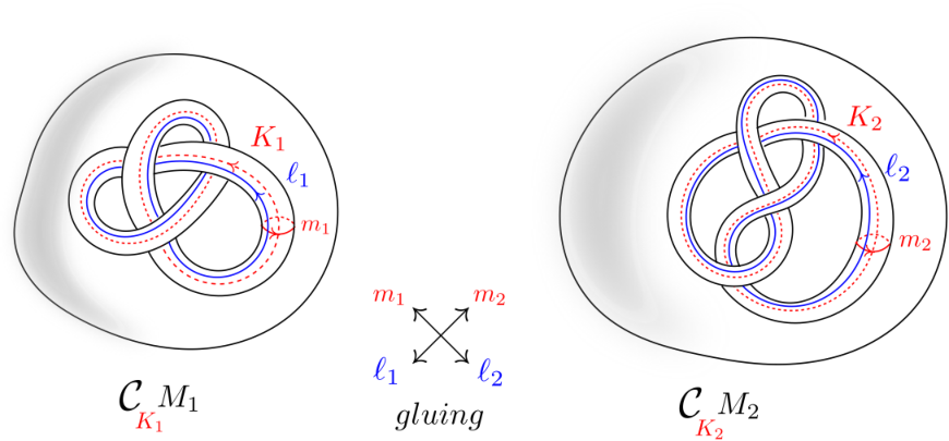
As mentioned by Gordon in [19, Section 6], the previous property had been noticed by Dehn in his 1907 paper [13] for a pair of three-dimensional spheres. The following terminology describing the operation performed in 2.19 is due to Siebenmann [74]:

2.20.

Let $M_{1}$ and $M_{2}$ be two oriented $\mathbb{Z}\!\operatorname{HS}$ ’s and let $K_{i}\subset M_{i}$ be oriented knots in them. Then, the oriented three-manifold $\boxed{(M_{1},K_{1})\oplus(M_{2},K_{2})}$ obtained by the procedure described in 2.19 is called the splice of $M_{1}$ and $M_{2}$ along the knots $K_{1}$ and $K_{2}$ .

The splicing operation is sketched in Figure 1. The meridians are denoted by $m_{1}$ and $m_{2}$ , whereas the longitudes are indicated by $\ell_{1}$ and $\ell_{2}$ . The curves in the figure are schematic, i.e., they should not be interpreted as linear projections of knots in the standard sphere. Otherwise, the knot $l_{i}$ would not be a longitude of $K_{i}$ , as their linking number would not be zero.

In the same article [74] in which he had introduced the splicing terminology, Siebenmann considered the special class of $\mathbb{Z}\!\operatorname{HS}$ ’s obtained from several Seifert-fibered ones by splicing them recursively along fibers of their respective Seifert fibrations. He encoded the resulting oriented $\mathbb{Z}\!\operatorname{HS}$ ’s by special types of decorated trees called splice diagrams, which we now discuss. We start by recalling some standard terminology from graph theory:

2.21.

A tree $T$ is a finite acyclic connected graph. The valency of a vertex $v$ is the number of edges incident to it, which we denote by $\boxed{\delta_{v}}$ . When $T$ has at least two vertices, the leaves of $T$ are those vertices of valency one, and the nodes of $T$ are the remaining vertices. If $T$ is a singleton, its unique vertex is taken to be a leaf. An edge joining two nodes is called internal.

2.22.

A splice diagram is a finite tree without vertices of valency two, such that for each node $v$ , every incident edge $e$ is decorated by a positive integer $\boxed{d_{v,e}}$ in the neighborhood of $v$ and such that around each node, the integers decorating adjacent edges are pairwise coprime. A star-shaped splice diagram is a splice diagram with a single node.

Siebenmann’s work [74] associates an oriented integral homology sphere to every splice diagram by an explicit procedure, which we now recall:

2.23.

Let $\Gamma$ be a splice diagram. Its associated oriented integral homology sphere $\boxed{\Sigma(\Gamma)}$ is constructed as follows:

•

For each node $v$ of $\Gamma$ , let $\boxed{\Gamma^{v}}$ be the star-shaped splice diagram obtained by taking the union of the compact edges of $\Gamma$ containing $v$ and by keeping only their decorations around $v$ .
•

If $(p_{1}(v),\dots,p_{\delta_{v}}(v))$ is the sequence of decorations on the edges of $\Gamma^{v}$ (arbitrarily ordered), consider the Seifert-fibered integral homology sphere $\boxed{\Sigma(\Gamma^{v})}:=\Sigma(p_{1}(v),\dots,p_{\delta_{v}}(v))$ (see 2.10 and 2.11), with its fibers oriented arbitrarily, but in a continuous way. The manifold $\Sigma(\Gamma^{v})$ has a set of $\delta_{v}$ distinguished fibers in bijection with the set of edges of $\Gamma$ adjacent to $v$ .
•

Given two adjacent nodes $u$ and $v$ of $\Gamma$ , splice $\Sigma(\Gamma^{u})$ and $\Sigma(\Gamma^{v})$ along the oriented fibers corresponding to the unique edge of $\Gamma$ joining $u$ and $v$ .
•

Perform the previous splicing simultaneously on the disjoint union of all oriented Seifert-fibered integral homology spheres with oriented fibers $\Sigma(\Gamma^{v})$ , indexed by all nodes $v$ of $\Gamma$ .
•

The resulting oriented integral homology sphere is $\Sigma(\Gamma)$ .

2.24.

Siebenmann’s construction is more general and allows negative edge weights on splice diagrams. We focus on the case of positive weights since this restriction is enough for describing the singularity links which are $\mathbb{Z}\!\operatorname{HS}$ ’s (see Theorem 2.26).

Theorem 2.12shows that all integral homology spheres associated to star-shaped splice diagrams occur as links of normal surface singularities. The notion of edge determinant, introduced formally by Neumann and Wahl in [61, Section 1] (although it appears already in [15, page 82]), allows to characterize which integral homology spheres may be realized as such links (see Theorem 2.26):

2.25.

Let $\Gamma$ be a splice diagram. If $u$ and $v$ are two adjacent nodes of $\Gamma$ , then the edge determinant of the edge $[u,v]$ is the number obtained by subtracting from the product of the two decorations on $[u,v]$ the product of the remaining decorations in the neighborhoods of $u$ and $v$ . We say that $\Gamma$ satisfies the edge determinant condition if the edge determinant of every internal edge of $\Gamma$ is positive.

We illustrate this definition with the running example from [61, Section 1]:

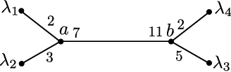
2.25.

Consider the splice diagram with two nodes and four leaves seen in Figure 2. It satisfies the edge determinant condition, as the edge determinant of its single internal edge is $7\cdot 11-(2\cdot 3)\cdot(5\cdot 2)=11>0$ .

In [15, Theorem 9.4], Eisenbud and Neumann gave an explicit description of all integral homology spheres that can be realized as surface singularity links. Here is the precise statement:

2.26.

The links of normal surface singularities which are $\mathbb{Z}\!\operatorname{HS}$ ’s are precisely the oriented three-manifolds $\Sigma(\Gamma)$ associated to splice diagrams which satisfy the edge determinant condition. Moreover, the diagram $\Gamma$ is completely determined by the link if for every non-internal edge $e$ of $\Gamma$ joining a node $v$ to a leaf $\lambda$ we have $d_{v,e}\geq 2$ .

Note that Theorem 2.12 shows that the Seifert fibered $\mathbb{Z}\!\operatorname{HS}$ ’s are not only surface singularity links, but they occur as links of isolated complete intersection singularities. This observation leads to the following natural analog of 1 stated in Section 1:

3.

Which integral homology spheres of the form $\Sigma(\Gamma)$ can occur as links of isolated complete intersection singularities?

Although a complete answer to this question remains unknown, a partial answer was given by Neumann and Wahl in [62]. Indeed, they showed that $\Sigma(\Gamma)$ is the link of an isolated complete intersection singularity whenever $\Gamma$ satisfies a supplementary hypothesis called the semigroup condition, which we now recall. We start with the auxiliary notions of linking number between two vertices and of degree of a node of $\Gamma$ :

2.27.

Let $\Gamma$ be a splice diagram. For every pair of vertices $u$ and $v$ of $\Gamma$ , their linking number $\boxed{\ell_{u,v}}$ is the product of edge weights adjacent to the shortest path $[u,v]$ on $\Gamma$ joining $u$ and $v$ . In particular, the degree of a node $v$ is the product $\boxed{d_{v}}:=\ell_{v,v}$ of all edge decorations adjacent to $v$ .

2.28.

The name linking number used for the integers $\ell_{u,v}$ is motivated by the fact that they agree with the linking numbers (inside the integral homology sphere $\Sigma(\Gamma)$ from 2.23) of the knots corresponding to the generic fibers of the Seifert fibered manifolds $\Sigma(\Gamma^{u})$ and $\Sigma(\Gamma^{v})$ . For more details, we refer to [15, Theorem 10.1]. Note that the edge determinant of an internal edge $[u,v]$ is positive if and only if $d_{u}d_{v}>\ell_{u,v}^{2}$ .

2.29.

Let $\Gamma$ be a splice diagram. Fix a node $v$ and an edge $e$ of $\Gamma$ adjacent to it. We say that $\Gamma$ satisfies the semigroup condition at $v$ in the direction of $e$ if $d_{v}$ belongs to the subsemigroup of $(\mathbb{N},+)$ generated by the positive integers $\ell_{v,\lambda}$ , where $\lambda$ varies among the leaves of $\Gamma$ seen from $v$ in the direction of $e$ (i.e., such that $e$ lies in the shortest path $[v,\lambda]$ ). If this condition is verified for all pairs $(v,e)$ , then we say that $\Gamma$ satisfies the semigroup condition.

2.30.

The semigroup condition is essential to extend the construction of Brieskorn-Pham-Hamm systems from star-shaped diagrams to arbitrary ones: it specifies how to replace the power of a single variable (indexed by the corresponding leaf) by a monomial in the variables indexed by leaves seen from $v$ in the direction of $e$ . Polynomials constructed in this way will be homogeneous relative to suitable weight vectors, described in 2.35 (1) below.

2.30.

As in Subsection 2.2, we consider the splice diagram $\Gamma$ from Figure 2. Note that $d_{a}=2\cdot 3\cdot 7=42$ , $\ell_{a,\lambda_{3}}=2\cdot 3\cdot 2=12$ , $\ell_{a,\lambda_{4}}=2\cdot 3\cdot 5=30$ , $d_{b}=2\cdot 5\cdot 11=110$ , $\ell_{b,\lambda_{1}}=2\cdot 5\cdot 3=30$ , and $\ell_{b,\lambda_{2}}=2\cdot 5\cdot 2=20$ . Therefore, $\Gamma$ satisfies the semigroup condition, as $d_{a}\in\mathbb{N}\langle\ell_{a,\lambda_{3}},\ell_{a,\lambda_{4}}\rangle$ and $d_{b}\in\mathbb{N}\langle\ell_{b,\lambda_{1}},\ell_{b,\lambda_{2}}\rangle$ . More precisely,

(2.5)

d_{a}=42=12+30=\ell_{a,\lambda_{3}}+\ell_{a,\lambda_{4}}\hskip 10.00002pt\text{ and }\hskip 10.00002ptd_{b}=110=30+4\cdot 20=\ell_{b,\lambda_{1}}+4\,\ell_{b,\lambda_{2}}.

Note that the semigroup condition is always satisfied at a node $v$ in the direction of an edge joining $v$ to a leaf. For instance, $d_{a}=42=2\cdot(3\cdot 7)=2\cdot\ell_{a,\lambda_{1}}\in\mathbb{N}\langle\ell_{a,\lambda_{1}}\rangle$ .

The following result is due to Neumann and Wahl (as a consequence of [61, Theorems 2.6 and 7.2]):

2.31.

Let $\Gamma$ be a splice diagram with $n$ leaves which satisfies the determinant and semigroup conditions. Then, there exists an isolated complete intersection singularity embedded in $\mathbb{C}^{n}$ whose oriented link is orientation-preserving homeomorphic to $\Sigma(\Gamma)$ .

In fact, Neumann and Wahl’s result referenced above is more general, since it concerns splice diagrams whose edge weights around vertices are not necessarily pairwise coprime. The reader interested in learning more about them and the associated splice quotient singularities may consult Wahl’s surveys [82, 83].

The proof of Theorem 2.31 is constructive. Indeed, given any splice diagram $\Gamma$ satisfying the semigroup condition, Neumann and Wahl build a family of systems of formal power series in $n$ variables which define equisingular isolated complete intersection singularities with link $\Sigma(\Gamma)$ (see Theorem 2.38). The explicit construction of such splice type systems and the associated splice type singularities will be discussed in Subsection 2.3 below. The largest class known up to date of complete intersection isolated surface singularities with integral homology sphere links remains that of splice type.

2.3. Splice type singularities

In this subsection we recall Neumann and Wahl’s construction of splice type systems [61, 62] associated to splice diagrams satisfying both the determinant and semigroup conditions (see Definitions 2.22, 2.25 and 2.29). Such systems define the so-called splice type singularities (see 2.34). For a description of how Neumann and Wahl were led to this construction, we refer the reader to Wahl’s paper [83].

Let $\boxed{\mathring{V}({\Gamma})}$ be the set of nodes of the splice diagram $\Gamma$ and $\boxed{\partial\,\Gamma}$ be its set of leaves. We denote by $\boxed{n}$ the number of leaves of $\Gamma$ . Following 2.23 we let $\boxed{\Gamma^{v}}$ be the star of a vertex $v$ of $\Gamma$ , i.e. the collection of all edges adjacent to $v$ , with inherited weights around $v$ . It contains precisely $\delta_{v}$ edges, i.e., as many as the valency of $v$ . In addition to the notion of linking number between pairs of vertices introduced in 2.27, it will often be convenient to work with the following related notion, first introduced in [61, Section 1]:

2.32.

The reduced linking number $\boxed{\ell_{v,u}^{\prime}}$ is defined as the product of all weights adjacent to the path $[u,v]$ excluding those around $u$ and $v$ . In particular, $\ell_{v,v}^{\prime}=1$ for each node $v$ of $\Gamma$ .

2.33.

Given a node $v$ and a leaf $\lambda$ of $\Gamma$ , it is immediate to check that $\ell_{v,\lambda}\,{d_{v,\lambda}}=\ell_{v,\lambda}^{\prime}\,d_{v}$ . This implies that the semigroup condition from 2.29 for the pair $(v,e)$ is satisfied if, and only if, $d_{v,e}$ belongs to the subsemigroup of $(\mathbb{N},+)$ generated by $\ell_{v,\lambda}^{\prime}$ , where $\lambda$ varies among the leaves of $\Gamma$ which are seen from $v$ in the direction of $e$ .

In what follows, we recall some standard notations from toric geometry. They are not required to define splice type singularities (and were not used in the foundational papers of Neumann and Wahl) but they are essential for our proof of the Milnor fiber conjecture.

Each leaf $\lambda$ of $\Gamma$ yields a variable $\boxed{z_{\lambda}}$ . Let $\boxed{M(\partial\,\Gamma)}$ be the lattice of exponent vectors of monomials in the variables $z_{\lambda}$ . We denote by $\boxed{N(\partial\,\Gamma)}$ its dual lattice of weight vectors of the variables $z_{\lambda}$ . We write the associated pairing using dot product notation, i.e. $\boxed{w\cdot m}\in\mathbb{Z}$ whenever $w\in N(\partial\,\Gamma)$ and $m\in M(\partial\,\Gamma)$ . The canonical basis $\{\boxed{w_{\lambda}}:\lambda\in\partial\,\Gamma\}$ of $N(\partial\,\Gamma)$ and the dual basis $\{\boxed{m_{\lambda}}:\lambda\in\partial\,\Gamma\}$ of $M(\partial\,\Gamma)$ identify both lattices with $\mathbb{Z}^{n}$ . Each node $v$ of $\Gamma$ has an associated weight vector

(2.6)

\boxed{w_{v}}:=\sum_{\lambda\in\partial\,\Gamma}\ell_{v,\lambda}\,w_{\lambda}\in N(\partial\,\Gamma).

If $v$ is a node of $\Gamma$ and $e\in\Gamma^{v}$ , we denote by $\boxed{\partial_{v,e}\Gamma}$ the set of leaves $\lambda$ of $\Gamma$ seen from $v$ in the direction of $e$ . The diagram $\Gamma$ satisfies the semigroup condition if, and only if, for each node $v$ , edge $e\in\Gamma^{v}$ and leaf $\lambda\in\partial_{v,e}\Gamma$ , there exists $\boxed{m_{v,e,\lambda}}\in\mathbb{N}$ such that:

(2.7)

d_{v}=\sum_{\lambda\in\partial_{v,e}\Gamma}m_{v,e,\lambda}\,\ell_{v,\lambda}\,,\hskip 10.00002pt\text{ or equivalently }\hskip 10.00002ptd_{v,e}=\sum_{\lambda\in\partial_{v,e}\Gamma}m_{v,e,\lambda}\,\ell_{v,\lambda}^{\prime}.

This last equivalence is a direct consequence of 2.33.

We use the coefficients from (2.7) to define an element of $M(\partial\,\Gamma)$ for each pair $(v,e)$ :

(2.8)

\boxed{m_{v,e}}:=\sum_{\lambda\in\partial_{v,e}\Gamma}m_{v,e,\lambda}\,m_{\lambda}\in M(\partial_{v,e}\Gamma)\subset M(\partial\,\Gamma).

Following [61], we refer to it as an admissible exponent vector for $(v,e)$ . By (2.7), it satisfies

(2.9)

w_{v}\cdot m_{v,e}=d_{v}\hskip 10.00002pt\text{ for each edge }\;e\in\Gamma^{v}.

In turn, each admissible exponent vector $m_{v,e}$ defines an admissible monomial:

(2.10)

\boxed{\underline{z}^{m_{v,e}}}:=\prod_{\lambda\in\partial_{v,e}\Gamma}z_{\lambda}^{m_{v,e,\lambda}}.

The next definition is a reformulation of a notion introduced by Neumann and Wahl in [61, Section 2]:

2.34.

Let $\Gamma$ be a splice diagram which satisfies both the determinant and semigroup conditions, and assume that the set of $n$ leaves of $\Gamma$ is totally ordered. For each node $v$ and adjacent edge $e$ of it, fix an admissible exponent vector $m_{v,e}\in M(\partial\Gamma)$ defined in (2.8).

•

A strict splice type system for $\Gamma$ is a finite family of $(n-2)$ polynomials of the form

(2.11)

\boxed{f_{v,i}(\underline{z})}:=\sum_{e\in{\operatorname{Star}(v)}}\!\!\!\!\boxed{c_{v,e,i}}\;\underline{z}^{m_{v,e}}\hskip 10.00002pt\text{for all }i\in\{1,\dots,\delta_{v}-2\}\,\text{ and }\text{ each node }v\text{ of }\Gamma.

We require the coefficients $c_{v,e,i}$ to satisfy the Hamm determinant condition. Namely, for any node $v\in\Gamma$ , and any fixed ordering of the edges in $\Gamma^{v}$ , all the maximal minors of the matrix of coefficients $(c_{v,e,i})_{e,i}\in\mathbb{C}^{\delta_{v}\times(\delta_{v}-2)}$ must be non-zero.

•

A splice type system $\boxed{\mathcal{S}(\Gamma)}$ associated to $\Gamma$ is a finite family of power series of the form

(2.12)

\boxed{F_{v,i}(\underline{z})}:=f_{v,i}(\underline{z})+g_{v,i}(\underline{z})\hskip 10.00002pt\text{for all }i\in\{1,\dots,\delta_{v}-2\}\,\text{ and any fixed node }v\text{ of }\Gamma,

where the collection $(f_{v,i})_{v,i}$ is a strict splice type system for $\Gamma$ and each $g_{v,i}$ is a convergent power series near the origin satisfying the following condition for each exponent vector $m$ in its support:

(2.13)

w_{v}\cdot m>d_{v}.

•

A splice type singularity associated to $\Gamma$ is the subgerm of $(\mathbb{C}^{n},0)$ defined by a splice type system $\mathcal{S}(\Gamma)$ .

2.35.

The following observations regarding 2.34 are in order:

(1)

By equations (2.9) and (2.13), each polynomial $f_{v,i}$ is $w_{v}$ -homogeneous, where $w_{v}$ is the weight vector from (2.6), and each monomial appearing in $g_{v,i}$ has higher $w_{v}$ -weight.
(2)

The first appearance of splice type systems can be traced back to [60]. In that paper, the edge weights around nodes were not assumed to be pairwise coprime, but the edge determinant and semigroup conditions were still required. Neumann and Wahl proved that under a supplementary condition (called the congruence condition), it is possible to pick the series $F_{v,i}(\underline{z})$ in an equivariant way under the action of certain finite abelian groups. This construction then leads to defining splice quotient singularities as the quotients of the associated splice type singularities by those abelian groups. These singularities and their defining systems are studied thoroughly in [62] (see also Wahl’s surveys [82, 83]).
(3)

Neumann and Wahl proved in [62] that the set of splice-type subgerms of $\mathbb{C}^{n}$ corresponding to a given splice diagram satisfying the determinant and the semigroup condition is independent of the choice of admissible exponents. For a detailed proof, we refer the reader to [12, Theorem 9.1].

The following two examples illustrate 2.34:

2.35.

Consider the splice diagram from Figure 2. As shown in Examples 2.2 and 2.2, $\Gamma$ satisfies the determinant and semigroup conditions. The explicit semigroup membership identities from (2.5) yield the following associated strict splice type system:

f_{a}:=z_{1}^{2}-z_{2}^{3}+z_{3}z_{4}\hskip 10.00002pt\text{ and }\hskip 10.00002ptf_{b}:=z_{1}z_{2}^{4}+z_{3}^{5}-z_{4}^{2}.

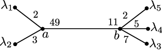
Another possible choice for the $w_{b}$ -homogeneous function $f_{b}$ is $z_{1}^{3}z_{2}+z_{3}^{5}-z_{4}^{2}$ , obtained by replacing the admissible monomial $z_{1}z_{2}^{4}$ by the other possible admissible monomial $z_{1}^{3}z_{2}$ for $(b,[b,a])$ . This second monomial is admissible because $d_{b}=110=3\cdot 30+1\cdot 20=3\cdot\ell_{b,\lambda_{1}}+1\cdot\ell_{b,\lambda_{2}}$ ).

2.35.

Consider the splice diagram $\Gamma$ from Figure 3 with nodes $a$ and $b$ . Then, $d_{a}=294$ , $d_{b}=770$ and $\ell_{a,b}=420$ , so $d_{a}\,d_{b}>\ell_{a,b}^{2}$ . Therefore, the edge determinant condition holds for $[a,b]$ by 2.28. Furthermore,

49=0\cdot(2\cdot 5)+1\cdot(2\cdot 7)+1\cdot(5\cdot 7)\hskip 10.00002pt\text{ and }\hskip 10.00002pt11=1\cdot(3)+4\cdot(2)=3\cdot(3)+1\cdot(2),

so the semigroup condition is also satisfied. Associated admissible exponent vectors are $m_{a,[a,b]}=(0,0,0,1,1)$ and $m_{b,[a,b]}=(1,4,0,0,0)$ or $(3,1,0,0,0)$ . The following polynomials determine a strict splice type system for $\Gamma$ :

\begin{cases}f_{a,1}:=\;\;\;\,z_{1}^{2}\;\;\;-\;\;\;2\;z_{2}^{3}\;+\;\;\;z_{4}\,z_{5},\\ f_{b,1}:=\;\;\;\;z_{1}z_{2}^{4}+z_{3}^{7}+\;\;z_{4}^{5}\,-\;2155\;z_{5}^{2},\\ f_{b,2}:=33\,z_{1}z_{2}^{4}+z_{3}^{7}+2\,z_{4}^{5}-\;2123\,z_{5}^{2}.\,\end{cases}

An alternative system is obtained by replacing the admissible monomial $z_{1}z_{2}^{4}$ in $f_{b,1}$ and $f_{b,2}$ with $z_{1}^{3}z_{2}$ .

2.36.

Our paper [12] describes standard tropicalizing fans of splice type singularities in the sense of 5.4, and shows that splice type systems are Newton non-degenerate complete intersection presentations of them in the sense of 5.9. These results are essential tools to prove analogous facts for their edge-deformations, introduced in Section 6 (see also 6.8). The weight vectors $(w_{v})_{v}$ indexed by the nodes of $\Gamma$ generate the positive rays of the standard tropicalizing fan of the splice type singularity. Its remaining rays are generated by the basis vectors $(w_{\lambda})_{\lambda}$ of $N(\partial\,\Gamma)$ . Moreover, the associated splice diagram appears as a transversal section of the local tropicalization of a splice type singularity (see [12, Theorem 1.2]). This gives the first tropical interpretation of splice diagrams, whenever they satisfy the determinant and semigroup conditions. We make use of this fact in Step (5) of Section 7.

2.37.

Let $(X,o)$ be a splice type singularity associated to the splice diagram $\Gamma$ . For each leaf $\lambda$ of $\Gamma$ , one may consider the hyperplane section of $(X,o)$ by the hyperplane of coordinates defined by $z_{\lambda}=0$ . As a particular case of Neumann and Wahl’s theorem [62, Theorem 7.2 (6)], this hyperplane section is an irreducible germ of curve, therefore its associated link is a knot inside the link of $(X,o)$ . This fact will be used in 2.39.

In [61, Theorems 2.6 and 7.2], Neumann and Wahl prove the following explicit form of Theorem 2.31:

2.38.

Let $\Gamma$ be a splice diagram which satisfies both the determinant and the semigroup conditions. Then the link of any splice type singularity associated to $\Gamma$ is orientation-preserving homeomorphic to $\Sigma(\Gamma)$ .

2.4. Neumann and Wahl’s Milnor fiber conjecture

In this subsection we explain Neumann and Wahl’s four-dimensional splicing operation (see 2.39) and we give a more precise formulation of the Milnor fiber conjecture that the one given in the Introduction (see 2.41). We conclude by stating a corollary of our proof of this conjecture (see Theorem 2.42).

Throughout this subsection, we fix a splice diagram $\Gamma$ with $n$ leaves satisfying the determinant and the semigroup conditions (see Definitions 2.25 and 2.29). Furthermore, we assume that $\Gamma$ is not star-shaped and we fix two adjacent nodes $\boxed{a,b}$ of it. As illustrated in Figure 4, we let $\boxed{\Gamma_{a}}$ and $\boxed{\Gamma_{b}}$ be the splice diagrams obtained by cutting $\Gamma$ at an interior point $\boxed{r}$ of $[a,b]$ . Denote by $\boxed{r_{a}}\in\Gamma_{a}$ and $\boxed{r_{b}}\in\Gamma_{b}$ the corresponding leaves of $\Gamma_{a}$ and $\Gamma_{b}$ . We view them as roots of the two trees. We let $\boxed{n_{a}}$ and $\boxed{n_{b}}$ be the number of leaves of $\Gamma_{a}$ and $\Gamma_{b}$ , respectively. Therefore, $n=n_{a}+n_{b}-2$ .

It is a simple matter to check that $\Gamma_{a}$ and $\Gamma_{b}$ also satisfy the determinant and semigroup conditions. Thus, we may use the three splice diagrams $\Gamma$ , $\Gamma_{a}$ and $\Gamma_{b}$ to build three splice type systems. We let $\boxed{X}$ , $\boxed{X_{a}}$ and $\boxed{X_{b}}$ be the germs at the origin defined by each system in $\mathbb{C}^{n}$ , $\mathbb{C}^{n_{a}}$ and $\mathbb{C}^{n_{b}}$ , respectively. We denote by $x_{\lambda}$ the variables of the ambient space $\mathbb{C}^{n_{a}}$ of $X_{a}$ and by $y_{\mu}$ those of the ambient space $\mathbb{C}^{n_{b}}$ of $X_{b}$ , where $\lambda$ varies in the set $\partial\,\Gamma_{a}$ of leaves of $\Gamma_{a}$ and $\mu$ varies in the set $\partial\,\Gamma_{b}$ of leaves of $\Gamma_{b}$ . In particular, there are two variables, $x_{r_{a}}$ and $y_{r_{b}}$ , which correspond to the roots of the two trees.

Since the germs $X$ , $X_{a}$ , and $X_{b}$ are isolated complete intersections, they have well-defined Milnor fibers $\boxed{F}$ , $\boxed{F_{a}}$ , $\boxed{F_{b}}$ , which are compact oriented four-dimensional manifolds with boundary. Furthermore, their boundaries are orientation-preserving diffeomorphic to the links of the associated singularities. The Milnor fiber conjecture of Neumann and Wahl describes a concrete topological operation to build $F$ from $F_{a}$ and $F_{b}$ . In what follows, we review this construction.

Consider the restriction of the coordinate function $x_{r_{a}}$ to $X_{a}$ . This holomorphic function has an isolated critical point at $0\in X_{a}$ . Therefore, it defines an open book (a terminology introduced by Winkelnkemper [84], also called an open book decomposition) on the link $\partial(X_{a},0)$ of $(X_{a},0)$ : it is the Milnor open book induced by the argument of the holomorphic function (see [43, Section 6.5]). Since the link $\partial(X_{a},0)$ is diffeomorphic to the boundary of the Milnor fiber $F_{a}$ , we obtain an open book on this boundary [24]. Denote by $\boxed{G_{a}}\hookrightarrow F_{a}$ a compact surface with boundary obtained by pushing a page of this open book inside $F_{a}$ , while keeping the boundary fixed. Figure 5 depicts this construction in lower dimension. Note that the boundary of $G_{a}$ is connected, because the hyperplane sections of $X_{a}$ by coordinate hyperplanes are irreducible (see 2.37).

We let $N_{F_{a}}(G_{a})$ be a tubular neighborhood of $G_{a}$ in $F_{a}$ . Consider the associated classical cut $\mathcal{C}_{G_{a}}F_{a}$ of $F_{a}$ along $G_{a}$ , as in 2.17. Note that the normal bundle of $G_{a}$ inside $F_{a}$ is trivial because it is a disk bundle over a connected surface with non-empty boundary. Therefore, the tubular neighborhood $N_{F_{a}}(G_{a})$ is diffeomorphic to $G_{a}\times\mathbb{D}$ , where $\mathbb{D}$ denotes a compact two-dimensional disk. This implies that the longitudinal boundary of $N_{F_{a}}(G_{a})$ , which we define as

(2.14)

\boxed{\partial_{long}N_{F_{a}}(G_{a})}:=\mathcal{C}_{G_{a}}F_{a}\cap N_{F_{a}}(G_{a})\hookrightarrow\partial_{top}(\mathcal{C}_{G_{a}}F_{a})

is diffeomorphic to $G_{a}\times\mathbb{S}^{1}$ .

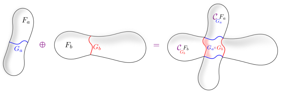
The next definition recalls Neumann and Wahl’s four-dimensional splicing operation in this context (see [61, Section 6] for further details). The construction is depicted in Figure 6.

2.39.

Let $(F_{a},G_{a})$ and $(F_{b},G_{b})$ be the pairs defined above. The manifold $\boxed{(F_{a},G_{a})\oplus(F_{b},G_{b})}$ obtained by splicing $F_{a}$ and $F_{b}$ along $G_{a}$ and $G_{b}$ is constructed from the disjoint union

\mathcal{C}_{G_{a}}F_{a}\>\>\sqcup\>\>(G_{a}\times G_{b})\>\>\sqcup\>\>\mathcal{C}_{G_{b}}F_{b}

by identifying $G_{a}\times\mathbb{S}^{1}\simeq\partial_{long}N_{F_{a}}(G_{a})\hookrightarrow\mathcal{C}_{G_{a}}F_{a}$ with $G_{a}\times\mathbb{S}^{1}\simeq G_{a}\times\partial_{top}G_{b}\hookrightarrow G_{a}\times G_{b}$ and, similarly, $G_{b}\times\mathbb{S}^{1}\simeq\partial_{long}N_{F_{b}}(G_{b})\hookrightarrow\mathcal{C}_{G_{b}}F_{b}$ with $\mathbb{S}^{1}\times G_{b}\simeq\partial_{top}G_{a}\times G_{b}\hookrightarrow G_{a}\times G_{b}$ .

A basic, yet crucial, property of this operation is that it induces the $3$ -dimensional splicing operation of 2.20 at the level of boundaries. As no proof for this fact was given in [61], we include one below.

2.40.

Let $(F_{a},G_{a})$ and $(F_{b},G_{b})$ be pairs as above. Then, the boundary of the manifold obtained by splicing $F_{a}$ and $F_{b}$ along $G_{a}$ and $G_{b}$ is the three-dimensional manifold obtained by splicing their boundaries. More precisely, we have an orientation preserving diffeomorphism:

\partial_{top}\left((F_{a},G_{a})\oplus(F_{b},G_{b})\right)\simeq(\partial_{top}F_{a},\partial_{top}G_{a})\oplus(\partial_{top}F_{b},\partial_{top}G_{b}).

Proof.

Let $(F,G)$ be one of the pairs $(F_{a},G_{a})$ and $(F_{b},G_{b})$ . The next reasoning is to be followed along using Figure 7, suggestive of an analogous situation in one dimension lower.

As explained above, the boundary $K$ of the surface $G$ is a knot in $\partial_{top}F$ , because the hyperplane sections of splice type singularities by coordinate hyperplanes are irreducible. We must show that the trivialization of the circle bundle $\partial_{top}N_{\partial_{top}F}(K)\to K$ induced by the chosen trivialization of the circle bundle $\partial_{long}N_{F}(G)\to G$ coincides up to isotopy with the trivialization described in 2.4. Thus, we must check that the boundary of a constant section of $\partial_{long}N_{F}(G)\to G$ relative to this trivialization has linking number $0$ with $K$ inside $\partial_{top}F$ .

Consider a page $G_{K}\hookrightarrow\partial_{top}F$ of the given open book on $\partial_{top}F$ with binding $K$ . As $G$ is obtained by pushing $G_{K}$ inside $F$ while preserving its boundary, $G\cup G_{K}$ is the boundary of an oriented compact three-manifold $M$ diffeomorphic to a handelbody and embedded in $F$ . We choose the tubular neighborhood $N_{\partial_{top}F}(K)$ to be transversal to $M$ . Therefore, the intersection $\partial_{top}N_{\partial_{top}F}(K)\ \cap\ M$ is a section of the circle bundle $\partial_{top}N_{\partial_{top}F}(K)\to K$ . Slightly turning this intersection inside each fiber yields another section $G^{\prime}$ which is disjoint from $M$ . Therefore, its boundary $K^{\prime}:=G^{\prime}\ \cap\ \partial_{top}F\hookrightarrow\partial_{top}F$ is disjoint from $G_{K}=M\ \cap\ \partial_{top}F$ . This implies that $lk_{\partial_{top}F}(K^{\prime},K)=0$ , as we wanted to show. ∎

2.39allows us to present a more precise version of Neumann and Wahl’s Milnor fiber conjecture of [61, Section 6] than the one given in Section 1:

2.41.

Let $X$ be a splice type singularity whose splice diagram $\Gamma$ is not star-shaped. Fix an internal edge $[a,b]$ of $\Gamma$ . Let $\Gamma_{a}$ and $\Gamma_{b}$ be the rooted splice diagrams obtained by cutting $\Gamma$ at an interior point of $[a,b]$ . Denote by $X_{a}$ and $X_{b}$ the splice type singularities associated to $\Gamma_{a}$ and $\Gamma_{b}$ . Let $F$ , $F_{a}$ and $F_{b}$ be Milnor fibers of $X$ , $X_{a}$ and $X_{b}$ , respectively. Consider a surface $G_{a}\hookrightarrow F_{a}$ obtained as above from the open book defined on $\partial(X_{a},0)$ by the variable associated to the root of $\Gamma_{a}$ . Consider an analogous surface $G_{b}\hookrightarrow F_{b}$ . Then, $F$ is homeomorphic to the result of splicing $F_{a}$ and $F_{b}$ along $G_{a}$ and $G_{b}$ .

As was mentioned in Section 1, the formulation of this conjecture was motivated by the Casson invariant conjecture from [59]. In [61, Section 6], Neumann and Wahl proved that the Casson invariant conjecture for splice type singularities follows from the Milnor fiber conjecture. So far, the latter has only been confirmed in special cases. Indeed, Neumann and Wahl [61, Section 8] showed it for hypersurface singularities defined by equations of the form $z^{n}+f(x,y)=0$ , whereas Lamberson work [41] discusses a generalization of this class of singularities, whose links are obtained from $\mathbb{S}^{3}$ by iterated cyclic branched covers along suitable links.

Note that 2.41 presumes that all splice type singularities with a fixed splice diagram have homeomorphic Milnor fibers, since for a fixed $X$ , the singularity $X_{a}$ can be chosen to be any splice type singularity with diagram $\Gamma_{a}$ . Remarkably, this subtle yet previously unknown fact is a direct consequence of the proof of the conjecture outlined in this paper. More precisely, we have:

2.42.

The Milnor fibers of any two splice type singularities arising from the same splice diagram are diffeomorphic.

Proof.

The proof outline of the Milnor fiber conjecture discussed in Section 7 allows us to reduce to the case when the splice diagram $\Gamma$ is star-shaped. For such diagrams, our description of Milnor fibers through roundings shows that the Milnor fiber of such a splice type singularity does not depend of the higher order terms of the defining splice type system, but only on the initial Pham-Brieskorn-Hamm system (see 2.14).

It remains to check that the Milnor fibers of those singularities do not depend on the matrix of coefficients satisfying the Hamm determinant condition. But this is a consequence of the fact that those singularities are quasi-homogeneous. Indeed, quasi-homogeneity ensures that any Euclidean ball centered at the origin becomes a Milnor ball for all such systems simultaneously. This proves the statement. ∎

3. The main ideas of our proof

In this section we give an informal description of the main ideas involved in our proof of 2.41. In Subsection 3.1, we explain how to canonically decompose Milnor fibers into pieces using real oriented blowups of embedded resolutions of smoothings. In Subsection 3.2 we extend this construction to quasi-toroidalizations of suitable smoothings using the notion of rounding of a complex log space and explain how to construct quasi-toroidalizations using tropical geometry techniques. Finally, Subsection 3.3 gives some basic intuitions about local tropicalization and Newton non-degeneracy, two notions which are key players in our construction of quasi-toroidalizations of smoothings.

3.1. Canonical Milnor fibrations through real oriented blowups

In this subsection we explain how A’Campo’s notion of real oriented blow up yields canonical representatives of the Milnor fibrations over the circle of a given smoothing of an isolated singularity, once an embedded resolution of the smoothing is fixed.

Throughout, we let $(X,o)$ be an isolated singularity of arbitrary dimension and we let $f\colon(Y,o)\to(\mathbb{C},0)$ be a smoothing of $(X,o)$ . Consider an embedded resolution of $f$ , that is, a modification $\pi\colon\tilde{Y}\to Y$ which restricts to an isomorphism outside $o$ , such that $\tilde{Y}$ is smooth and the zero level set $Z(\tilde{f})$ of the lifting $\tilde{f}:=f\circ\pi$ of $f$ to $\tilde{Y}$ is a normal crossings divisor. It is natural to ask how the non-zero levels of $\tilde{f}$ degenerate to $Z(\tilde{f})$ . By definition, these levels are identified via $\pi$ with the Milnor fibers of $f$ . This produces a decomposition of those Milnor fibers into compact pieces, each piece consisting of the points which degenerate to a fixed irreducible component of $Z(\tilde{f})$ . These pieces are manifolds with corners, whose boundaries degenerate to the singular locus of $Z(\tilde{f})$ .

This decomposition into pieces is analogous to Mumford’s plumbed decomposition of the link of an isolated surface singularity obtained by looking at the way the link degenerates onto the exceptional divisor of a good resolution (see [52, Section 1]). As in that prototypical case, the decomposition of a given Milnor fiber of $f$ is not canonical, because it depends on the choices of embedded resolution, of suitable coordinate systems near the singular locus of the exceptional divisor and also of a level $f^{-1}(\lambda)$ of $f$ with $0<|\lambda|\ll 1$ .

Once the embedded resolution is fixed, the non-canonical aspect of the construction can be repaired via the operation of real oriented blowup, introduced by A’Campo in his study of monodromies of germs $f\colon(\mathbb{C}^{n+1},0)\to(\mathbb{C},0)$ [1, Section 2]. This operation may be performed starting from any normal crossings divisor $D$ (seen as a reduced hypersurface) in a complex manifold $W$ . Its effect is to determine a canonical cut of $W$ along $D$ , which contrasts with the dependency of a classical cut (see 2.17) on the choice of a tubular neighborhood. This canonical cut produces a real analytic manifold with corners $W_{D}$ , together with a map

\tau_{W,D}\colon W_{D}\to W.

This real oriented blowup map is proper and a homeomorphism on $W\setminus D$ . It sends the topological boundary $\partial_{top}W_{D}$ of $W_{D}$ onto $D$ and, furthermore, the corner locus of $W_{D}$ is the preimage of the singular locus of $D$ under $\tau_{W,D}$ . In this way, the algebro-geometric boundary $D$ of the pair $(W,D)$ (in algebraic geometry it is customary to say that a boundary is a divisor) is replaced by the topological boundary $\partial_{top}W_{D}$ of the piecewise-smooth manifold $W_{D}$ . Figure 8 shows a “real analog” of this procedure for a divisor $D$ with two components in a smooth surface.

3.0.

When $W=\mathbb{C}$ and $D$ is the origin, the real oriented blowup is the map $\tau_{\mathbb{C},\{0\}}\colon[0,+\infty)\times\mathbb{S}^{1}\to\mathbb{C}$ obtained through the use of polar coordinates: $(r,e^{i\theta})\to re^{i\theta}$ . The origin of $\mathbb{C}$ , seen as an algebro-geometric boundary, is replaced by the topological boundary circle $\mathbb{S}^{1}$ of the cylinder $[0,+\infty)\times\mathbb{S}^{1}$ . This example will be thoroughly discussed in Subsection 4.2.

Let us come back to the lifted morphism $\tilde{f}\colon\tilde{Y}\to\mathbb{C}$ defined earlier. Performing both the real oriented blowup of $\tilde{Y}$ along $Z(\tilde{f})$ and of $\mathbb{C}$ at the origin allows us to lift the function $\tilde{f}$ in a canonical way to those new spaces. Moreover, the restriction $\partial(\tilde{f})\colon\partial\tilde{Y}_{Z(\tilde{f})}\to\mathbb{S}^{1}$ of this lift to the boundaries of the source and target spaces gives a canonical representative of the Milnor fibration of $f$ above a circle, relative to its embedded resolution $\pi$ (see A’Campo’s [1, Section 2] and 4.52 of a theorem of Nakayama and Ogus).

Since the source space $\partial\tilde{Y}_{Z(\tilde{f})}$ is endowed with a canonical surjection

(3.1)

\tau_{\tilde{Y},Z(\tilde{f})}\colon\partial\tilde{Y}_{Z(\tilde{f})}\twoheadrightarrow Z(\tilde{f}),

we see that it inherits a canonical decomposition into pieces that are manifolds with corners. Each piece lies above an irreducible component of $Z(\tilde{f})$ . This yields the desired decomposition of all fibers of the canonical Milnor fibration $\partial(\tilde{f})$ .

3.2. Quasi-toroidalizations

In this subsection we introduce a class of maps called quasi-toroidalizations, associated to smoothings of isolated singularities, which are more general than the embedded resolutions $\pi\colon\tilde{Y}\to Y$ considered in Subsection 3.1, and which play a central role in our proof of 2.41. They may have mildly singular total spaces and special fibers which are not crossing normally. Remarkably, the construction of canonical Milnor fibrations from modifications explained in Subsection 3.1 can be applied to quasi-toroidalizations as well. This extension uses the operation of rounding, a generalization of real oriented blowups introduced by Kato and Nakayama [33] in the context of logarithmic geometry (in the sense of Fontaine and Illusie), or log geometry for short. The latter will be reviewed in Subsection 4.3. Quasi-toroidalizations are relevant for us, as the modifications induced by the natural fans we use in order to subdivide the local tropicalizations of our germs are quasi-toroidalizations. We could of course subdivide those fans even further, in a non-canonical way, until we reach an embedded resolution morphism. However, this process would fail to describe our morphisms explicitly in terms of the given splice diagrams.

Let us start with the notions of toroidal varieties and morphisms:

3.1.

Let $(W,\partial W)$ be a pair consisting of an equidimensional complex analytic space $W$ and a reduced complex hypersurface $\partial W$ in it. We say that $(W,\partial W)$ is a toroidal variety or a toroidal pair if it is locally analytically isomorphic to the pair consisting of a toric variety and its toric boundary, i.e., the complement of its dense algebraic torus. Such a local isomorphism is a toric chart of the toroidal pair. The hypersurface $\partial W$ is called a toroidal boundary for $W$ .

If $(W,\partial W)$ is a toroidal pair, then the toroidal stratification of $W$ is obtained by gluing together using the toric charts the preimages of the various toric orbits.

A toroidal morphism is a complex analytic morphism $(V,\partial V)\to(W,\partial W)$ between toroidal varieties that is locally analytically a monomial map when restricted to convenient toric charts.

3.2.

The notion of toroidal variety generalizes that of a toric variety, since every pair consisting of a toric variety and its toric boundary is automatically toroidal. Note that $(W,\partial W)$ is a toroidal pair if and only if $W\smallsetminus\partial W\hookrightarrow W$ is a toroidal embedding in the sense of [36].

3.3.

Fix an isolated singularity $(X,o)$ of arbitrary dimension and a smoothing $f\colon(Y,0)\to(\mathbb{C},0)$ of it. A quasi-toroidalization of $f$ is a modification $\pi\colon\tilde{Y}\to Y$ satisfying the following conditions:

(1)

there exists a reduced hypersurface $\partial\tilde{Y}$ in $\tilde{Y}$ such that the lifting $\tilde{f}\colon(\tilde{Y},\partial\tilde{Y})\to(\mathbb{C},0)$ of $f$ to $\tilde{Y}$ is a toroidal morphism,
(2)

the zero-locus $Z(\tilde{f})$ of $\tilde{f}$ in $\tilde{Y}$ is included in the toroidal boundary $\partial\tilde{Y}$ , and
(3)

locally around each point $x$ of $\partial\tilde{Y}$ , we can find a (local) toroidal stratum $S$ for which the (local) irreducible components of $\partial\tilde{Y}$ containing $x$ that are not components of $Z(\tilde{f})$ are exactly those irreducible components of $\partial\tilde{Y}$ containing $S$ .

The third condition may seem strange at first sight. It originates in the observation that, unlike normal crossing divisors in manifolds (or smooth varieties), closed subdivisors of toroidal boundaries are not necessarily toroidal (see Examples 4.1 and 4.1). Its exact formulation is explained in 4.6.

3.4.

The relevance of quasi-toroidalizations for our work lies in the following crucial observation. Mimicking the real oriented blowup construction of the previous subsection in this more general context via Kato and Nakayama’s rounding operation (see Subsection 4.5) and restricting to $Z(\tilde{f})$ , produces a morphism

(3.2)

\partial(\tilde{f})\colon\partial\tilde{Y}_{|_{Z(\tilde{f})}}\to\mathbb{S}^{1}

which is a representative of the Milnor fibration of $f$ . This is a consequence (see 4.52) of a more general local triviality theorem for roundings proved by Nakayama and Ogus [53, Theorem 3.7], stated as Theorem 4.49 below.

In order to use quasi-toroidalizations to determine the topology of the Milnor fiber of a splice type singularity $(X,0)\hookrightarrow(\mathbb{C}^{n},0)$ , we must first pick an appropriate smoothing $f\colon(Y,0)\to(\mathbb{C},0)$ . Notice that, unlike the quasi-toroidalization $\pi\colon\tilde{Y}\to Y$ , the Milnor fiber is independent (up to diffeomorphism) of the choice of $f$ because $X$ is an isolated complete intersection, which implies by an important result of Tyurina [79, Theorem 8.1] (see also [44, Chapter 6] or [21, Theorem 1.16]) that its miniversal deformation has an irreducible (even smooth) base. Thus, we may pick a smoothing that is well-adapted to proving 2.41. We construct such a smoothing by deforming the splice type system defining $X$ in a way compatible with the given internal edge $[a,b]$ (see 6.3). The deformed system defines a three-dimensional germ $(Y,0)\hookrightarrow(\mathbb{C}^{n+1},0)$ .

The local tropicalization of this deformed system (a notion discussed in Subsection 3.3 and Section 5) is supported on a three-dimensional fan $\mathcal{F}$ contained in the cone of weights $(\mathbb{R}_{\geq 0})^{n+1}$ defining $\mathbb{C}^{n+1}$ as an affine toric variety. This fan has the following crucial property:

3.5.

Consider the toric birational morphism $\pi_{\mathcal{F}}\colon\mathcal{X}_{\mathcal{F}}\to\mathbb{C}^{n+1}$ defined by the fan $\mathcal{F}$ and let $\pi\colon\tilde{Y}\to Y$ be its restriction to the strict transform of $Y$ by $\pi_{\mathcal{F}}$ . Then, the map $\pi$ is a quasi-toroidalization of $f$ . Furthermore, the dual complex of the exceptional divisor $E:=\pi^{-1}(0)$ is naturally isomorphic to a subdivision of the splice diagram $\Gamma$ of $(X,0)\hookrightarrow(\mathbb{C}^{n},0)$ , obtained by adding an interior point $r$ of the edge $[a,b]$ as an extra node and subdividing $[a,b]$ accordingly.

The second part of 3.5 confirms that the quasi-toroidalization $\pi\colon\tilde{Y}\to Y$ of $f$ is adapted to the proof of 2.41. As we discuss in Step (8) of Section 7, this property yields a decomposition of the exceptional divisor $E$ into three pieces: two divisors $D_{a}$ and $D_{b}$ coming from the $a$ - and $b$ -sides, respectively, and an irreducible central divisor $D_{r}$ corresponding to the new vertex $r$ . Moreover, the special fiber $Z(\tilde{f})$ of $\tilde{f}$ is reduced, making $\tilde{f}$ analogous to a semistable degeneration in the sense of [36]. Its component $D_{r}$ is a cartesian product of two projective curves. In turn, this last fact then allows us to prove that the central piece of the Milnor fiber which connects the $a$ -side and $b$ -side has the desired product structure. This central piece is obtained by intersecting the preimage $\tau_{\tilde{Y},Z(\tilde{f})}^{-1}(D_{r})$ of the analog in our context of the map (3.1) with a fiber of the restriction map $\partial(\tilde{f})$ from (3.2). The product structure results from the reducedness of the special fiber $Z(\tilde{f})$ combined with a result of Achinger and Ogus [3, Corollary 4.1.9].

In a similar way, the $a$ -side piece of any Milnor fiber of $(X,0)$ is recovered by intersecting the preimage $\tau_{\tilde{Y},Z(\tilde{f})}^{-1}(D_{a})$ and the fibers of the restriction map $\partial(\tilde{f})$ from (3.2). This piece can then be identified with a Milnor fiber of a smoothing $f_{a}\colon(Y_{a},0)\to(\mathbb{C},0)$ of a convenient splice type singularity $(X_{a},0)$ associated to the $a$ -side rooted subtree $\Gamma_{a}$ of $\Gamma$ , cut (as explained in Subsection 2.4) along a pushed page of the Milnor open book defined by the root coordinate $x_{r_{a}}$ . The total space $Y_{a}$ is determined from the system defining $(Y,0)$ by its pullback under a suitable monomial map $\varphi_{a}\colon\mathbb{C}^{n_{a}+1}\to\mathbb{C}^{n+1}$ (see Steps (3) and (4) of Section 7). In turn, the smoothing $f_{a}$ is obtained by restricting $f\circ\varphi_{a}$ to $Y_{a}$ . This identification of portions of Milnor fibers of smoothings of distinct singularities is done using log geometry techniques. More concretely, we prove that the corresponding pieces of the canonical Milnor fibrations obtained through rounding are homeomorphic (see Steps (23) through (26) of Section 7).

Basic to the proof of this homeomorphism is the following reinterpretation of cutting the Milnor fibers of $(X_{a},0)$ in the direction of the root $r_{a}$ of $\Gamma_{a}$ . It can be achieved by cutting a level of the smoothing $f_{a}\colon(Y_{a},0)\to(\mathbb{C},0)$ of $(X_{a},0)$ along the coordinate hypersurface $Z(x_{r_{a}})$ associated to the root of $\Gamma_{a}$ . In order to perform such a cut in the logarithmic setting via rounding we must cut a suitable modification $\tilde{Y}_{a}$ of $Y_{a}$ along $Z(\tilde{f}_{a}\tilde{x}_{r_{a}})$ . Note that the latter is precisely the total transform of the intersection of $Y_{a}$ with the coordinate hypersurface $Z(f_{a}x_{r_{a}})$ . This construction is illustrated in Figure 9. The map $(\tilde{f_{a}})^{\dagger}_{\log}\colon(\tilde{Y_{a}},\mathcal{O}^{\star}_{\tilde{Y_{a}}}(-Z(\tilde{f_{a}}\tilde{x}_{r_{a}})))_{\log}\to(\mathbb{D},\mathcal{O}_{\mathbb{D}}(-\{0\}))_{\log}$ in the figure is the rounding of a log enhancement of $\tilde{f_{a}}$ (see Definitions 4.32 and 4.42).

3.3. Local tropicalization and Newton non-degeneracy

In this subsection we discuss the essential role played in our proof of 2.41 by both the local tropicalizations of analytic subgerms of $(\mathbb{C}^{n+1},0)$ and the Newton non-degeneracy condition. More details on these two notions can be found in Section 5.

Let $(Y,0)\hookrightarrow(\mathbb{C}^{n+1},0)$ be a proper equidimensional subgerm, without irreducible components contained in the toric boundary of $\mathbb{C}^{n+1}$ . Given any fan $\mathcal{F}$ of $(\mathbb{R}_{\geq 0})^{n+1}$ , we can consider the toric morphism $\pi_{\mathcal{F}}\colon\mathcal{X}_{\mathcal{F}}\to\mathbb{C}^{n+1}$ defined by $\mathcal{F}$ and its restriction

\pi\colon\tilde{Y}\to Y

to the strict transform $\tilde{Y}$ of $Y$ by $\pi_{\mathcal{F}}$ . Note that the map $\pi_{\mathcal{F}}$ is not proper if the support of $\mathcal{F}$ is strictly included in $(\mathbb{R}_{\geq 0})^{n+1}$ . However, the restricted map $\pi$ is proper whenever the support of $\mathcal{F}$ contains the local tropicalization of the embedding $(Y,0)\hookrightarrow(\mathbb{C}^{n+1},0)$ (see 3.6).

Local tropicalizations were developed by the last two authors in [70] as a tool to study singularities. They are a local version of global tropicalizations (or “non-Archimedean amoebas”) of subvarieties of the algebraic torus $(\mathbb{C}^{*})^{n+1}$ . Namely, the local tropicalization of a subgerm of $(\mathbb{C})^{n+1}$ is the support of a fan contained in $(\mathbb{R}_{\geq 0})^{n+1}$ . We used this notion in [12] to prove several properties of splice type surface singularities, including their Newton non-degeneracy property and the first tropical interpretation of splice diagrams, whenever they satisfy the determinant and semigroup conditions.

The statement regarding the properness of $\pi\colon\tilde{Y}\to Y$ is a consequence of the following local analog of Tevelev’s result [78, Proposition 2.3]. For a proof, we refer the reader to [12, Proposition 3.15 (1)].

3.6.

Let $(Y,0)$ be any reduced complex analytic subgerm of $\mathbb{C}^{n+1}$ without irreducible components contained in the toric boundary $\partial\mathbb{C}^{n+1}$ . Let $\mathcal{F}$ be a fan whose support is contained in $(\mathbb{R}_{\geq 0})^{n+1}$ . Then, the strict transform morphism $\pi\colon\tilde{Y}\to Y$ is proper if, and only if, the support of $\mathcal{F}$ contains the local tropicalization of $Y$ .

As in the global setting (see [46, Theorem 3.2.3]), local tropicalizations admit an alternative more algebraic description using initial ideals relative to non-negative weight vectors. Namely, as discussed in 5.2, the local tropicalization $\Trop Y$ of a germ $(Y,0)\hookrightarrow(\mathbb{C}^{n+1},0)$ defined by an ideal $I$ of the local ring $\mathbb{C}\{z_{0},\ldots,z_{n}\}$ of $(\mathbb{C}^{n+1},0)$ is the closure of the set of non-negative weight vectors $w$ such that the $w$ -initial ideal $\operatorname{in}_{w}(I)$ contains no monomials.

This viewpoint is particularly useful when working with explicit equations defining $(Y,0)$ inside $(\mathbb{C}^{n+1},0)$ . For instance, it allowed us to determine the local tropicalizations of splice type singularities in [12]. Similar methods can be used to compute the local tropicalization of an edge-deformation $(Y,0)\hookrightarrow(\mathbb{C}^{n+1},0)$ in the sense of 6.3. Namely, the support of the fan $\mathcal{F}$ alluded to in 3.5 is $\Trop Y$ .

3.7.

Notice that $\Trop Y$ has no canonical fan structure. Particularly useful to us are those fan structures where the initial ideals of $I$ are constant along the relative interiors of all its cones. A fan $\mathcal{F}$ with this property and support equal to $\Trop Y$ is called a standard tropicalizing fan (see 5.4).

The use of standard tropicalizing fans is convenient when dealing with Newton non-degenerate germs (see 5.7):

3.8.

Assume that $\mathcal{F}$ is a standard tropicalizing fan of a Newton non-degenerate germ $(Y,0)\hookrightarrow(\mathbb{C}^{n+1},0)$ , and let $\tilde{Y}$ be the strict transform of $Y$ under the toric morphism $\pi_{\mathcal{F}}\colon\mathcal{X}_{\mathcal{F}}\to\mathbb{C}^{n+1}$ . Then, $\tilde{Y}$ is transversal to the toric boundary $\partial\mathcal{X}_{\mathcal{F}}$ of $\mathcal{X}_{\mathcal{F}}$ in the sense of 4.1.

3.9.

3.8is the crucial ingredient allowing us to prove 3.5, concerning our special smoothings $f:(Y,0)\to(\mathbb{C},0)$ of splice-type singularities (see Theorem 5.11). As explained in Subsection 3.2, once we know that $\pi$ is a quasi-toroidalization of $f$ , a consequence (see 4.52) of a general local triviality theorem of Nakayama and Ogus applied to $f\circ\pi$ yields a canonical representative of the Milnor fibration of $f$ .

4. Logarithmic ingredients

In this section we give an overview of the logarithmic tools needed to prove 2.41. Subsection 4.1 discusses in further detail than in Subsection 3.2 the notion of quasi-toroidalization of a smoothing. In turn, Subsection 4.2 provides a first glimpse of both the rounding operation and the notion of a log structure by means of the classical passage to polar coordinates. Subsection 4.3 reviews basic definitions of log spaces and morphisms between them that are needed to introduce the rounding operation of Kato and Nakayama. The latter is the subject of Subsection 4.5. Subsection 4.6 discusses Nakayama and Ogus’ local triviality theorem. This result allows us to get canonical representatives of Milnor fibrations over the circle using quasi-toroidalizations of smoothings.

4.1. Quasi-toroidal subboundaries and quasi-toroidalizations of smoothings

We begin this subsection by defining boundary-transversal subvarieties of toroidal varieties. Then, we introduce the notions of quasi-toroidal subboundaries of toroidal varieties and of quasi-toroidalizations of smoothings. These last two notions play a central role in both 4.51 and the local triviality theorem of Nakayama and Ogus (see Theorem 4.49).

Recall that toroidal varieties were introduced in 3.1. We define now a special type of complex analytic subvarieties of toroidal varieties, that are relevant for proving 2.41:

4.1.

Let $(W,\partial W)$ be a toroidal variety. A reduced closed equidimensional subvariety $V$ of $W$ is called boundary-transversal, or $\partial$ -transversal for short, if the following conditions are satisfied for each stratum $S$ of the toroidal stratification of $W$ :

(1)

the analytic space $V\cap S$ is a (possibly empty) equidimensional complex manifold;
(2)

if $V\cap S\neq\emptyset$ , then $\operatorname{codim}_{V}(V\cap S)=\operatorname{codim}_{W}(S)$ .

As Theorem 5.11 below shows, our main example of $\partial$ -transversal subvarieties are strict transforms of Newton non-degenerate germs $(X,0)\hookrightarrow\mathbb{C}^{n}$ by toric birational morphisms defined by standard tropicalizing fans of $(X,0)\hookrightarrow\mathbb{C}^{n}$ .

4.2.

Notice that when $W$ is a complex manifold and $S$ is a submanifold of it, then conditions (1) and (2) of 4.1 recover in a neighborhood of $S$ the classical notion of transversality of two submanifolds of an ambient manifold (meaning that at each of their intersection points, the sum of their tangent spaces is equal to the tangent space of the ambient manifold). Indeed, assume that $S$ is a submanifold of $W$ and $V$ is a reduced subvariety of $W$ such that $V\cap S$ is smooth and $\operatorname{codim}_{V}(V\cap S)=\operatorname{codim}_{W}(S)$ . Then $V$ is smooth in a neighborhood of $S$ and transversal to it. Condition (1) regarding the smoothness of the intersection is essential, as shown by the example of the pair $(W,S):=(\mathbb{C}^{2},Z(x))$ and $V:=Z(y^{2}-x^{3})$ : the analytic space $V\cap S$ is the doubled origin $\mathrm{Spec}(\mathbb{C}[y]/(y^{2}))$ , therefore it is not a manifold. Condition (2) regarding equality of codimensions is also crucial, as shown by the example of the pair $(W,S):=(\mathbb{C}^{2},0)$ and $V:=Z(x)$ , since $\operatorname{codim}_{V}(V\cap S)=1$ and $\operatorname{codim}_{W}(S)=2$ .

4.3.

The notion of $\partial$ -transversality in the toric case is closely related to that of schön compactifications of subvarieties of tori, a concept introduced by Tevelev in [78, Definition 1.3]. An equivalent definition, more suitable for our purposes was given by Maclagan and Sturmfels in [46, Definition 6.4.19] (see also [46, Proposition 6.4.7]):

Let $V$ be an equidimensional subvariety of an algebraic torus $T$ , and let $\mathcal{X}_{\mathcal{F}}$ be a normal toric variety with dense torus $T$ . The compactification $\overline{V}\subset\mathcal{X}_{\mathcal{F}}$ is schön if, and only if, $\overline{V}$ intersects each orbit $\mathcal{O}_{\tau}$ of $\mathcal{X}_{\mathcal{F}}$ and, furthermore, these intersections are smooth with $\operatorname{codim}_{\overline{V}}(\overline{V}\cap\mathcal{O}_{\tau})=\operatorname{codim}_{\mathcal{X}_{\mathcal{F}}}(\mathcal{O}_{\tau})$ .

Notice that the equality of codimensions in this last definition agrees with condition (2) of 4.1. In particular, if $\overline{V}\subset\mathcal{X}_{\mathcal{F}}$ is a schön compactification, then $\overline{V}$ is $\partial$ -transversal in the toroidal variety $(\mathcal{X}_{\mathcal{F}},\partial\mathcal{X}_{\mathcal{F}})$ . Moreover, a $\partial$ -transversal subvariety of a toric variety is a schön compactification of its intersection with the dense torus if, and only if, it meets each torus orbit.

Boundary-transversal subvarieties of toroidal varieties admit an inherited toroidal structure whose associated toroidal stratification is compatible with the ambient one. This is summarized in the following folklore result that can be easily established by working locally in toric charts:

4.4.

Let $(W,\partial W)$ be a toroidal variety and let $V$ be a $\partial$ -transversal subvariety of $W$ . Consider the set $\partial V:=V\cap\partial W$ . Then:

(1)

The pair $(V,\partial V)$ is a toroidal variety.
(2)

The strata of the toroidal stratification of $(V,\partial V)$ are the connected components of the intersections $V\cap S$ , where $S$ varies among the strata of the toroidal stratification of $W$ .
(3)

The embedding $(V,\partial V)\hookrightarrow(W,\partial W)$ is a toroidal morphism of toroidal varieties.

Of particular interest to us are special subvarieties of toroidal boundaries obtained by taking unions of certain irreducible components satisfying a special condition, as we now describe:

4.5.

Let $(W,\partial W)$ be a toroidal variety and let $\mathcal{D}_{W}$ be a subdivisor of the toroidal boundary $\partial W$ of $W$ . We say that $\mathcal{D}_{W}$ is a quasi-toroidal subboundary of $(W,\partial W)$ if in the neighborhood of any point of $\partial W$ , the complementary divisor $\partial W-\mathcal{D}_{W}:=\overline{\partial W\smallsetminus\mathcal{D}_{W}}$ consists of the local irreducible components of $\partial W$ containing a fixed stratum of the toroidal stratification.

We illustrate this definition with two examples:

4.5.

Consider the quadratic cone $W:=Z(z^{2}-xy)\hookrightarrow\mathbb{C}^{3}_{x,y,z}$ . It is a normal affine toric surface, whose boundary $\partial W$ is the union $Z(z,xy)$ of the $x$ -axis $L^{\prime}$ and the $y$ -axis $L$ . Then, $L$ is a quasi-toroidal subboundary of the toroidal surface $(W,L+L^{\prime})$ . However, $(W,L)$ is not a toroidal pair, because the boundary of a toric variety is always locally reducible at a singular point.

4.5.

We consider the normal affine toric hypersurface $W:=Z(x\,y-z\,t)\hookrightarrow\mathbb{C}^{4}_{x,y,z,t}$ whose boundary $\partial W$ is the union of the coordinate subspaces $D_{1}:=Z(x,z)$ , $D_{2}:=Z(x,t)$ , $D_{3}:=Z(y,t)$ , $D_{4}:=Z(y,z)$ , as seen in Figure 10. Then, $D_{1}+D_{4}$ is a quasi-toroidal subboundary because $D_{2}$ and $D_{3}$ are the only components of $\partial W$ containing $Z(t)\cap W$ . In turn, $D_{1}+D_{3}$ is not a quasi-toroidal subboundary since the only stratum contained in both $D_{2}$ and $D_{4}$ is the origin, but this point is contained in both $D_{1}$ and $D_{3}$ as well.

4.6.

We were led to 4.5 by trying to determine which subdivisors of boundaries of toroidal spaces produce associated divisorial log structures that are relatively coherent in the sense of Nakayama and Ogus [53, Definition 3.6] (see 4.40).

Quasi-toroidal subboundaries are essential ingredients to define quasi-toroidalizations of smoothings:

4.7.

Let $f\colon(Y,o)\to(\mathbb{C},0)$ be a smoothing. A quasi-toroidalization of $f$ is a modification $\pi\colon\tilde{Y}\to Y$ such that there exists a divisor $\partial\tilde{Y}$ of $\tilde{Y}$ satisfying the following properties:

(1)

the pair $(\tilde{Y},\partial\tilde{Y})$ is a toroidal variety;
(2)

the morphism $\tilde{f}\colon(\tilde{Y},\partial\tilde{Y})\to(\mathbb{C},0)$ is toroidal;
(3)

the zero-locus $Z(\tilde{f})$ of the lifting of $f$ to $\tilde{Y}$ is a quasi-toroidal subboundary $(\tilde{Y},\partial\tilde{Y})$ .

Note that Definitions 4.5 and 4.7 are reformulations of parts of 3.3. Quasi-toroidalizations of smoothings feature in Steps (7) and (11) of our proof of the Milnor fiber conjecture.

4.2. Introduction to logarithmic structures and rounding through polar coordinates

In this subsection we introduce log structures in the sense of Fontaine and Illusie [32] and the operation of rounding due to Kato and Nakayama [33] by ways of a unifying example, namely, the standard morphism of passage to polar coordinates:

(4.1)

\boxed{\tau_{\mathbb{C},\{0\}}}\colon[0,+\infty)\times\mathbb{S}^{1}\to\mathbb{C}\hskip 20.00003pt(r,e^{i\theta})\mapsto re^{i\theta}.

We do not claim that this was the original motivation behind the development of these two notions. The reader interested in learning how Fontaine and Illusie discovered log structures may consult [27].

Our first objective is to define the map $\tau_{\mathbb{C},\{0\}}$ from (4.1) in a coordinate-free fashion, in order to extend it to any pair consisting of a complex space and a hypersurface in it, rather than solely for $(\mathbb{C},0)$ .

Since $\tau_{\mathbb{C},\{0\}}$ is a homeomorphism outside the circle $\mathbb{S}^{1}\simeq\tau_{\mathbb{C},\{0\}}^{-1}(0)$ bounding $[0,+\infty)\times\mathbb{S}^{1}$ , we may view $\tau_{\mathbb{C},\{0\}}$ as an analog of the usual blowup of the real plane $\mathbb{C}$ at the origin. While in the usual blowup the origin is replaced by the set of real lines passing through it, in the passage to polar coordinates this point is replaced by the set of oriented lines (which may be canonically identified with the set of half-lines, see Figure 11). For this reason, the map $\tau_{\mathbb{C},\{0\}}$ is known also under the name of a real oriented blowup. The analogy between the two blowups may be enhanced by seeing them both as closures of graphs of maps which are undetermined at the origin. While for the usual blowup the map is the real projectivization $\mathbb{C}=\mathbb{R}^{2}\dashrightarrow\mathbb{P}(\mathbb{R}^{2})$ , it is the argument function for the real oriented blowup:

4.8.

Let $z$ be the standard coordinate function on $\mathbb{C}$ . The argument function $\boxed{\mbox{arg}}\colon\mathbb{C}^{*}\to\mathbb{S}^{1}$ is defined by $\mbox{arg}(z):=z/|z|$ .

4.9.

The argument function given above is a variant of the standard notion of argument of a non-zero complex number, which takes values in $\mathbb{R}/2\pi\mathbb{Z}$ , and is defined by $re^{i\theta}\to\theta\mod 2\pi$ . Our notation follows the choice made by Ogus in [63, Section V.1.2].

4.10.

The construction of real blowups or real oriented blowups was extended by A’Campo [1, Section 2] to arbitrary normal crossings divisors in complex manifolds (see also [35, pages 404–405], [48, Section I.3], [68, Section 2.2] and [67]). It was later extended by Kawamata [34, Section 2] to toroidal boundaries of special types of toroidal varieties and by Hubbard, Papadopol and Veselov [26, Section 5] to arbitrary closed analytic subsets of real analytic manifolds. In another direction, A’Campo’s definition was extended by Kato and Nakayama to arbitrary log complex spaces (see 4.42 below). It is this last viewpoint which is of interest for us, therefore we explain now how to see the simplest real oriented blow up $\tau_{\mathbb{C},\{0\}}$ above as an operation performed on a log complex space.

Note first that the lift $\tau_{\mathbb{C},\{0\}}^{*}(\mbox{arg})$ of the argument function to $(0,+\infty)\times\mathbb{S}^{1}$ can be uniquely extended by continuity to $[0,+\infty)\times\mathbb{S}^{1}$ . The resulting map

\tau_{\mathbb{C},\{0\}}^{*}(\mbox{arg}):[0,+\infty)\times\mathbb{S}^{1}\to\mathbb{S}^{1}

is simply the second projection. Therefore, each point $P\in\mathbb{S}^{1}=\partial_{top}([0,+\infty)\times\mathbb{S}^{1})$ may be seen as a possible place to compute the limit of $\mbox{arg}(z)$ as $z$ converges to $0$ . As we will now explain, the choice of such a point allows to also define the limit of $\mbox{arg}(h(z))$ as $z$ converges to $0$ , for all non-zero germs of holomorphic functions $h$ at the origin.

Let $\boxed{\mathcal{O}_{\mathbb{C},0}}$ be the local ring of the complex curve $\mathbb{C}$ at $0$ , consisting of the germs of holomorphic functions on $\mathbb{C}$ at $0$ . Then $\mathcal{O}_{\mathbb{C},0}\setminus\{0\}$ is a commutative monoid for multiplication, in the following sense:

4.11.

A monoid is a set endowed with an associative binary operation which has a neutral element. The monoid is commutative if the operation is so.

Denote by $\boxed{\mathcal{O}_{\mathbb{C},0}^{\star}}$ the subgroup of units of the monoid $\mathcal{O}_{\mathbb{C},0}\setminus\{0\}$ , consisting of the germs of holomorphic functions which are non-zero at $0$ .

Any germ $h\in\mathcal{O}_{\mathbb{C},0}\setminus\{0\}$ can be written in a unique way as $h=z^{m}\cdot v$ for some $m\in\mathbb{N}$ and $v\in\mathcal{O}_{\mathbb{C},0}^{\star}$ . Thus, the following relation holds in a sufficiently small punctured neighborhood of $0$ in $\mathbb{C}$ :

(4.2)

\mbox{arg}(h)=\frac{h}{|h|}=\left(\frac{z}{|z|}\right)^{m}\frac{v}{|v|}=\mbox{arg}(z)^{m}\frac{v}{|v|}.

As a consequence of the fact that $\tau_{\mathbb{C},\{0\}}^{*}(\mbox{arg})$ extends by continuity to $[0,+\infty)\times\mathbb{S}^{1}$ , we see that the same is true for the lift $\tau_{\mathbb{C},\{0\}}^{*}(\mbox{arg}(h))$ . By abusing notation, we denote this extension also by $\tau_{\mathbb{C},\{0\}}^{*}(\mbox{arg}(h))$ :

If $h_{1},h_{2}\in\mathcal{O}_{\mathbb{C},0}\setminus\{0\}$ , then on any punctured neighborhood of the origin on which they are both non-zero, we have:

\mbox{arg}(h_{1})\cdot\mbox{arg}(h_{2})=\mbox{arg}(h_{1}\cdot h_{2}).

As a consequence, the relation

\tau_{\mathbb{C},\{0\}}^{*}(\mbox{arg}(h_{1}))\cdot\tau_{\mathbb{C},\{0\}}^{*}(\mbox{arg}(h_{2}))=\tau_{\mathbb{C},\{0\}}^{*}(\mbox{arg}(h_{1}\cdot h_{2}))

is true over a neighborhood of the boundary $\mathbb{S}^{1}=\partial_{top}([0,+\infty)\times\mathbb{S}^{1})$ of $[0,+\infty)\times\mathbb{S}^{1}$ . We get:

4.12.

Consider a point $P\in\mathbb{S}^{1}=\partial_{top}([0,+\infty)\times\mathbb{S}^{1})$ . Then, the map

\begin{array}[]{ccc}(\mathcal{O}_{\mathbb{C},0}\setminus\{0\},\cdot)&\to&(\mathbb{S}^{1},\cdot)\\ h&\to&\tau_{\mathbb{C},\{0\}}^{*}(\mathrm{arg}(h))(P)\end{array}

is a morphism of multiplicative monoids extending the standard morphism of groups $(\mathcal{O}_{\mathbb{C},0}^{\star},\cdot)\to(\mathbb{S}^{1},\cdot)$ given by $h\mapsto\mbox{arg}(h(0))$ .

That is, each point of the topological boundary of the real oriented blowup $[0,+\infty)\times\mathbb{S}^{1}$ of $\mathbb{C}$ at $0$ may be seen as a morphism of monoids from $(\mathcal{O}_{\mathbb{C},0}\setminus\{0\},\cdot)$ to $(\mathbb{S}^{1},\cdot)$ . This statement yields the promised intrinsic, “coordinate-free”, extension of the map $\tau_{\mathbb{C},\{0\}}$ from (4.1) to arbitrary pairs of complex varieties and hypersurfaces in them:

4.13.

Let $(W,D)$ be a pair consisting of a reduced complex variety $W$ , and a hypersurface $D\subset W$ (which may be also seen as a reduced Weil divisor). For every point $x\in W$ , denote by $\mathcal{M}_{W,D,x}$ the multiplicative monoid of germs at $x$ of holomorphic functions on $W$ which are non-zero outside $D$ . Consider the set

(4.3)

\begin{split}W_{D}:=\{(x,P)\colon x\in W\text{ and }P\colon(\mathcal{M}_{W,D,x},\cdot)\to(\mathbb{S}^{1},\cdot)\text{ is a morphism of monoids such that }\\ P(v)=\mbox{arg}(v(x))\text{ for every }v\in\mathcal{O}_{W,x}^{\star}\},\end{split}

The rounding map $\tau_{W,D}\colon W_{D}\to W$ is given by the first projection.

4.13.

When $(W,D)=(\mathbb{C},\{0\})$ , the rounding map $\tau_{\mathbb{C},\{0\}}\colon\mathbb{C}_{\{0\}}\to\mathbb{C}$ becomes the change to polar coordinates map $\tau_{\mathbb{C},\{0\}}$ from (4.1). When $(W,D)=(\mathbb{C}^{2},Z(xy))$ , the rounding map

\tau_{\mathbb{C}^{2},Z(xy)}\colon\mathbb{C}^{2}_{Z(xy)}\to\mathbb{C}^{2}

is simply the cartesian product of the rounding maps $\tau_{\mathbb{C},\{0\}}\colon\mathbb{C}_{\{0\}}\to\mathbb{C}$ of the factors of $\mathbb{C}^{2}$ :

\begin{array}[]{ccc}[0,+\infty)\times\mathbb{S}^{1}\times[0,+\infty)\times\mathbb{S}^{1}&\to&\mathbb{C}^{2}\\ (r_{1},e^{i\theta_{1}},r_{2},e^{i\theta_{2}})&\to&r_{1}e^{i\theta_{1}}r_{2}e^{i\theta_{2}}\end{array}.

Each monoid $(\mathcal{M}_{W,D,x},\cdot)$ from 4.13 is the stalk at the point $x\in W$ of the sheaf of monoids $\mathcal{M}_{W,D}$ on $W$ whose sections on an open subset $U$ of $W$ containing $x$ are the holomorphic functions on $U$ which are non-zero outside $D$ . Note that the sheaf $\mathcal{M}_{W,D}$ comes with a canonical morphism of sheaves of monoids

(\mathcal{M}_{W,D},\cdot)\to(\mathcal{O}_{W},\cdot)

to the sheaf $\mathcal{O}_{M}$ of germs of holomorphic functions on $W$ : it is simply the inclusion morphism. This morphism identifies the corresponding subgroups of units. This is precisely the defining property of a log structure in the sense of Fontaine and Illusie [32] (see 4.16 below). The previous log structure is called the divisorial log structure induced by $D$ (see 4.29 below).

The notations of 4.13 will not be used any further. We chose them because they were sufficiently simple not to hinder the understanding of the meaning of a divisorial log structure. We will introduce other notations for divisorial log structures and for rounding maps in Definitions 4.29 and 4.42, believing that they are more adapted for a functorial manipulation of log structures:

\mathcal{O}_{W}^{\star}(-D):=\mathcal{M}_{W,D},\>\>\tau_{\mathcal{O}_{W}^{\star}(-D)}:=\tau_{W,D}.

4.14.

It is worth pointing out some differences between scheme-theoretic algebraic geometry and log geometry in the sense of Fontaine and Illusie. First, the algebraic basis of algebraic geometry consists of the study of rings, their ideals and modules, whereas the algebraic basis of log geometry involves monoids, and the corresponding notions of ideals and modules (see [63, Sections I.1.2 and I.1.4]). Second, assume we are given an algebraic variety $W$ and a hypersurface $D$ on it. Then,

(1)

Algebraic geometry assigns to this pair a sheaf of ideals, whose sections on an open subset of $W$ consist of the regular functions vanishing at least on $D$ .
(2)

Fontaine and Illusie’s log geometry assigns to $(W,D)$ a sheaf of monoids, whose sections on an open subset of $W$ consists of the regular functions vanishing at most on $D$ .

4.30is a consequence of this observation.

4.3. Complex log spaces and their morphisms

In Subsection 4.2 we motivated the concept of a divisorial log structure through a coordinate-free version of the classical change to polar coordinates in $\mathbb{C}$ . In this subsection, we explain basic general definitions about log spaces and their morphisms, including pre-log and log structures (see 4.15), pullbacks and pushforwards of log structures (see Definitions 4.23 and 4.24), divisorial log structures (see 4.29), toroidal log structures (see 4.31), strict log morphisms (see 4.28) and log enhancements of suitable analytic morphisms of pairs (see 4.32). For further details, we refer the reader to Ogus’ textbook [63].

Kato’s foundational paper [32] on the subject develops log structures in the category of schemes, inspired by ideas of Fontaine and Illusie (see also [63, Definition III.1.1.1]). Log structures in the complex analytic setting are discussed in [33, Section 1]. We will give the definitions for arbitrary ringed spaces, which will be assumed to be locally ringed.

The starting point for defining log structures is the notion of a pre-logarithmic structure (recall that monoids were introduced in 4.11):

4.15.

A pre-logarithmic space $W$ is a ringed space $\boxed{\underline{W}}$ (called the underlying ringed space of the pre-logarithmic space), endowed with a sheaf of monoids $\mathcal{M}_{W}$ and a morphism of sheaves of monoids

\boxed{\alpha_{W}\colon\mathcal{M}_{W}\to(\mathcal{O}_{\underline{W}},\cdot)}.

The pair $\boxed{(\mathcal{M}_{W},\alpha_{W})}$ is called a pre-logarithmic structure on $\underline{W}$ , or pre-log structure for short. To simplify notation, we often write $\mathcal{O}_{W}$ instead of $\mathcal{O}_{\underline{W}}$ . The pre-logarithmic space $W$ is called complex (respectively, complex analytic) if the underlying ringed space $\underline{W}$ is complex (respectively, complex analytic).

A log structure is a pre-log structure satisfying a supplementary condition:

4.16.

A pre-logarithmic space $(W,\mathcal{M}_{W},\alpha_{W})$ is called a logarithmic space, or a log space for short (and the associated pre-log structure is then called a log structure) if the morphism $\alpha_{W}$ induces an isomorphism $\alpha_{W}^{-1}(\mathcal{O}_{W}^{\star})\simeq\mathcal{O}_{W}^{\star}$ . Here, $\boxed{\mathcal{O}_{W}^{\star}}$ denotes the sheaf of units of $(W,\mathcal{O}_{W})$ . A complex (analytic) space endowed with a logarithmic structure is called a log complex (analytic) space.

4.17.

The condition that $\alpha_{W}$ induces an isomorphism $\alpha_{W}^{-1}(\mathcal{O}_{W}^{\star})\simeq\mathcal{O}_{W}^{\star}$ is equivalent to the condition that it induces an isomorphism $\mathcal{M}_{W}^{\star}\simeq\mathcal{O}_{W}^{\star}$ between the sheaves of unit subgroups of the sheaves of monoids $\mathcal{M}_{W}$ and $\mathcal{O}_{W}$ .

4.18.

If a log structure on a complex space $W$ can be inferred from the context, we simplify notation and write $\boxed{W^{\dagger}}$ for the corresponding log space. The notation “ $W^{\dagger}$ ” is borrowed from the book [22], which surveys the Gross-Siebert program to study mirror symmetry with log geometry techniques.

4.19.

Fontaine and Illusie’s main motivations for introducing the notion of a log space (in the context of schemes) can be found in [27]. The terminology refers to the fact that a log structure gives rise to a canonical notion of sheaf of differential forms with logarithmic poles. The term “logarithmic” hints also to the fact that the composition law in $\mathcal{M}_{W}$ can be viewed additively, i.e., $\alpha_{W}$ becomes an exponential map turning sums into products.

Every ringed space can be endowed with two canonical log structures, which we now describe:

4.20.

Let $(\underline{W},\mathcal{O}_{\underline{W}})$ be a ringed space. Its tautological log structure is given by the identity morphism on $\mathcal{O}_{\underline{W}}$ and its trivial log structure by the embedding $\mathcal{O}_{\underline{W}}^{\star}\hookrightarrow\mathcal{O}_{\underline{W}}$ .

4.21.

Log structures on a fixed ringed space form a category. More precisely, morphisms $\phi\colon(\mathcal{M},\alpha)\to(\mathcal{N},\beta)$ are morphisms of sheaves of monoids $\varphi\colon\mathcal{M}\to\mathcal{N}$ compatible with the evaluation morphisms $\alpha$ and $\beta$ , i.e., $\alpha=\beta\circ\varphi$ . The trivial log structure is the initial object in this category, whereas the tautological log structure is its final object.

By definition, any log structure on a ringed space $(\underline{W},\mathcal{O}_{\underline{W}})$ is a pre-log structure. Thus, we have a natural inclusion functor:

(4.4)

\iota\colon\{\text{log structures on }\underline{W}\}\to\{\text{pre-log structures on }\underline{W}\}.

Furthermore, $\iota$ admits a left adjoint $j$ by [63, Proposition III.1.1.3]. More precisely, given a pre-log structure $(\mathcal{M}_{W},\alpha_{W})$ on $\underline{W}$ , its image $\boxed{\mathcal{M}_{W}^{a}}$ under $j$ (“ $a$ ” being the initial of “associated”, see 4.22 below) is the push-out of the diagram of sheaves over $\underline{W}$ :

where $\alpha_{W}^{-1}(\mathcal{O}_{W}^{\star})$ is the inverse image sheaf under $\alpha_{W}$ . It comes with a natural map $\boxed{\alpha_{W}^{a}}\colon\mathcal{M}_{W}^{a}\to\mathcal{O}_{W}$ sending $(s,t)$ to $\alpha_{W}(s)t$ for each $s\in\mathcal{M}_{W}$ and $t\in\mathcal{O}^{\star}_{W}$ . Thus, any pre-log structure on $W$ comes with a natural log structure, namely, its image under $j$ (see [32, (1.3)] and [63, Proposition III.1.1.3] for details).

4.22.

We call $(\mathcal{M}_{W}^{a},\alpha_{W}^{a})$ the log structure associated to the pre-log structure $(\mathcal{M}_{W},\alpha_{W})$ .

Log structures may be pulled back and pushed forward (see [32, Section 1.4] and [63, Definition III.1.1.5]):

4.23.

Let $f\colon V\to W$ be a morphism of ringed spaces. Fix a log structure $(\mathcal{M}_{W},\alpha_{W})$ on $W$ . The pullback $\boxed{f^{*}\mathcal{M}_{W}}$ of $\mathcal{M}_{W}$ by $f$ is the log structure on $V$ associated to the pre-log structure obtained as the composition $f^{-1}(\mathcal{M}_{W})\xrightarrow{\alpha_{W}}f^{-1}(\mathcal{O}_{W})\to\mathcal{O}_{V}$ . Here, $f^{-1}(\mathcal{M}_{V})$ is the inverse image sheaf, i.e., the sheafification of the presheaf $U\mapsto\lim_{U^{\prime}\supseteq f(U)}\mathcal{M}_{V}(U^{\prime})$ on $V$ where $U^{\prime}\subset W$ and $U\subset V$ are open.

4.24.

Let $f\colon V\to W$ be a morphism of ringed spaces. Fix a log structure $(\mathcal{M}_{V},\alpha_{V})$ on $V$ . The pushforward $\boxed{f_{*}\mathcal{M}_{V}}$ of $\mathcal{M}_{V}$ by $f$ is the fiber product of the morphisms of sheaves of monoids $\mathcal{O}_{W}\to f_{+}(\mathcal{O}_{V})$ and $f_{+}(\mathcal{M}_{V})\to f_{+}(\mathcal{O}_{V})$ on $W$ , endowed with the projection $\boxed{\rho_{2}}\colon f_{*}\mathcal{M}_{V}\to\mathcal{O}_{W}$ :

Here, $f_{+}(\mathcal{M}_{V})$ and $f_{+}(\mathcal{O}_{V})$ denote the direct image sheaves of $\mathcal{M}_{V}$ and $\mathcal{O}_{V}$ by $f$ .

The pair $(f_{*}\mathcal{M}_{V},\rho_{2})$ is a log structure on $W$ .

4.25.

If $f\colon V\hookrightarrow W$ is a closed immersion of analytic spaces, we say that $f^{*}\mathcal{M}_{W}$ is the restriction of $\mathcal{M}_{W}$ to $V$ . For this reason, we often denote it by $\boxed{\mathcal{M}_{W|V}}$ .

This operation of restriction is thoroughly used in our proof of the Milnor fiber conjecture (see Steps (13), (17), (19), (21) and (24) of Section 7). In turn, the operation of pushforward is used in 4.29 below.

In order to turn pre-log and log spaces into categories, morphisms must be appropriately defined. We start with morphisms between pre-log spaces, which are defined using inverse image sheaves:

4.26.

A morphism $\phi\colon V\to W$ between pre-log spaces is a pair

(\underline{\phi}\colon\underline{V}\to\underline{W},\>\phi^{\flat}\colon\underline{\phi}^{-1}(\mathcal{M}_{W})\to\mathcal{M}_{V}),

where $\underline{\phi}$ is a morphism of ringed spaces and $\phi^{\flat}$ is a morphism of sheaves of monoids on $V$ , making the following diagram commute

(4.5)

The pre-log structure on $\underline{\phi}^{-1}(\mathcal{M}_{W})$ is given by the composition $\alpha_{V}\circ\phi^{\flat}\colon\underline{\phi}^{-1}(\mathcal{M}_{W})\to\mathcal{O}_{V}$ .

4.27.

A morphism of log spaces, or log morphism for short, is simply a morphism between the underlying pre-log spaces. That is, the category of log spaces is the full subcategory of the category of pre-log spaces whose objects are the log spaces.

4.27.

If two ringed spaces $V$ and $W$ are endowed with their trivial log structures in the sense of 4.20, then a log morphism $\phi\colon V\to W$ is simply a morphism of ringed spaces.

Next, we define special morphisms of log spaces, namely, those that can be obtained by restricting log structures (see [63, Section III.1.2]). They play a central role in the construction of roundings, as we will see in Theorem 4.44 below.

4.28.

A morphism of log spaces $f\colon V\to W$ is called strict if it establishes an isomorphism $f^{*}\mathcal{M}_{W}\simeq\mathcal{M}_{V}$ .

As we saw in Subsection 4.2 through the example of the passage to polar coordinates, special types of log structures on complex analytic varieties may be built using reduced divisors (see 4.13). We reformulate now that definition using the operation of pushforward:

4.29.

If $D$ is a reduced divisor on a complex analytic variety $W$ , its associated divisorial log structure $\boxed{\mathcal{O}_{W}^{\star}(-D)}$ is the pushforward of the trivial log structure on $W\setminus D$ by the inclusion $W\setminus D\hookrightarrow W$ . More precisely, its monoid of sections on an open set $U$ of $W$ consists of the holomorphic functions defined on $U$ which do not vanish outside $D$ . If $V\hookrightarrow W$ is an embedding, then we write $\boxed{\mathcal{O}_{W|V}^{\star}(-D)}$ for the restriction of $\mathcal{O}_{W}^{\star}(-D)$ to $V$ , following 4.25.

For the role of divisorial log structures in the proof of 2.41, we refer to Steps (16) and (17) of Section 7.

4.30.

The notation “ $\mathcal{O}_{W}^{\star}(-D)$ ” is not standard. We chose it by analogy to the classical notation “ $\mathcal{O}_{W}(-D)$ ” for the sheaf of holomorphic functions vanishing at least along $D$ (keeping in mind that, as we emphasized in 4.14, sections of $\mathcal{O}_{W}^{\star}(-D)$ are not allowed to vanish outside $D$ , unlike for $\mathcal{O}_{W}(-D)$ ). Other notations used in the literature are “ $\mathcal{M}_{(W\setminus D)|V}$ ” (see [63, Section III.1.6]) and “ $\mathcal{M}_{(W,D)}$ ” (see [22, Example 3.8] or [4, Example 1.6]). It is worth pointing out that, unlike what happens to the sheaf $\mathcal{O}_{W}(-D)$ , no new object arises from $\mathcal{O}_{W}^{\star}(-D)$ if we consider non-reduced divisors. In short, $\mathcal{O}_{W}^{\star}(-D)$ depends only on the support of $D$ .

Toroidal varieties (see 3.1) can be equipped with canonical divisorial log structures as follows:

4.31.

A toroidal log structure is a divisorial log structure of the form $\mathcal{O}_{W}^{\star}(-\partial W)$ , where $(W,\partial W)$ is a toroidal variety. A variety endowed with a toroidal log structure is called log toroidal.

In the same way as divisors determine log structures, particular kinds of morphisms between varieties endowed with divisors determine log morphisms. Indeed, let $V$ and $W$ be two complex analytic varieties and let $\mathcal{D}_{V}$ and $\mathcal{D}_{W}$ be two reduced divisors on them. Let $f\colon V\to W$ be a complex morphism such that the following inclusion holds:

f^{-1}(\mathcal{D}_{W})\subseteq\mathcal{D}_{V}.

Then, the pullback by $f$ of any section of $\mathcal{O}_{W}^{\star}(-\mathcal{D}_{W})$ is a section of $\mathcal{O}_{V}^{\star}(-\mathcal{D}_{V})$ . Since this pullback commutes with the tautological inclusion morphisms $\mathcal{O}_{V}^{\star}(-\mathcal{D}_{V})\to\mathcal{O}_{V}$ and $\mathcal{O}_{W}^{\star}(-\mathcal{D}_{W})\to\mathcal{O}_{W}$ , it induces a log morphism between the corresponding log toroidal varieties. The following terminology summarizes this construction:

4.32.

Let $V,W$ be two complex analytic varieties and $\mathcal{D}_{V},\mathcal{D}_{W}$ be two reduced divisors on them. Let $f\colon V\to W$ be a complex morphism such that $f^{-1}(\mathcal{D}_{W})\subseteq\mathcal{D}_{V}$ . Then, the log morphism

\boxed{f^{\dagger}}\colon(V,\mathcal{O}_{V}^{\star}(-\mathcal{D}_{V}))\to(W,\mathcal{O}_{W}^{\star}(-\mathcal{D}_{W}))

obtained by pullback via $f$ is called the log enhancement of $f$ associated to the divisors $\mathcal{D}_{V}$ and $\mathcal{D}_{W}$ .

4.33.

In our proof of 2.41 we consider log enhancements of morphisms of the form $\tilde{f}\colon\tilde{Y}\to\mathbb{D}$ , where $f\colon Y\to\mathbb{D}$ is a smoothing of a splice type singularity, $\pi\colon\tilde{Y}\to Y$ is a quasi-toroidalization of $f$ in the sense of 4.7 and $\tilde{f}:=f\circ\pi$ . Such log enhancements feature in Steps (13), (14), (17), (19), (21) and (23) of our proof.

4.4has the following important consequence: $\partial$ -transversal subvarieties of toroidal varieties acquire log-theoretic properties when intersecting the input subvariety with a quasi-toroidal subboundary of the ambient space. Indeed, we prove:

4.34.

Let $(W,\partial W)$ be a toroidal variety and let $\mathcal{D}_{W}$ be a quasi-toroidal subboundary of it. Consider a $\partial$ -transversal subvariety $V$ of $(W,\partial W)$ as in 4.1 and write $\partial V:=V\cap\partial W$ and $\mathcal{D}_{V}:=V\cap\mathcal{D}_{W}$ . Then:

(1)

The subvariety $\mathcal{D}_{V}$ of $V$ is a quasi-toroidal subboundary of $(V,\partial V)$ .
(2)

The log enhancement of the embedding $V\hookrightarrow W$ as in 4.32 relative to the divisors $\mathcal{D}_{V}$ and $\mathcal{D}_{W}$ is strict in the sense of 4.28.

4.4. Types of monoids and charts of log structures

In this subsection we introduce terminology for various types of commutative monoids and we explain the notion of chart for a log structure, which is an analog of the usual notion of chart in differential geometry.

4.35.

Let $(P,+)$ be a monoid. The Grothendieck group $\boxed{(P^{gp},+)}$ generated by it is the set of formal differences $m_{1}-m_{2}$ of elements of $P$ modulo the equivalence relation:

m_{1}-m_{2}\equiv n_{1}-n_{2}\>\Longleftrightarrow\>\mbox{ there exists }\>p\in P\text{ satisfying }m_{1}+n_{2}+p=m_{2}+n_{1}+p

and endowed with the obvious addition:

(m_{1}-m_{2})+(m^{\prime}_{1}-m^{\prime}_{2}):=(m_{1}+m^{\prime}_{1})-(m_{2}+m^{\prime}_{2}).

The group of units $\boxed{P^{\star}}$ of the monoid $P$ is its maximal subgroup.

The group $P^{gp}$ is also called the groupification or the group hull of $P$ . It is endowed with a natural morphism of monoids $P\to P^{gp}$ . The nature of this morphism determines special classes of monoids (see [63, Definition I.1.3.1]). More precisely:

4.36.

A monoid $(P,+)$ is called:

(1)

integral or cancellative if the natural monoid morphism $P\to P^{gp}$ is injective, that is, if the implication

$m+m^{\prime}=m+m^{\prime\prime}\>\Longrightarrow\>m^{\prime}=m^{\prime\prime}$

holds for every $m,m^{\prime},m^{\prime\prime}\in P$ ;
(2)

unit-integral if the natural group morphism $P^{\star}\to P^{gp}$ is injective;
(3)

saturated if it is integral and the implication

$q\,m\in P\>\Longrightarrow\>m\in P$

holds whenever $m\in P^{gp}$ and $q\in\mathbb{N}^{*}$ (here, $\boxed{q\,m}:=\underbrace{m+\ldots+m}_{q\text{ times}}$ );
(4)

fine if it is integral and finitely generated;
(5)

toric if it is fine and $P^{gp}$ is a lattice, that is, a free abelian group of finite rank.

4.37.

Note that the toric monoids are exactly the monoids of characters of affine toric varieties. Those varieties are normal if, and only if, the toric monoid is saturated.

Just as local charts are essential to do computations in differential geometry, the notion of a chart of a log structure is crucial to study log structures locally. The definition of a chart is based on the construction of log structures associated to pre-log structures (see 4.22). A chart depends on the choice of a monoid.

Before formally defining charts of a log space $(W,\mathcal{M}_{W})$ (following [32, Definition (2.9)] and [63, Sections II.2.1, III.1.2]), we need some auxiliary notation. For any monoid $P$ , giving a morphism of monoids $P\to\Gamma(W,\mathcal{M}_{W})$ from $P$ to the monoid of global sections of the sheaf $\mathcal{M}_{W}$ is equivalent to giving a morphism of sheaves of monoids $P_{W}\to\mathcal{M}_{W}$ . Here, $\boxed{P_{W}}$ denotes the constant sheaf associated to $P$ , that is, the sheaf associated to the presheaf that takes each open set of $W$ to $P$ and whose restriction maps are identities. Strictly speaking, it should be called the locally constant sheaf associated to $P$ , but tradition established the shorter name. By composing this morphism of sheaves with the structure map $\alpha_{W}\colon\mathcal{M}_{W}\to\mathcal{O}_{W}$ of the log space $W$ we get a pre-log structure $P_{W}\to\mathcal{O}_{W}$ . Its associated log structure $\boxed{P_{W}^{a}}$ in the sense of 4.22 comes equipped with a morphism of log structures $P_{W}^{a}\to\mathcal{M}_{W}$ .

4.38.

Let $(W,\mathcal{M}_{W})$ be a log space and $P$ a monoid. A chart for $W$ subordinate to $P$ is a morphism $P_{W}\to\mathcal{M}_{W}$ of sheaves of monoids such that the induced morphism $P_{W}^{a}\to\mathcal{M}_{W}$ of log structures is an isomorphism.

If the monoid $P$ is finitely generated, then the chart is called coherent. If $P$ is fine/toric (in the sense of 4.36), then the chart is called fine/toric.

A log space which admits a coherent chart in a neighborhood of every point is called coherent. If, moreover, such charts may be chosen to be fine/toric, then the log space or structure is called fine/toric.

4.39.

A simple check confirms that toroidal log structures in the sense of 4.31 are toric, therefore coherent. As with toric varieties, charts in neighborhoods of distinct points can be subordinate to different monoids. Indeed, if $W$ is a complex affine toric variety associated to a toric monoid $P$ , whose set of closed points is $\Hom(P,\mathbb{C})$ , then the natural morphism of monoids $P\to\Gamma(W,\mathcal{O}_{W}^{\star}(-\partial W))$ is a chart whose domain is the whole variety $W$ . Furthermore, the monoid $P/P^{\star}$ can be reconstructed from the toric log space $(W,\mathcal{O}_{W}^{\star}(-\partial W))$ as the quotient of the monoid of germs of sections $\mathcal{O}_{W}^{\star}(-\partial W)_{o}$ at the unique closed orbit $o$ of $W$ by its subgroup of units $(\mathcal{O}_{W}^{\star}(-\partial W)_{o})^{\star}$ .

Our proof of 2.41 involves divisorial log structures which are defined by quasi-toroidal subboundaries in the sense of 4.5. The associated divisorial log structures are not necessarily coherent, but they are relatively coherent as defined by Nakayama and Ogus in [53, Definition 3.6]. In the context of toroidal varieties, relatively coherent divisorial log structures correspond exactly to quasi-toroidal subboundaries, as our next result asserts:

4.40.

Let $(W,\partial W)$ be a toroidal variety and $\mathcal{D}_{W}$ be a subdivisor of $\partial W$ . Then, $(W,\mathcal{O}_{W}^{\star}(-\mathcal{D}_{W}))$ is relatively coherent in $(W,\mathcal{O}_{W}^{\star}(-\partial W))$ if, and only if, $\mathcal{D}_{W}$ is a quasi-toroidal subboundary of $(W,\partial W)$ .

4.41.

Relative coherence plays a crucial role in Nakayama and Ogus’ local triviality theorem (see Theorem 4.49 below), as the source of a relatively log smooth morphism is relatively coherent by hypothesis. We use this local triviality and 4.51 to produce canonical representatives of the Milnor fibrations over the circle associated to the quasi-toroidalizations of a given smoothing (see Steps (14) and (18)).

4.5. Kato and Nakayama’s rounding operation

In Subsection 4.2 we introduced rounding maps by analogy with the classical passage to polar coordinates (see 4.13). In this subsection we give further details on this construction and discuss its functoriality properties. Throughout, a cartesian diagram of topological spaces denotes a pullback or fiber product diagram in the topological category.

The following definition of the rounding of a log space is a slight reformulation of Kato and Nakayama’s generalization of the real oriented blowup operation given in [33, Section 1] for log complex analytic spaces (see also [63, Definition V.1.2.4]). Alternative descriptions of this operation can be found in [28, Section 1.2] and [4, Section 1.1]. A useful example to keep in mind is the passage to polar coordinates on the log space $(\mathbb{C},\mathcal{O}^{\star}(-\{0\}))$ , discussed in Subsection 4.2. For a comparison with A’Campo’s classical real oriented blowups we refer the reader to [17].

4.42.

Let $(W,\mathcal{M}_{W},\alpha_{W})$ be a log complex space in the sense of 4.16. We identify the sheaves $\mathcal{M}_{W}^{\star}$ and $\mathcal{O}_{W}^{\star}$ via the map $\alpha_{W}$ (see 4.17). The rounding of $W$ is the set

\boxed{W_{\log}}:=\left\{(x,u),x\in W,u\in\Hom(\mathcal{M}_{W,x},\mathbb{S}^{1}),u(\alpha_{W,x}(f))=\mbox{arg}(f(x)),\>\forall\>f\in\mathcal{M}_{W,x}^{\star}=\mathcal{O}_{W,x}^{\star}\right\},

where $\mbox{arg}(s)=s/|s|$ for each $s\in\mathbb{C}^{*}$ (see 4.8). The rounding map is the function

\begin{array}[]{cccc}\boxed{\tau_{W}}\colon&W_{\log}&\to&\underline{W}\\ &(x,u)&\to&x.\end{array}

The rounding $W_{\log}$ is endowed with the weakest topology making continuous the rounding map $\tau_{W}$ and the set of maps

\{\mbox{arg}(m)\in\Hom(\tau_{W}^{-1}(U),\mathbb{S}^{1}):U\subset\underline{W}\text{ open },m\in\mathcal{M}_{W}(U)\},

where:

\begin{array}[]{cccc}\boxed{\mbox{arg}(m)}\ \colon&\tau_{W}^{-1}(U)&\to&\mathbb{S}^{1}\\ &(x,u)&\to&u(m_{x}).\end{array}

4.43.

The terminology “rounding” was coined by Ogus (see [2, 53]) and refers to the fact that whenever $W$ is a fine log space in the sense of 4.38, the fibers of the rounding map $\tau_{W}$ are finite disjoint unions of compact tori, which are product of circles, and thus, prototypical “round” geometric objects (see Theorem 4.44). Alternative names in the literature are “Kato-Nakayama Space” (see [4, 76]) or “Betti realization”, again a terminology due to Ogus (see [63]).

The next result discusses functoriality properties of the rounding operation. For a proof when $W$ is a log complex analytic space, we refer to [63, Proposition V.1.2.5]. The same proof is valid for arbitrary log complex spaces:

4.44.

Assume that $(W,\mathcal{M}_{W},\alpha_{W})$ is a log complex space.

(1)

The rounding map $\tau_{W}$ is continuous. It is a homeomorphism whenever the log structure of $W$ is trivial.

(2)

Let $x$ be a point of $\underline{W}$ and consider the abelian group

(4.6)

\boxed{T_{x}}:=\Hom({\mathcal{M}}_{W,x}/{\mathcal{M}}_{W,x}^{\star},\mathbb{S}^{1}).

Then, $T_{x}$ acts naturally on the fiber $\tau_{W}^{-1}(x)$ by extending the natural action on $\Hom(\mathcal{M}_{W,x},\mathbb{S}^{1})$ , i.e.:

(\beta\cdot u)(m)=\beta(\overline{m})u(m)\hskip 10.00002pt\text{ for }\beta\in T_{x},\;u\in\Hom(\mathcal{M}_{W,x},\mathbb{S}^{1}),\;m\in{\mathcal{M}}_{W,x},

where $\overline{m}$ is the coset of $m$ in $\mathcal{M}_{W,x}/\mathcal{M}_{W,x}^{\star}$ . This action defines a torsor if the monoid $\mathcal{M}_{W,x}$ is unit-integral in the sense of 4.36. In particular, $\tau_{W}$ is surjective if $\mathcal{M}_{W}$ has only unit-integral stalks. This occurs, for instance, if $W$ is a fine log space.

(3)

The construction of $W_{\log}$ is functorial and the morphism $\tau_{W}$ is natural. More precisely, a morphism $f\colon V\to W$ of complex log spaces induces a morphism of topological spaces $\boxed{f_{\log}}\colon V_{\log}\to W_{\log}$ , called the rounding of $f$ , which fits in a commutative diagram:

(4.7)

Thus, the rounding operation is a covariant functor from the category of log spaces to the category of topological spaces.

(4)

The diagram (4.7) is cartesian (in the topological category) whenever the log morphism $f$ is strict in the sense of 4.28.

4.45.

Note that whenever $(W,\mathcal{M}_{W},\alpha_{W})$ is a fine log space in the sense of 4.38, the monoid ${\mathcal{M}}_{W,x}/{\mathcal{M}}_{W,x}^{\star}$ appearing in Theorem 4.44 (2) is fine. Consequently, its Grothendieck group $({\mathcal{M}}_{W,x}/{\mathcal{M}}_{W,x}^{\star})^{gp}$ is finitely generated, thus a direct sum of a finite abelian group and a lattice. Therefore, the group $T_{x}$ from (4.6) is a finite disjoint union of compact tori (that is, of groups isomorphic to $(\mathbb{S}^{1})^{n}$ for some $n\in\mathbb{N}$ ). As a consequence of Theorem 4.44, the fiber $\tau_{W}^{-1}(x)$ is connected (that is, it is a single torus) if, and only if, the group $({\mathcal{M}}_{W,x}/{\mathcal{M}}_{W,x}^{\star})^{gp}$ is a lattice. This is always the case when $(W,\mathcal{M}_{W})$ is a toric log space in the sense of 4.38 (see [63, Proposition II.2.3.7]). Notice that even if the toric monoid is not saturated, its associated group is still a lattice: it is the lattice of exponents of monomials.

Theorem 4.44 (4) has an important consequence:

4.46.

Let $W$ be a complex log space and let $\underline{V}\hookrightarrow\underline{W}$ be a subspace of the underlying topological space. Endow $\underline{V}$ with a log structure obtained by restricting the log structure of $W$ . Then, $\tau_{V}$ is the restriction of $\tau_{W}$ to the subspace $V_{\log}$ .

The next result characterizes topological boundaries of roundings of log toroidal varieties in the sense of 4.31.

4.47.

Assume that $W$ is a log toroidal variety. Then, $W_{\log}$ is a real semi-analytic variety homeomorphic to a topological manifold with boundary. Its topological boundary $\partial_{top}(W_{\log})$ is the preimage of the toroidal boundary $\partial\underline{W}$ of $\underline{W}$ under the rounding map $\tau_{W}$ .

Furthermore, it can be shown that $W_{\log}$ is a “manifold with generalized corners” in the sense of Joyce [30] (see also [18, 39]). The statement can be proven locally since open sets of affine toric varieties serve as local models for toroidal varieties. The topological part of the statement can be found in [31, Lemma 1.2], and its extension to the semi-analytic category is straightforward. Theorem 4.49 in the next subsection complements this result by extending it to morphisms.

The next result is a slight generalization of Theorem 4.44 (4). It can be proved using the classical pullback lemma of abstract category theory (see [6, Lemma 5.8] or [47, Exercise III.4.8]). It plays a crucial role in Steps (14) and (19) of the proof of 2.41.

4.48.

Fix the following commutative diagram of log morphisms between log complex spaces

(4.8)

Assume and that either its two vertical or its two horizontal arrows are strict and that the underlying commutative diagram of topological spaces is cartesian. Then, the commutative diagram

obtained by rounding (4.8) is cartesian in the topological category.

4.6. Nakayama and Ogus’ local triviality theorem

In this subsection, we discuss Nakayama and Ogus’ local triviality theorem (see Theorem 4.49) and two of its consequences (see Corollaries 4.51 and 4.52), expressed in the language of quasi-toroidal subboundaries. As stated in 4.41, these results are essential to confirm that one obtains canonical representatives of Milnor fibrations over a compact two-dimensional disk $\mathbb{D}$ centered at the origin of $\mathbb{C}$ , from quasi-toroidalizations of smoothings of the input splice type surface singularities.

Using Siebenmann’s topological local triviality theorem from [73, Corollary 6.14], Nakayama and Ogus proved the following log version of Ehresmann’s theorem (see [53, Theorems 3.5 and 5.1]). We will not give precise definitions of several terms involved in the statement (relative coherence, separated, exact and relatively log smooth morphisms, points where a morphism is vertical), since our interest in this result lies in one of its consequences, namely, 4.52 discussed below.

4.49.

Let $f\colon V\to W$ be a morphism of log complex analytic spaces, where $W$ is fine and $V$ is relatively coherent. Assume that $f$ is proper, separated, exact and relatively log smooth. Then, its rounding $f_{\log}\colon V_{\log}\to W_{\log}$ is a locally trivial fibration whose fibers are oriented topological manifolds with boundary. The union of the boundaries of the fibers consists of those points of $V_{\log}$ sent by the rounding map $\tau_{V}\colon V_{\log}\to\underline{V}$ to points of $\underline{V}$ where $f$ is not vertical.

4.50.

Theorem 4.49generalizes earlier work of Kawamata concerning the structure of real oriented blowups of proper surjective toroidal and equidimensional morphisms of quasi-smooth toroidal varieties (see [34, Theorem 2.4]). Kawamata’s definition of a real oriented blowup is a generalization of A’Campo’s notion with the same name (see 4.10). But while A’Campo’s original construction for normal crossings divisors in smooth complex varieties uses line bundles, Kawamata’s approach is to glue local models for quasi-smooth toroidal varieties built from simplicial affine toric varieties, thus avoiding the use of log structures altogether.

The next corollary to Theorem 4.49 can be proved by translating the notions of relative coherence, separatedness, exactness, log smoothness, relative log smoothness and verticality into the toroidal language when the target is the standard log disk $(\mathbb{D},\mathcal{O}_{\mathbb{D}}^{\star}(-\{0\}))$ , and by using 4.40:

4.51.

Let $\tilde{f}\colon V\to\mathbb{D}$ be a proper complex analytic morphism from a complex analytic variety $V$ to an open disk $\mathbb{D}$ of $\mathbb{C}$ centered at the origin. Let $\mathcal{D}_{V}$ be a reduced divisor on $V$ such that the complement $V\setminus\mathcal{D}_{V}$ is smooth and with $\tilde{f}^{-1}(0)\subseteq\mathcal{D}_{V}$ . Choose the following log enhancement of $\phi$ , in the sense of 4.32:

\tilde{f}^{\dagger}\colon(V,\mathcal{O}^{\star}_{V}(-\mathcal{D}_{V}))\to(\mathbb{D},\mathcal{O}_{\mathbb{D}}^{\star}(-\{0\})).

Assume that there exists a reduced divisor $\partial V$ of $V$ with the property that $(V,\partial V)$ is toroidal, $\mathcal{D}_{V}$ is a quasi-toroidal subboundary of $(V,\partial V)$ in the sense of 4.5 and the morphism $\tilde{f}\colon(V,\partial V)\to(\mathbb{D},0)$ is toroidal. Then, the morphism of topological spaces

\tilde{f}^{\dagger}_{\log}\colon(V,\mathcal{O}_{V}^{\star}(-\mathcal{D}_{V}))_{\log}\to(\mathbb{D},\mathcal{O}_{\mathbb{D}}^{\star}(-\{0\}))_{\log}

obtained by taking the rounding of $\tilde{f}^{\dagger}$ , is a locally trivial topological fibration whose fibers are manifolds with boundary. The union of the boundaries of the fibers consists of those points of $(V,\mathcal{O}_{V}^{\star}(-\mathcal{D}_{V}))_{\log}$ sent by the rounding map $(V,\mathcal{O}_{V}^{\star}(-\mathcal{D}_{V}))_{\log}\to V$ to points $x$ of $V$ for which the germ $(\mathcal{D}_{V})_{x}$ strictly contains the germ $(\tilde{f}^{-1}(0))_{x}$ .

4.51can be used as a tool to study Milnor fibers of smoothings of isolated complex singularities. More precisely, if $f\colon(Y,0)\to(\mathbb{C},0)$ is such a smoothing, we consider a quasi-toroidalization $\pi\colon\tilde{Y}\to Y$ of it in the sense of 4.7, and we aim to apply 4.51 to the triple $V:=\tilde{Y}$ , $\tilde{f}:=f\circ\pi$ , and $\mathcal{D}_{V}:=\tilde{f}^{-1}(0)$ . In order to achieve properness of $\tilde{f}$ , we work with a Milnor tube representative of $f$ . Such a representative is obtained by first considering the part of a representative of $(Y,0)$ contained in a Milnor ball, and then restricting this set further to the preimage by $f$ of a sufficiently small Euclidean disk $\mathbb{D}$ centered at the origin of $\mathbb{C}$ . There is a slight difference between this setting and that of 4.51, as $\tilde{Y}$ has a topological boundary. However, since $\tilde{f}$ is locally trivial near that boundary, it is straightforward to show that 4.51 generalizes to this slightly broader context:

4.52.

Let $f\colon Y\to\mathbb{D}$ be a Milnor tube representative of a smoothing. Let $\pi\colon\tilde{Y}\to Y$ be a quasi-toroidalization of it and $\tilde{f}:=f\circ\pi$ be the lift of $f$ to $\tilde{Y}$ . Fix $\mathcal{D}_{\tilde{Y}}:=\tilde{f}^{-1}(0)$ and consider the following log enhancement of $\tilde{f}$ , in the sense of 4.32:

\tilde{f}^{\dagger}\colon(\tilde{Y},\mathcal{O}^{\star}_{\tilde{Y}}(-\mathcal{D}_{\tilde{Y}}))\to(\mathbb{D},\mathcal{O}_{\mathbb{D}}^{\star}(-\{0\})).

Assume that there exists a reduced divisor $\partial\tilde{Y}$ of $\tilde{Y}$ with the property that $(\tilde{Y},\partial\tilde{Y})$ is toroidal, $\mathcal{D}_{\tilde{Y}}$ is a quasi-toroidal subboundary of $(\tilde{Y},\partial\tilde{Y})$ in the sense of 4.5 and the morphism $\tilde{f}\colon(\tilde{Y},\partial\tilde{Y})\to(\mathbb{D},0)$ is toroidal. Then the morphism of topological spaces

\tilde{f}^{\dagger}_{\log}\colon(\tilde{Y},\mathcal{O}_{\tilde{Y}}^{\star}(-\mathcal{D}_{\tilde{Y}}))_{\log}\to(\mathbb{D},\mathcal{O}_{\mathbb{D}}^{\star}(-\{0\}))_{\log}

obtained by taking the rounding of $\tilde{f}^{\dagger}$ is a locally trivial topological fibration whose fibers are manifolds with boundary homeomorphic to the Milnor fibers of the smoothing $f$ . Moreover, the restriction of this fibration to the boundary circle $(0,\mathcal{O}_{\mathbb{D}|0}^{\star}(-\{0\}))_{\log}$ of the cylinder $(\mathbb{D},\mathcal{O}_{\mathbb{D}}^{\star}(-\{0\}))_{\log}$ is isomorphic to the Milnor fibration of $f$ over the circle.

In the context of the Milnor fiber conjecture, we apply 4.52 to smoothings of three different singularities: the input splice type surface singularity, and the $a$ - and $b$ -side singularities, whose associated splice diagrams are obtained by cutting the starting splice diagram at an internal point of the edge $[a,b]$ (see Steps (13) and (19) of Section 7). In this case, $\partial\tilde{Y}$ is the intersection of $\tilde{Y}$ with the toric boundary of its ambient toric variety, and similarly for the $a$ and $b$ sides. In addition, in order to get representatives of the cut Milnor fibers appearing in the definition of the four-dimensional splicing operation (see 2.39), we use an analog of 4.52 in which $\mathcal{D}_{\tilde{Y}}$ strictly contains $\tilde{f}^{-1}(0)$ (see the last paragraph of Subsection 3.2).

5. Tropical ingredients

In this section we elaborate on the tropical techniques used in our proof of the Milnor fiber conjecture, discussed already in Subsection 3.3. We explain the notions of (positive) local tropicalization (see 5.2), (standard) tropicalizing fan (see 5.4) and Newton non-degeneracy (see Definitions 5.7, 5.9). In particular, we state a local analog of global theorems of Tevelev, Luxton and Qu showing that the strict transform of a Newton non-degenerate germ by a tropicalizing fan is boundary transversal inside the ambient toric variety (see Theorem 5.11).

Throughout this section, we view $\mathbb{C}^{n}$ as an affine toric variety, whose toric boundary $\partial\mathbb{C}^{n}$ consists of the union of all coordinate hyperplanes. We let $\boxed{\sigma}:=(\mathbb{R}_{\geq 0})^{n}$ be the cone of non-negative weight vectors. A vector $w=(w_{1},\ldots,w_{n})\in\sigma$ endows each variable $z_{i}$ of $\mathbb{C}^{n}$ with weight $w_{i}$ . Any fan $\mathcal{F}$ with support $|\mathcal{F}|$ contained in $\sigma$ determines a birational toric morphism

\pi_{\mathcal{F}}\colon\mathcal{X}_{\mathcal{F}}\to\mathbb{C}^{n}.

This morphism is proper (and, therefore, a modification of $\mathbb{C}^{n}$ ) if, and only if, $|\mathcal{F}|=|\sigma|=(\mathbb{R}_{\geq 0})^{n}$ .

Fix a germ $(X,0)\hookrightarrow(\mathbb{C}^{n},0)$ of an irreducible complex analytic space not contained in the toric boundary of $\mathbb{C}^{n}$ . Even if $\pi_{\mathcal{F}}$ is not proper, its restriction

(5.1)

\pi\colon\tilde{X}\to X

to the strict transform $\tilde{X}$ of $X$ by $\pi_{\mathcal{F}}$ may very well be. Properness is controlled by a cone (i.e., a set closed under scaling by $\mathbb{R}_{\geq 0}$ ) inside $\sigma$ , called the local tropicalization $\Trop X$ of $(X,0)\hookrightarrow(\mathbb{C}^{n},0)$ . This is the content of the next proposition, which we view as a local version of [46, Proposition 6.4.7] inspired by Tevelev’s work [78] (see 4.3). More details (including a proof) can be found in [12, Proposition 3.15]:

5.1.

With the previous notations and hypotheses, the following properties hold:

(1)

The morphism $\pi$ from (5.1) is proper if, and only if, the support $|\mathcal{F}|$ contains the local tropicalization $\Trop X$ .
(2)

Assume that $\pi$ is proper. Then, $|\mathcal{F}|=\Trop X$ if, and only if, $\widetilde{X}$ intersects every orbit $S$ of the toric variety $\mathcal{X}_{\mathcal{F}}$ along a non-empty pure-dimensional subvariety with $\operatorname{codim}_{\widetilde{Y}}(\widetilde{Y}\cap S)=\operatorname{codim}_{\mathcal{X}_{\mathcal{F}}}(S)$ .

5.1(1) gives a complete characterization of the local tropicalization of an irreducible germ not contained in the toric boundary. This construction extends readily to any finite union of germs of this type by setting its local tropicalization to be the union of the local tropicalizations of its irreducible components. The formal definition of local tropicalizations, provided below, follows the construction of global tropicalization for subvarieties of tori from [46, Theorem 3.2.3] and it implies this additivity property:

5.2.

Let $(X,0)\hookrightarrow\mathbb{C}^{n}$ be a germ of a complex analytic space defined by an ideal $I$ of the power series ring $\boxed{\mathcal{O}}:=\mathbb{C}\{z_{1},\dots,z_{n}\}$ . If $w\in\sigma$ , the $w$ -initial ideal of $I$ is the ideal $\boxed{\operatorname{in}_{w}(I)\mathcal{O}}$ of $\mathcal{O}$ generated by the $w$ -initial forms of all elements in $I$ .

The local tropicalization of $X$ is the set of all vectors $w\in\sigma$ such that the $w$ -initial ideal $\operatorname{in}_{w}(I)\mathcal{O}\subseteq\mathcal{O}$ of $I$ is monomial-free. We denote it by $\boxed{\Trop X}$ . In turn, the positive local tropicalization of $X$ is the intersection of the local tropicalization with the positive orthant $(\mathbb{R}_{>0})^{n}$ . We denote it by $\boxed{\ptrop X}$ .

The two previous notions of local tropicalization depend on the embedding $(X,0)\hookrightarrow(\mathbb{C}^{n},0)$ . For simplicity, we do not include this embedding in the notation of $\Trop X$ since it can be inferred from context.

5.3.

Local tropicalizations were introduced by the last two authors in a slightly different form [70], i.e., for germs of analytic or formal spaces contained or even mapped to germs of arbitrary affine toric varieties. In that paper, the two versions $\Trop X$ and $\Trop X_{>0}$ of local tropicalization contained also strata “at infinity”, corresponding to the local tropicalizations of the intersections of $(X,0)$ with various torus-orbit closures.

5.2, combined with the existence of standard bases for ideals of $\mathcal{O}$ , ensures that $\Trop X$ is the support of a fan (see [70, Theorem 11.9]). However, $\Trop X$ has a priori no preferred fan structure. Any fixed structure on $\Trop X$ can be further refined to satisfy desired properties (e.g., regularity). Of particular interest to us are fan structures for which the initial ideals $\operatorname{in}_{w}(I)$ are constant along the relative interiors of all cones of $\Trop X$ . More precisely (see [12, Definition 3.13]):

5.4.

Let $(X,0)\hookrightarrow(\mathbb{C}^{n},0)$ be a germ of a complex analytic space defined by an ideal $I$ of $\mathcal{O}$ . A tropicalizing fan for $(X,0)$ is a fan $\mathcal{F}$ whose support is the local tropicalization $\Trop X$ . In turn, a standard tropicalizing fan for $(X,0)$ is a tropicalizing fan such that $\operatorname{in}_{w}(I)$ is constant when $w$ varies along the relative interior of any cone of $\mathcal{F}$ .

The adjective “standard” makes reference to “standard bases”, which are used in [70, Section 9] to define local tropicalizations, in analogy with the use of Gröbner bases to study global tropicalizations of subvarieties of tori. Note that when $(X,0)$ is defined by polynomial equations, the Gröbner complex of $X$ determines a tropicalizing fan for $(X,0)$ , as was shown by Aroca, Gómez-Morales and Shabbir in [5]. Standard tropicalizing fans always exist in the holomorphic context, as we proved in [12, Proposition 3.11].

5.5.

If $(X,0)\hookrightarrow(\mathbb{C}^{n},0)$ is a hypersurface singularity defined by a series $f\in\mathcal{O}$ , then $\Trop X$ admits a coarsest fan structure which, in addition, is a standard tropicalizing fan for $(X,0)$ . Indeed, we can describe $\Trop X$ as the subfan of the Newton fan of $f$ consisting of all cones of dimension at most $n-1$ . The duality between the Newton fan and the Newton polyhedron of $f$ (i.e., the convex hull of the union of $\sigma$ -translates of the space of exponents of monomials in the support of $f$ ) confirms this fact.

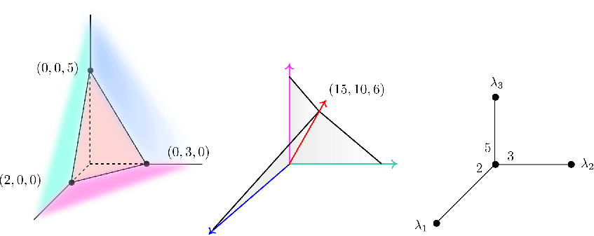
5.5.

Let $(X,0)\hookrightarrow(\mathbb{C}^{3},0)$ be the $E_{8}$ surface singularity from Subsection 2.1. As Figure 12 shows, its standard tropicalizing fan consists of the faces of the two-dimensional cones spanned by $w:=(3\cdot 5,2\cdot 5,2\cdot 3)$ and each of the coordinate weight vectors. Note that $w$ is orthogonal to the unique compact two-dimensional face of the Newton polyhedron of $f:=x^{2}+y^{3}+z^{5}$ because $f$ is $w$ -homogeneous. Note that a transversal section of the standard tropicalization of $X$ is isomorphic to its associated splice diagram. As explained in 2.36, this property holds for any splice type singularity.

The positive local tropicalization of a germ determines its local tropicalization, as the next statement confirms (see [12, Proposition 3.8] for details).

5.6.

Consider a germ $(X,0)\hookrightarrow(\mathbb{C}^{n},0)$ . The local tropicalization $\Trop X$ is the topological closure of the positive local tropicalization $\ptrop X$ inside the cone $\sigma$ .

This result was heavily used in [12] to compute local tropicalizations of splice type singularities. The same method determines the local tropicalization of edge deformations of these germs, as we discuss in Section 6.

The second main result in [12] confirms that splice type surface singularities are Newton non-degenerate. Such property characterizes the simplest germs from the toric perspective. More precisely:

5.7.

Let $(X,0)\hookrightarrow\mathbb{C}^{n}$ be a reduced germ defined by an ideal $I$ of $\mathcal{O}$ . We say that $X$ is Newton non-degenerate if for any $w\in(\mathbb{R}_{>0})^{n}$ , the $w$ -initial ideal $\operatorname{in}_{w}(I)\subset\mathbb{C}[z_{1},\ldots,z_{n}]$ defines a smooth subscheme of the algebraic torus $(\mathbb{C}^{*})^{n}$ .

5.8.

An alternative (yet equivalent) formulation of Newton non-degeneracy was proposed by Aroca, Gómez-Morales and Shabbir in [5, Definition 11.2]. They require that for each $w\in\sigma$ , the extended initial ideal $\operatorname{in}_{w}(I)\mathcal{O}\subset\mathcal{O}$ defines a smooth subscheme of the algebraic torus $(\mathbb{C}^{*})^{n}$ . Therefore, any potential singularity of the germ defined by $I$ is contained in the toric boundary.

For hypersurfaces, 5.7 coincides with the prototypical definition of Newton non-degeneracy given by Kouchnirenko [40, Definition 1.19]. It was extended to complete intersections by Khovanskii in [37, Section 2.4] (see also Oka’s book [64, page 112]). Here, we use a slight variation of it, in agreement with the setting from [12]:

5.9.

Let $(X,0)\hookrightarrow\mathbb{C}^{n}$ be a reduced germ defined by a regular sequence $(f_{1},\dots,f_{k})$ of elements of $\mathcal{O}$ . We say that this sequence is a Newton non-degenerate complete intersection presentation of $(X,0)$ if for any $w\in(\mathbb{R}_{>0})^{n}$ , the sequence of $w$ -initial forms $(\operatorname{in}_{w}(f_{1}),\dots,\operatorname{in}_{w}(f_{k}))$ defines either the empty set or a smooth complete intersection of the algebraic torus $(\mathbb{C}^{*})^{n}$ .

The difference with Khovanskii’s definition lies in the requirement of regularity of the sequence $(f_{1},\dots,f_{k})$ , i.e., it must define $(X,0)$ as a complete intersection in the standard sense. Note that if $(f_{1},\dots,f_{k})$ is a Newton non-degenerate complete intersection presentation in the sense of 5.9 and if each series $f_{i}$ is multiplied by a suitable monomial such that all those monomials contain a common variable, then the resulting sequence is no longer regular, but it nevertheless defines a Newton non-degenerate complete intersection singularity in Khovanskii’s sense.

5.9is more restrictive than 5.7. More precisely:

5.10.

Let $(f_{1},\dots,f_{k})$ be a Newton non-degenerate complete intersection presentation of a germ $(X,0)\hookrightarrow\mathbb{C}^{n}$ . Then, $(X,0)$ is Newton non-degenerate.

Proof.

Let $\mathcal{F}$ be a standard tropicalizing fan of $X$ as in 5.4. The relative interior of each cone of $\mathcal{F}$ contains at least one primitive integral weight vector. This vector is unique if, and only if, the cone is a ray. The constancy of initial ideals along relative interiors of cones of $\mathcal{F}$ ensures that it is enough to prove that for every primitive integral vector $w\in(\mathbb{R}_{>0})^{n}$ , the subscheme $Z(\operatorname{in}_{w}(I))$ of $(\mathbb{C}^{*})^{n}$ defined by $\operatorname{in}_{w}(I)$ is smooth. Here, $I$ denotes the ideal of $\mathcal{O}$ generated by $(f_{1},\dots,f_{k})$ . By hypothesis, $I$ defines the germ $X$ .

Let us fix a primitive integral vector $w\in(\mathbb{R}_{>0})^{n}$ . Consider the codimension one orbit $O_{w}$ inside the toric variety $\mathcal{X}_{\mathbb{R}_{\geq 0}w}$ . There is a natural morphism of algebraic tori $\varphi\colon(\mathbb{C}^{*})^{n}\to O_{w}$ , corresponding to the quotient morphism of the weight lattice $\mathbb{Z}^{n}$ of $(\mathbb{C}^{*})^{n}$ by the sublattice $\mathbb{Z}\,w$ . The scheme $Z(\operatorname{in}_{w}(I))$ is the preimage under $\varphi$ of the scheme-theoretic intersection $O_{w}\cap\tilde{X}$ , where $\tilde{X}$ is the strict transform of $X$ by the toric birational morphism $\mathcal{X}_{\mathbb{R}_{\geq 0}w}\to\mathbb{C}^{n}$ . Thus, it suffices to prove that $O_{w}\cap\tilde{X}$ is smooth.

As $X$ is a complete intersection germ, it is of pure dimension, say $d>0$ . Therefore, $\tilde{X}$ is also of pure-dimension $d$ , and so $O_{w}\cap\tilde{X}$ is pure of dimension $d-1$ . Since $(f_{1},\dots,f_{k})$ is a Newton non-degenerate complete intersection presentation of $(X,0)$ , we know that the strict transforms $\widetilde{Z(f_{i})}$ of the hypersurface germs $Z(f_{i})$ defined by the holomorphic germs $f_{i}$ intersect the orbit $O_{w}$ along hypersurfaces which form a normal crossings divisor in a neighborhood of their intersection. Therefore the scheme-theoretic intersection $O_{w}\cap\bigcap_{i=1}^{k}\widetilde{Z(f_{i})}$ is smooth of pure dimension $d-1$ . Since $O_{w}\cap\tilde{X}\subseteq O_{w}\cap\bigcap_{i=1}^{k}\widetilde{Z(f_{i})}$ is an inclusion of schemes of pure dimension $d-1$ , we deduce that $O_{w}\ \cap\ \tilde{X}$ is a union of irreducible components of $O_{w}\bigcap_{i=1}^{k}\widetilde{Z(f_{i})}$ . Thus, it is smooth.

We claim that, furthermore, the equality $O_{w}\cap\tilde{X}=O_{w}\cap\bigcap_{i=1}^{k}\widetilde{Z(f_{i})}$ holds. To show the missing inclusion, pick a point $p\in O_{w}\cap\bigcap_{i=1}^{k}\widetilde{Z(f_{i})}$ and let $g_{w}\in\mathcal{O}_{p}$ be a defining function of $O_{w}$ in the local ring $\mathcal{O}_{p}$ at $p$ of the complex analytic variety $\mathcal{X}_{\mathbb{R}_{\geq 0}w}$ . For every $i\in\{1,\ldots,k\}$ , we pick a defining function $\tilde{f_{i}}\in\mathcal{O}_{p}$ of the strict transform $\widetilde{Z(f_{i})}$ . Such functions exist because $\mathcal{X}_{\mathbb{R}_{\geq 0}w}$ is smooth. As $O_{w}\cap\bigcap_{i=1}^{k}\widetilde{Z(f_{i})}$ is pure of codimension $k$ in $O_{w}$ , we see that $(g_{w},\tilde{f_{1}},\dots,\tilde{f_{k}})$ is a regular sequence in the local ring $\mathcal{O}_{p}$ . Therefore, the sequence $(\tilde{f_{1}},\dots,\tilde{f_{k}},g_{w})$ is also regular. Thus, $p$ lies in the closure of the intersection $(\mathbb{C}^{*})^{n}\cap\bigcap_{i=1}^{k}\widetilde{Z(f_{i})}$ . The latter equals $(\mathbb{C}^{*})^{n}\cap\tilde{X}$ by the complete intersection hypothesis. Thus, $p\in O_{w}\cap\tilde{X}$ , as desired. ∎

The next result confirms the close interplay between Newton non-degeneracy, tropicalizing fans and toroidal varieties. It reinforces Teissier’s suggestions from [77, Section 5] to take the $\partial$ -transversality of a strict transform of a subgerm of $(\mathbb{C}^{n},0)$ by a toric modification of the ambient space as a general definition of Newton non-degeneracy for arbitrary germs in $(\mathbb{C}^{n},0)$ . More precisely:

5.11.

Let $(X,0)\hookrightarrow\mathbb{C}^{n}$ be a Newton non-degenerate germ in the sense of 5.7, and let $\mathcal{F}$ be a standard tropicalizing fan for it. Denote by $\tilde{X}$ the strict transform of $X$ by the toric birational morphism $\pi_{\mathcal{F}}\colon\mathcal{X}_{\mathcal{F}}\to\mathbb{C}^{n}$ . Then, $\tilde{X}$ is $\partial$ -transversal in the toroidal variety $(\mathcal{X}_{\mathcal{F}},\partial\mathcal{X}_{\mathcal{F}})$ in the sense of 4.1. Furthermore, the pair $(\tilde{X},\tilde{X}\cap\partial\mathcal{X}_{\mathcal{F}})$ and the morphism $(\tilde{X},\tilde{X}\cap\partial\mathcal{X}_{\mathcal{F}})\to(\mathcal{X}_{\mathcal{F}},\partial\mathcal{X}_{\mathcal{F}})$ are toroidal.

We view Theorem 5.11 as a local version of Luxton and Qu’s result [45, Theorem 1.5] regarding schön subvarieties of algebraic tori $(\mathbb{C}^{*})^{n}$ . Such subvarieties satisfy the conditions from 5.7, but in the global setting (see 4.3).

When $(X,0)$ is a Newton non-degenerate hypersurface germ and $\mathcal{F}$ is a regular fan (that is, its associated toric variety is smooth), Theorem 5.11 is a consequence of Varchenko’s results from [81, Section 10] (see also Merle’s work [49]). In turn, if $(X,0)$ is a Newton non-degenerate complete intersection and $\mathcal{F}$ is a regular fan, the statement follows from [64, Theorem III.3.4]. The last claim in the statement is obtained by combining the $\partial$ -transversality of $\tilde{X}$ with 4.4.

6. Edge deformations of splice type systems

In this section, we define the special smoothings of splice type singularities which we use to prove the Milnor fiber Conjecture (see 6.3). They depend on the choice of an internal edge of the associated splice diagram $\Gamma$ and on a triple of positive integers. The smoothings are constructed by adding scalar multiples of suitable powers of a new deformation variable $z_{0}$ to each series $F_{v,i}$ from (2.12) defining the associated splice type system $\mathcal{S}(\Gamma)$ .

Throughout, we let $\Gamma$ be a splice diagram satisfying the determinant and semigroup conditions (see Definitions 2.25 and 2.29). We fix two adjacent nodes $a,b$ of $\Gamma$ . As illustrated in Figure 4, we let $r$ be any point in the interior of $[a,b]$ and $\boxed{\widetilde{\Gamma}}$ be the rooted tree obtained by subdividing $[a,b]$ along $r$ , and fixing its root at $r$ . In order for $\widetilde{\Gamma}$ to be a splice diagram (in a slightly more general sense than we allowed in previous sections since the vertex $r$ has valency two), we must endow it with weights around $r$ . This is done via the following lemma, whose proof is a direct consequence of the positivity of the determinant of the edge $[a,b]$ :

6.1.

There exist positive coprime integers $k_{a}$ and $k_{b}$ satisfying the inequalities:

(6.1)

\frac{d_{a}}{(d_{a,b})^{2}}<\frac{k_{a}}{k_{b}}<\frac{(d_{b,a})^{2}}{d_{b}}.

In particular, the decorated diagram $\widetilde{\Gamma}$ seen on the right of Figure 13, which is obtained from $\Gamma$ by subdividing $[a,b]$ using $r$ and setting $\boxed{d_{r,a}}:=k_{a}$ , $\boxed{d_{r,b}}:=k_{b}$ , satisfies the edge determinant condition.

The weights on $\widetilde{\Gamma}$ yield a well-defined notion of linking number $\ell_{u,v}$ of any two vertices $u,v$ of $\widetilde{\Gamma}$ . In turn, we use this to write a weight vector for each node of $\widetilde{\Gamma}$ , including the root $r$ , by analogy with the construction of weight vectors for the nodes of $\Gamma$ (see (2.6)). Since $\widetilde{\Gamma}$ has the same leaves as $\Gamma$ , that is, $\partial\,\widetilde{\Gamma}=\partial\,\Gamma$ , we view the lattices $N(\partial\Gamma)$ and $M(\partial\Gamma)$ from Subsection 2.3 also as the weight lattice and lattice of exponent vectors of $\widetilde{\Gamma}$ . In particular, we set

(6.2)

\boxed{w_{r}}:=\sum_{\lambda\in\partial\,\Gamma}\ell_{r,\lambda}w_{\lambda}\in N(\partial\Gamma).

As was mentioned above, edge deformations of splice type systems depend on a triple of positive integers. Here is the precise definition:

6.2.

A triple $\boxed{(k_{a},k_{b},D)}$ of positive integers is adapted to the edge $[a,b]$ of $\Gamma$ if $k_{a}$ , $k_{b}$ satisfy the inequalities of 6.1 and $D$ is divisible by all decorations $d_{u,r}$ of $\widetilde{\Gamma}$ , when $u$ varies among the nodes of $\Gamma$ . An enrichment of $\Gamma$ relative to the edge $[a,b]$ is a choice of a triple $(k_{a},k_{b},D)$ adapted to $[a,b]$ , or equivalently, the datum of the splice diagram $\widetilde{\Gamma}$ together with the integer $D$ .

Such triples $(k_{a},k_{b},D)$ always exist, by 6.1. In order to build a deformation of the system $\mathcal{S}(\Gamma)$ for a fixed triple, we introduce a new variable $z_{0}$ (the deformation parameter) and define two extended lattices

(6.3)

\boxed{\overline{N}({\partial\Gamma})}:=\mathbb{Z}\langle w_{0}\rangle\oplus N(\partial\Gamma)\simeq\mathbb{Z}^{n+1}\hskip 20.00003pt\text{ and }\hskip 20.00003pt\boxed{\overline{M}({\partial\Gamma})}:=\mathbb{Z}\langle w_{0}^{\vee}\rangle\oplus M(\partial\Gamma)\simeq\mathbb{Z}^{n+1},

where $\boxed{w_{0}}$ and $\boxed{w_{0}^{\vee}}$ denote the basis vectors corresponding to $z_{0}$ in $\overline{N}({\partial\Gamma})$ and $\overline{M}({\partial\Gamma})$ , respectively. Analogously, for each $\lambda$ in $\partial\,\Gamma$ , we let $\boxed{\overline{w}_{\lambda}}$ be the image in $\overline{N}({\partial\Gamma})$ of the basis vector $w_{\lambda}$ from $N(\partial\Gamma)$ . Similar notation applies to each vector $\boxed{\overline{w}_{\lambda}^{\vee}}$ from $\overline{M}({\partial\Gamma})$ . We let $\boxed{\overline{N}({\partial\Gamma})_{\mathbb{R}}}:=\overline{N}({\partial\Gamma})\otimes_{\mathbb{Z}}\mathbb{R}$ and $\boxed{\overline{M}({\partial\Gamma})_{\mathbb{R}}}:=\overline{M}({\partial\Gamma})\otimes_{\mathbb{Z}}\mathbb{R}$ be the $\mathbb{R}$ -vector spaces associated to the lattices in (6.3).

The triple $(k_{a},k_{b},D)$ adapted to $[a,b]$ allows us to build new weight vectors in $\overline{N}({\partial\Gamma})$ , i.e.,

(6.4)

\boxed{\overline{w}_{u}}:=w_{0}+\frac{D\,\ell_{r,u}}{d_{u}}w_{u}\in\overline{N}({\partial\Gamma})\hskip 20.00003pt\text{ for each node }u\text{ of }\widetilde{\Gamma}.

In particular:

\overline{w}_{r}=w_{0}+Dw_{r}.

Notice that $\overline{w}_{u}\in\overline{N}({\partial\Gamma})$ since the divisibility constraint $d_{u,r}|D$ imposed on $D$ implies that $D\,\ell_{r,u}/d_{u}\in\mathbb{Z}$ . The relevance of the weight vectors $\overline{w}_{u}$ is explained in 6.4 below.

Edge deformations of splice type systems adapted to an internal edge are constructed by analogy with 2.34, as we now explain.

6.3.

Let $\mathcal{S}(\Gamma)=(F_{v,i}(\underline{z}))_{v,i}$ be a splice type system. Fix an internal edge $e=[a,b]$ of $\Gamma$ and a triple $(k_{a},k_{b},D)$ adapted to it. We view $D$ as a supplementary decoration of the splice diagram $\widetilde{\Gamma}$ .

•

An edge-deformation $\boxed{\mathcal{D}(\widetilde{\Gamma})}$ of $\mathcal{S}(\Gamma)$ associated to the previous data is a finite family of formal power series of the form:

(6.5)

\boxed{\overline{F}_{v,i}(z_{0},\underline{z})}:=F_{v,i}(\underline{z})-\boxed{c_{v,i}}\,z_{0}^{D\,\ell_{r,v}}\hskip 10.00002pt\text{for all }i\in\{1,\dots,\delta_{v}-2\}\,\text{ and each node }v\text{ of }\Gamma,

where $c_{v,i}\in\mathbb{C}^{*}$ and $F_{v,i}$ are as in (2.12).

•

An edge-deformation of the splice type singularity defined by the system $\mathcal{S}(\Gamma)$ and associated to the previous data is the subgerm at the origin of the affine space $\mathbb{C}^{n+1}$ , which is defined by an edge deformation system $\mathcal{D}(\widetilde{\Gamma})$ . The deformation parameter is the new variable $z_{0}$ .

6.4.

By analogy with 2.35 (1), we can show that our choice of exponents $D\,\ell_{r,v}$ guarantees that the polynomials $f_{v,i}(\underline{z})-c_{v,i}\,z_{0}^{D\,\ell_{r,v}}$ are $\overline{w}_{u}$ -homogeneous, where $\overline{w}_{u}$ is the weight vector from (6.4).

6.5.

As we shall see in Step (3) of Section 7, our proof of 2.41 requires an extension of 6.3 to the case where the edge $[a,b]$ is not internal, but connects a node to a leaf. We do not discuss this generalization here, to simplify the exposition.

6.5.

We let $[a,b]$ be the unique internal edge of the splice diagram $\Gamma$ from Figure 3, where $a=u$ and $b=v$ . We have multiple choices for the pairs $(k_{a},k_{b})$ satisfying $6/49<k_{a}/k_{b}<11/70$ . For an illustration, we pick $(k_{a},k_{b})=(1,7)$ . In particular, $\ell_{r,a}=42$ and $\ell_{r,b}=70$ . Thus, $w_{r}=(21,14,10,14,35)\in\mathbb{Z}^{5}$ . Moreover, $w_{a}=(147,98,60,84,210)$ and $w_{b}=(210,140,110,154,385)$ .

The integer $D$ must be divisible by both $49$ and $11$ , so we take $D=539$ . A possible edge-deformation $\mathcal{D}(\widetilde{\Gamma})$ of a strict splice-type system $\mathcal{S}(\Gamma)$ satisfying the Hamm determinant condition of 2.34 is

(6.6)

\begin{cases}\overline{f}_{a,1}:=\;\;\;\,z_{1}^{2}\;\;\;-\;\;\;2\;z_{2}^{3}\;+\;\;\;z_{4}\,z_{5}\;\;\;+\;\;\;z_{0}^{22638},\\ \overline{f}_{b,1}:=\;\;\;\;z_{1}z_{2}^{4}+z_{3}^{7}+\;\;z_{4}^{5}\,-\;2155\;z_{5}^{2}+z_{0}^{37730},\\ \overline{f}_{b,2}:=33\,z_{1}z_{2}^{4}+z_{3}^{7}+2\,z_{4}^{5}-\;2123\,z_{5}^{2}-z_{0}^{37730}.\end{cases}

In particular, the three relevant extended weight vectors are $\overline{w}_{r}=(1,79233,52822,32340,45276,113190)$ , $\overline{w}_{a}=(1,11319,7546,4620,6468,16170)$ and $\overline{w}_{b}=(1,10290,6860,5390,7546,18865)$ .

In order for the germ defined by $\mathcal{D}(\widetilde{\Gamma})$ to have a prescribed local tropicalization, we must impose further genericity constraints on the coefficients $c_{v,i}$ . To this end, given any $w\in(\mathbb{R}_{>0})^{n+1}\subset\overline{N}({\partial\Gamma})_{\mathbb{R}}$ we consider the map

(6.7)

\boxed{F_{w}}\colon\mathbb{C}^{n}\to\mathbb{C}^{n-2}\hskip 20.00003ptF_{w}(\underline{z})=(\operatorname{in}_{w}(F_{v,i})(\underline{z}))_{v,i}

whose entries are determined by the set of initial forms of all equations $F_{v,i}$ defining the system $\mathcal{S}(\Gamma)$ . When restricted to codimension two coordinate subspaces of $\mathbb{C}^{n}$ , the map $F_{w}$ satisfies the following key property:

6.6.

For each $w\in\Trop X$ and any pair of distinct leaves $\lambda,\mu$ of $\Gamma$ , the restriction map $\boxed{F_{w,\lambda,\mu}}\colon\mathbb{C}^{n-2}\to\mathbb{C}^{n-2}$ to the coordinate subspace $Z(z_{\lambda},z_{\mu})$ of $\mathbb{C}^{n}$ is generically finite, hence dominant.

This result allows us to specify explicit genericity conditions on the coefficients $c_{v,i}$ from (6.5) that are suitable for proving 2.41. Under such genericity conditions, we can verify that the vanishing sets of both $\mathcal{S}(\Gamma)$ and the edge-deformation $\mathcal{D}(\widetilde{\Gamma})$ have similar behavior. More precisely,

6.7.

Assume that $(c_{v,i})_{v,i}$ are generic and let $\mathcal{Y}(\widetilde{\Gamma})$ be the vanishing set of the edge-deformation $\mathcal{D}(\widetilde{\Gamma})$ in $\mathbb{C}^{n+1}$ . Then,

(1)

the germ $(\mathcal{Y}(\widetilde{\Gamma}),0)$ is a three-dimensional reduced and irreducible isolated complete intersection singularity not contained in the toric boundary of $\mathbb{C}^{n+1}$ ;
(2)

the series defining the edge-deformation $\mathcal{D}(\widetilde{\Gamma})$ determine a Newton non-degenerate complete intersection presentation of its vanishing set $\mathcal{Y}(\widetilde{\Gamma})$ ;
(3)

the local tropicalization $\Trop\mathcal{Y}(\widetilde{\Gamma})\subset(\mathbb{R}_{\geq 0})^{n+1}$ is independent of $\mathcal{D}(\widetilde{\Gamma})$ and its coarsest fan structure is a standard tropicalizing fan for $\mathcal{Y}(\widetilde{\Gamma})$ .

6.8.

The description of the top-dimensional cones of the standard tropicalization fan of $\mathcal{Y}(\widetilde{\Gamma})$ mentioned above is a bit more cumbersome than for the splice type system $\mathcal{S}(\Gamma)$ discussed in 2.36. The explicit construction of this fan is used in Step (8) of Section 7 as well as in the proof of Theorem 6.7 (2) under explicit genericity conditions. The rays of $\Trop\mathcal{Y}(\widetilde{\Gamma})$ are easy to list: they are generated by the weight vectors $\overline{w}_{u}$ indexed by all vertices $u$ of the enriched splice diagram $\widetilde{\Gamma}$ plus one more ray corresponding to the deformation variable. The fan is non-simplicial and its unique non-simplicial top-dimensional cone is spanned by $w_{0},w_{a},w_{b}$ and $w_{r}$ . The presence of this last cone reveals the product structure of the central component of the Milnor fiber of the germ defined by $\mathcal{S}(\Gamma)$ (see Step (27)).

7. Proof outline of the Milnor fiber conjecture

In this section, we outline our proof of Neumann and Wahl’s Milnor fiber conjecture (see 2.41) through a sequence of 28 steps. Each step has a title, describing it briefly. The main statements proved at each step are written with boldface characters. The first four steps set up the deformations and smoothings of various splice type systems. The tropical techniques are used in Steps (5) through (12), whereas logarithmic geometry features from Step (13) onwards. This decomposition into steps is much more detailed than the decomposition into stages explained in Section 1. The correspondence between them is as follows: Stage 1 corresponds to Steps (1) and (2); Stage 2 to Steps (3) and (4); Stage 3 to Steps (5), (6) and (9); Stage 4 to Steps (7) and (11); Stage 5 to Steps (13), (14), (15) and (19); Stage 6 to Steps (8), (10), (12), (16), (17), (18), (20), (21), (22), (23), (24) and (25); Stage 7 to the remaining Steps (26), (27) and (28).

We start from a splice diagram $\Gamma$ (see 2.22) with $n$ leaves and at least two nodes, which satisfies the edge determinant condition of 2.25 and the semigroup condition of 2.29. We let $\boxed{(X,0)}\hookrightarrow(\mathbb{C}^{n},0)$ be a splice type singularity defined by a splice type system $\boxed{\mathcal{S}(\Gamma)}$ as in 2.34. Fixing an internal edge $[a,b]$ of $\Gamma$ determines a partition of $\mathcal{S}(\Gamma)$ into two systems: an $a$ -side system $\boxed{\mathcal{S}_{a}(\Gamma)}$ , combining the series associated to all the nodes seen from $b$ in the direction of $a$ , and a $b$ -side system $\boxed{\mathcal{S}_{b}(\Gamma)}$ involving the series associated to all the nodes of $\Gamma$ seen from $a$ in the direction of $b$ .

(1)

We enrich the splice diagram $\Gamma$ .

We subdivide the splice diagram $\Gamma$ using an interior point $\boxed{r}$ of the edge $[a,b]$ and we let $\boxed{\widetilde{\Gamma}}$ be the resulting tree, rooted at the vertex $r$ . We choose a triple $\boxed{(k_{a},k_{b},D)}$ adapted to $[a,b]$ in the sense of 6.2 and we view $\widetilde{\Gamma}$ as a splice diagram (with weights $d_{r,a}=k_{a}$ and $d_{r,b}=k_{b}$ ) enriched by $D$ .

(2)

We perform an edge deformation of the starting splice type system.

We consider an edge deformation $\boxed{\mathcal{D}(\widetilde{\Gamma})}$ of the system $\mathcal{S}(\Gamma)$ in the sense of 6.3 with deformation parameter $\boxed{z_{0}}$ . We assume that the coefficients $(c_{v,i})_{v,i}\in(\mathbb{C}^{*})^{n-2}$ satisfy the genericity constraints mentioned in Section 6. We write $\mathcal{D}(\widetilde{\Gamma})$ as the disjoint union of a deformed $a$ -side system $\boxed{\mathcal{D}(\widetilde{\Gamma})_{a}}$ and a deformed $b$ -side system $\boxed{\mathcal{D}(\widetilde{\Gamma})_{b}}$ .

We let $\boxed{(Y,0)}\hookrightarrow\mathbb{C}^{n+1}$ be the singularity defined by $\mathcal{D}(\widetilde{\Gamma})$ and denote by $\boxed{f}\colon Y\to\mathbb{C}$ the restriction of the linear form $z_{0}\colon\mathbb{C}^{n+1}\to\mathbb{C}$ to $Y$ . We prove that $f$ is a smoothing of the splice type singularity $(X,0)$ and incorporate it into the following commutative diagram:

(7.1)

(3)

We define the notion of an $a$ -side morphism associated to the given edge deformation.

Let $u$ be a node of the rooted tree $\Gamma_{a}$ , seen as a subtree of $\widetilde{\Gamma}$ in Figure 4. We prove that the $w_{u}$ -initial forms of the series of the system $\mathcal{D}(\widetilde{\Gamma})_{b}$ are independent of the choice of $u$ . We let $\boxed{\operatorname{in}_{a}(\mathcal{D}(\widetilde{\Gamma})_{b})}$ be the system determined by the vanishing of these $(n_{b}-1)$ initial forms.

We prove that the system $\operatorname{in}_{a}(\mathcal{D}(\widetilde{\Gamma})_{b})$ defines a torus-translated toric subvariety of $\mathbb{C}^{n+1}$ of dimension $n_{a}+1$ . Furthermore, this subvariety admits a normalization morphism

(7.2) $\boxed{\varphi_{a}}\colon\mathbb{C}^{n_{a}+1}\to\mathbb{C}^{n+1},$

where $\varphi_{a}$ is a monomial map (i.e., a torus-translated toric morphism). Moreover, we have

(7.3) $\varphi_{a}^{*}z_{0}=x_{0},$

where $\boxed{x_{0}}$ is one of the variables of $\mathbb{C}^{n_{a}+1}$ . We call $\varphi_{a}$ the $a$ -side morphism.

(4)

We define an $a$ -side deformation by a coordinate change of $\mathbb{C}^{n_{a}+1}$ using the $a$ -side morphism $\varphi_{a}$
from (7.2).

We define a system $\boxed{\mathcal{D}(\Gamma_{a})}$ by pulling back the system $\mathcal{D}(\widetilde{\Gamma})_{a}$ via the $a$ -side morphism $\varphi_{a}$ . We let $\boxed{(Y_{a},0)}\hookrightarrow\mathbb{C}^{n_{a}+1}$ be the singularity defined by the system $\mathcal{D}(\Gamma_{a})$ . Analogously, we let $\boxed{\mathcal{S}(\Gamma_{a})}$ be the pullback of the system $\mathcal{S}(\Gamma)$ via $\varphi_{a}$ . By construction, $\mathcal{S}(\Gamma_{a})$ does not involve the variable $x_{0}$ . We identify the coordinate hyperplane $Z(x_{0})$ of $\mathbb{C}^{n_{a}+1}$ with $\mathbb{C}^{n_{a}}$ , and denote by $\boxed{(X_{a},0)}\hookrightarrow(\mathbb{C}^{n_{a}},0)$ the singularity defined by the system $\mathcal{S}(\Gamma_{a})$ .

We show that $\mathcal{S}(\Gamma_{a})$ is a splice type system with splice diagram $\Gamma_{a}$ and that the system $\mathcal{D}(\Gamma_{a})$ is an edge deformation of $\mathcal{S}(\Gamma_{a})$ associated to the edge $[a,r_{a}]$ , with deformation variable $x_{0}$ (see Figure 4). Notice that this last point requires us to extend our definition of edge deformations to non-internal edges of splice diagrams. As a consequence, the restriction of the linear map $x_{0}\colon\mathbb{C}^{n_{a}+1}\to\mathbb{C}$ to $(Y_{a},0)$ is a smoothing of $(X_{a},0)$ . We denote it by $f_{a}\colon(Y_{a},0)\to\mathbb{C}$ . The above data fit into the following commutative diagram analogous to (7.1):

(7.4)

As expected, we perform analogous constructions on the $b$ -side, denoting by $\boxed{y_{0}}$ the corresponding deformation variable and by $\boxed{\varphi_{b}}$ the $b$ -side morphism. Since the construction is symmetric in $a$ and $b$ , we restrict our exposition to matters concerning only the $a$ -side.

(5)

We build a standard tropicalizing fan for $(X,0)$ and prove that $(X,0)$ is Newton non-degenerate.

We construct a standard tropicalizing fan $\boxed{\mathcal{F}_{X}}$ for the embedding $(X,0)\hookrightarrow\mathbb{C}^{n}$ in the sense of 5.4 and use it to prove that the system $\mathcal{S}(\Gamma)$ is a Newton non-degenerate complete intersection presentation of $(X,0)$ , in the sense of 5.9. Complete proofs for these assertions can be found in [12].

We prove that the fan $\mathcal{F}_{X}$ is a cone over a suitable embedding of the splice diagram $\Gamma$ in the standard simplex $\Delta_{n-1}\subset\mathbb{R}^{n}$ (see [12, Theorem 1.2]). Its rays are in bijection with the vertices of $\Gamma$ and its two-dimensional cones are spanned by pairs of rays corresponding to adjacent vertices of $\Gamma$ . Thus, the splice diagram appears as a transversal section of the local tropicalization of $(X,0)\hookrightarrow\mathbb{C}^{n}$ . This gives the first tropical interpretation of splice diagrams, in the case when both the determinant and the semigroup conditions are satisfied.
(6)

We build a standard tropicalizing fan for $(Y,0)$ and prove that this germ is Newton non-degenerate.

Using the results of Step (5), we describe a standard tropicalizing fan $\boxed{\mathcal{F}}$ for the embedding $(Y,0)\hookrightarrow\mathbb{C}^{n+1}$ and prove that the system $\mathcal{D}(\widetilde{\Gamma})$ is a Newton non-degenerate complete intersection presentation of $(Y,0)$ . The genericity conditions on $\mathcal{D}(\widetilde{\Gamma})$ are essential to determine $\mathcal{F}$ , as discussed in Theorem 6.7. A partial description of $\mathcal{F}$ is given in 6.8. Our proof uses results and techniques from [12]. In particular, we show that the $2$ -dimensional fan $\mathcal{F}_{X}$ introduced at Step (5) is the union of strata at infinity of $\mathcal{F}$ corresponding to the vanishing of the deformation parameter $z_{0}$ (see 5.3).

(7)

We describe a quasi-toroidalization of the smoothing $f$ of $(X,0)$ from Step (2).

We let $\boxed{\pi_{\mathcal{F}}}\colon\mathcal{X}_{\mathcal{F}}\to\mathbb{C}^{n+1}$ be the toric birational morphism defined by the fan $\mathcal{F}$ of Step (6) and we denote by $\boxed{\pi}\colon\tilde{Y}\to Y$ the restriction of $\pi_{\mathcal{F}}$ to the strict transform $\tilde{Y}$ of $Y$ by $\pi_{\mathcal{F}}$ . Since $\mathcal{F}$ is a tropicalizing fan for $(Y,0)\hookrightarrow\mathbb{C}^{n+1}$ , 5.1 ensures that $\phi$ is a modification, unlike the case of the non-proper toric birational map $\pi_{\mathcal{F}}$ . These data fit into the commutative diagram

Using Theorem 5.11, we prove that $\pi$ is a quasi-toroidalization of $f$ (see 4.7). This statement follows from the fact that the deformed system $\mathcal{D}(\widetilde{\Gamma})$ is a Newton non-degenerate complete intersection presentation of $(Y,0)$ , as discussed in Step (6).

(8)

We prove that the dual complex of the exceptional divisor of $\pi$ is a subtree of $\widetilde{\Gamma}$ .

The structure of the fan $\mathcal{F}$ introduced in Step (6) allows to prove that the dual complex of the (compact) exceptional divisor $\partial_{0}\tilde{Y}$ of $\pi\colon\tilde{Y}\to Y$ is canonically isomorphic to the unique connected subtree of $\widetilde{\Gamma}$ with vertex set equal to the set of nodes of $\tilde{\Gamma}$ . This induces a decomposition of $\partial_{0}\tilde{Y}$ as a sum of three reduced divisors, namely:

(7.5) $\partial_{0}\tilde{Y}=\boxed{\partial_{a}\tilde{Y}}+\boxed{\partial_{r}\tilde{Y}}+\boxed{\partial_{b}\tilde{Y}}.$

Here, $\partial_{a}\tilde{Y}$ is the sum of irreducible components of $\partial_{0}\tilde{Y}$ corresponding to the nodes of $\Gamma_{a}$ and similarly for $b$ . In turn, $\partial_{r}\tilde{Y}$ is an irreducible variety corresponding to the root $r$ of $\widetilde{\Gamma}$ .
(9)

We perform the $a$ -side analog of Step (6).

We determine a standard tropicalizing fan $\mathcal{F}_{a}$ for $(Y_{a},0)\hookrightarrow\mathbb{C}^{n_{a}+1}$ and we use it to prove that the system $\mathcal{D}(\Gamma_{a})$ introduced in Step (4) is a Newton non-degenerate complete intersection presentation of $(Y_{a},0)$ .

The rays of the fan $\mathcal{F}_{a}$ correspond bijectively to the vertices of the rooted tree $\Gamma_{a}$ , excepted for a single ray, which is the coordinate ray associated to the deformation variable $x_{0}$ . The cones spanned by pairs of rays corresponding to adjacent vertices of $\Gamma_{a}$ belong to the set of two-dimensional cones of $\mathcal{F}_{a}$ . There are extra two-dimensional cones of $\mathcal{F}_{a}$ not included in this list. The three-dimensional cones are spanned by some triples of rays of $\mathcal{F}_{a}$ .
(10)

We compare objects associated to $X$ and their counterparts on the $a$ -side singularity $X_{a}$ .

Consider the torus-translated toric morphism $\varphi_{a}\colon\mathbb{C}^{n_{a}+1}\to\mathbb{C}^{n+1}$ introduced in Step (3). We prove that the associated linear map $\phi_{a}\colon N(\Gamma_{a})_{\mathbb{R}}\to N(\Gamma)_{\mathbb{R}}$ between weight spaces almost embeds the fan $\mathcal{F}_{a}$ inside the fan $\mathcal{F}$ . More precisely, it is an embedding when restricted to the subfan of $\mathcal{F}_{a}$ spanned by the rays associated to any vertex of $\Gamma_{a}$ other than the root $r_{a}$ . Furthermore, the ray $\boxed{l_{r}}$ of $\mathcal{F}$ associated to the root $r$ of $\widetilde{\Gamma}$ lies in the relative interior of the image under $\phi_{a}$ of the two-dimensional cone of $\mathcal{F}_{a}$ spanned by the rays corresponding to the vertices $a$ and $r_{a}$ of $\Gamma_{a}$ .

We write $\boxed{l_{a,r}}:=\phi_{a}^{-1}(\{l_{r}\})\subseteq N(\Gamma_{a})_{\mathbb{R}}$ and let $\boxed{\mathcal{F}_{a,r}}$ be the fan obtained by performing the stellar subdivision of $\mathcal{F}_{a}$ along $l_{a,r}$ . Since it refines the standard tropicalizing fan $\mathcal{F}_{a}$ for $(Y_{a},0)\hookrightarrow\mathbb{C}^{n_{a}+1}$ from Step (9), $\mathcal{F}_{a,r}$ is also a standard tropicalizing fan for $Y_{a}$ .

(11)

We perform the $a$ -side analog of Step (7).

Let $\boxed{\pi_{a,r}}\colon\tilde{Y}_{a}\to Y_{a}$ be the restriction of the toric birational morphism $\pi_{\mathcal{F}_{a,r}}\colon\mathcal{X}_{\mathcal{F}_{a,r}}\to\mathbb{C}^{n_{a}+1}$ to the strict transform $\boxed{\tilde{Y}_{a}}$ of $Y_{a}$ by $\pi_{\mathcal{F}_{a,r}}$ . As $\mathcal{F}_{a,r}$ is a tropicalizing fan for $(Y_{a},0)\hookrightarrow\mathbb{C}^{n+1}$ by Step (10), the morphism $\pi_{a,r}$ is a modification. This determines the commutative diagram

Since the deformed system $\mathcal{D}(\Gamma_{a})$ is a Newton non-degenerate complete intersection presentation of $(Y_{a},0)$ by Step (9), Theorem 5.11 confirms that $\pi_{a,r}$ is a quasi-toroidalization of $f_{a}$ .

(12)

We continue comparing objects associated to $X$ with their counterparts on the $a$ -side singularity $X_{a}$ .

We let $\boxed{\mathcal{F}_{a,r}^{-}}$ be the subfan of $\mathcal{F}_{a,r}$ consisting of all cones not containing the ray associated to the root $r_{a}$ of $\Gamma_{a}$ . By construction, the linear map $\phi_{a}$ from Step (10) embeds $\mathcal{F}_{a,r}^{-}$ into $\mathcal{F}$ . Therefore, we can lift $\varphi_{a}$ to a torus-translated morphism $\boxed{\Phi_{a}}\colon\mathcal{X}_{\mathcal{F}_{a,r}^{-}}\to\mathcal{X}_{\mathcal{F}}$ fitting into the following commutative diagram

with the additional property that the morphism $\Phi_{a}$ is a toric embedding, that is, a toric morphism which is an embedding of algebraic varieties.

(13)

We build the log special fiber of a log enhancement of the lifting $\tilde{f}=f\circ\pi$ , where $\pi$ is the quasi-
toroidalization of $f$ from Step (7).

Following the discussion preceding 4.52, we choose a Milnor tube representative $f\colon Y\to\mathbb{D}$ of the smoothing $f$ and we consider its lift $\boxed{\tilde{f}}:=f\circ\pi\colon\tilde{Y}\to\mathbb{D}$ to the modified space $\tilde{Y}$ introduced in Step (7). Recall that $\pi$ is a quasi-toroidalization of $f$ . We consider the log enhancement of $f$ relative to the divisors $Z(\tilde{f})$ and $\{0\}$ in the sense of 4.32, i.e.,

\boxed{\tilde{f}^{\dagger}}\colon\tilde{Y}^{\dagger}\to\mathbb{D}^{\dagger},

where $\boxed{\tilde{Y}^{\dagger}}:=(Y,\mathcal{O}^{\star}_{\tilde{Y}}(-Z(\tilde{f})))$ and $\boxed{\mathbb{D}^{\dagger}}:=(\mathbb{D},\mathcal{O}^{\star}_{\mathbb{D}}(-\{0\}))$ are log complex spaces. At the level of sheaves of monoids, $\tilde{f}^{\dagger}$ is simply the pullback of functions by $\tilde{f}$ .

Consider now the log special fiber of the morphism $\tilde{f}^{\dagger}$

(7.6)

\boxed{(\tilde{f}_{0})^{\dagger}}\colon\boxed{Z(\tilde{f})^{\dagger}}\to\boxed{0^{\dagger}},

obtained by restricting the log structures of the source and target spaces to the special fiber of $\tilde{f}$ and to $\{0\}\hookrightarrow\mathbb{D}$ , respectively (see 4.25). The construction yields a commutative diagram in the log category:

(7.7)

Note that both horizontal arrows are strict, in the sense of 4.28.

(14)

We show that the rounding of the log enhancement of $\tilde{f}$ is a representative of the Milnor fibration
of $f$ .

Consider the rounding of the diagram (7.7) in the sense of 4.42:

(7.8)

Note that $0^{\dagger}_{\log}$ is a circle, identified canonically with complex numbers of modulus one through the use of polar coordinates. As both horizontal arrows in (7.7) are strict, 4.48 implies that the diagram (7.8) is cartesian in the topological category.

Using 4.51, which is a direct consequence of Nakayama and Ogus’ local triviality theorem (see Theorem 4.49), we conclude that the left vertical arrow of (7.8) is a representative of the circular Milnor fibration of $f$ .

(15)

We build a new representative of the Milnor fibration of $f$ by removing a collar neighborhood of the
boundary of the total space of the fibration of Step (14).

We consider the rounding map of the complex log space $Z(\tilde{f})^{\dagger}$ :

\tau_{Z(\tilde{f})^{\dagger}}\colon Z(\tilde{f})^{\dagger}_{\log}\to Z(\tilde{f}).

We build a new representative of the circular Milnor fibration of $f$ using the restriction

(7.9)

(\tilde{f_{0}})^{\dagger}_{\log}|_{\tau_{Z(\tilde{f})^{\dagger}}^{-1}(\partial_{0}\tilde{Y})}\colon\tau_{Z(\tilde{f})^{\dagger}}^{-1}(\partial_{0}\tilde{Y})\to 0^{\dagger}_{\log}

of the leftmost vertical arrow from (7.8) to the preimage $\tau_{Z(\tilde{f})^{\dagger}}^{-1}(\partial_{0}\tilde{Y})$ of the exceptional divisor $\partial_{0}\tilde{Y}=\pi^{-1}(0)$ of $\pi$ under the rounding map $\tau_{Z(\tilde{f})^{\dagger}}$ . Note that the divisor $\partial_{0}\tilde{Y}$ already featured in Step (7) and that the complement of $\tau_{Z(\tilde{f})^{\dagger}}^{-1}(\partial_{0}\tilde{Y})$ in $Z(\tilde{f})^{\dagger}_{\log}$ is a collar neighborhood of the topological boundary of $Z(\tilde{f})^{\dagger}_{\log}$ . The latter fact is crucial to prove the claim.

(16)

We prove that rounding yields a canonical decomposition of the source of the Milnor fibration of $f$ .

The decomposition (7.5) induces the following decomposition of the source space of the representative (7.9) of the circular Milnor fibration of $f$ :

\tau_{Z(\tilde{f})^{\dagger}}^{-1}(\partial_{0}\tilde{Y})=\tau_{Z(\tilde{f})^{\dagger}}^{-1}(\partial_{a}\tilde{Y})\>\>\cup\>\>\tau_{Z(\tilde{f})^{\dagger}}^{-1}(\partial_{r}\tilde{Y})\>\>\cup\>\>\tau_{Z(\tilde{f})^{\dagger}}^{-1}(\partial_{b}\tilde{Y}).

We prove that when restricted to the three parts of this decomposition, the rounding morphism $(\tilde{f}_{0})^{\dagger}_{\log}$ is isomorphic to the roundings of the log morphisms

(7.10)

(\partial_{a}\tilde{Y},\mathcal{O}^{\star}_{\tilde{Y}|\partial_{a}\tilde{Y}}(-Z(\tilde{f})))\to 0^{\dagger},\hskip 10.00002pt(\partial_{r}\tilde{Y},\mathcal{O}^{\star}_{\tilde{Y}|\partial_{r}\tilde{Y}}(-Z(\tilde{f})))\to 0^{\dagger}\;\text{ and }\;(\partial_{b}\tilde{Y},\mathcal{O}^{\star}_{\tilde{Y}|\partial_{b}\tilde{Y}}(-Z(\tilde{f})))\to 0^{\dagger}

obtained by restricting the log special fiber (7.6) to the subdivisors $\partial_{a}\tilde{Y},\partial_{r}\tilde{Y}$ and $\partial_{b}\tilde{Y}$ of $Z(\tilde{f})$ , respectively.

(17)

We prove that the three log morphisms from (7.10) can be obtained by restrictions from the ambient
toric varieties.

Using the functoriality of restriction of log structures, we prove that the log morphisms of (7.10) are isomorphic to the log morphisms

(7.11)

(\partial_{a}\tilde{Y},\mathcal{O}^{\star}_{\mathcal{X}_{\mathcal{F}}|\partial_{a}\tilde{Y}}(-Z(\tilde{z_{0}})))\to 0^{\dagger},\;\;(\partial_{r}\tilde{Y},\mathcal{O}^{\star}_{\mathcal{X}_{\mathcal{F}}|\partial_{r}\tilde{Y}}(-Z(\tilde{z_{0}})))\to 0^{\dagger}\text{ and }(\partial_{b}\tilde{Y},\mathcal{O}^{\star}_{\mathcal{X}_{\mathcal{F}}|\partial_{b}\tilde{Y}}(-Z(\tilde{z_{0}})))\to 0^{\dagger}

obtained by restricting the logarithmic enhancement $\tilde{z_{0}}^{\dagger}\colon\mathcal{X}_{\mathcal{F}}^{\dagger}\to\mathbb{C}^{\dagger}$ of the linear map $\tilde{z_{0}}\colon\mathcal{X}_{\mathcal{F}}\to\mathbb{C}$ to the subdivisors $\partial_{a}\tilde{Y},\partial_{r}\tilde{Y}$ and $\partial_{b}\tilde{Y}$ of $Z(\tilde{f})$ , respectively. Here, $\boxed{\mathcal{X}_{\mathcal{F}}^{\dagger}}$ denotes the divisorial complex log space $(\mathcal{X}_{\mathcal{F}},\mathcal{O}_{\mathcal{X}_{\mathcal{F}}}^{\star}(-Z(\tilde{z_{0}})))$ .

(18)

We describe the $a$ -side parts of the Milnor fibers of $f$ .

Using the results of Steps (13) through (17), we deduce that the fibers of the rounding

(\partial_{a}\tilde{Y},\mathcal{O}^{\star}_{\mathcal{X}_{\mathcal{F}}|\partial_{a}\tilde{Y}}(-Z(\tilde{z_{0}})))_{\log}\to 0^{\dagger}_{\log}

of the first arrow of (7.11) are homeomorphic to the parts of the fibers of the representative $(\tilde{f}_{0})^{\dagger}_{\log}\colon Z(\tilde{f})^{\dagger}_{\log}\to 0^{\dagger}_{\log}$ of the circular Milnor fibration of $f$ contained inside $\tau_{Z(\tilde{f})^{\dagger}}^{-1}(\partial_{a}\tilde{Y})$ .

(19)

We perform an $a$ -side analog of Steps (13), (14) and (15).

We choose a Milnor tube representative $f_{a}\colon Y_{a}\to\mathbb{D}$ of the smoothing $f_{a}$ of $(X_{a},0)$ appearing in diagram (7.4) and we consider its lift $\boxed{\tilde{f}_{a}}:=f_{a}\circ\pi_{a,r}\colon\tilde{Y}_{a}\to\mathbb{D}$ to the modified space $\tilde{Y}_{a}$ introduced in Step (11). Recall that $\pi_{a,r}$ is a quasi-toroidalization of $f_{a}$ .

Consider the log enhancement of $f_{a}$ relative to the divisors $Z(\tilde{f}_{a})$ and $0$ :

\boxed{\tilde{f}^{\dagger}_{a}}\colon\boxed{\tilde{Y}^{\dagger}_{a}}\to\mathbb{D}^{\dagger}.

In turn, we build the log special fiber of the morphism $\tilde{f}^{\dagger}_{a}$ and its rounding, i.e.

(7.12)

(\tilde{f}_{a,0})^{\dagger}\colon Z(\tilde{f}_{a})^{\dagger}\to 0^{\dagger}\hskip 20.00003pt\text{ and }\hskip 20.00003pt(\tilde{f}_{a,0})^{\dagger}_{\log}\colon Z(\tilde{f}_{a})^{\dagger}_{\log}\to 0^{\dagger}_{\log}.

Let $\tau_{Z(\tilde{f}_{a})^{\dagger}}\colon Z(\tilde{f}_{a})^{\dagger}_{\log}\to Z(\tilde{f}_{a})$ be the rounding map of the complex log space $Z(\tilde{f}_{a})^{\dagger}$ . We show that the restriction of the rounding morphism $(\tilde{f}_{a,0})^{\dagger}_{\log}$ from (7.12) to the preimage $\tau_{Z(\tilde{f}_{a})^{\dagger}}^{-1}(\partial_{0}\tilde{Y}_{a})$ of the exceptional divisor $\boxed{\partial_{0}\tilde{Y}_{a}}:=\pi_{a,r}^{-1}(0)$ of $\pi_{a,r}$ under the rounding map $\tau_{Z(\tilde{f}_{a})^{\dagger}}$ gives a representative of the circular Milnor fibration of $f_{a}$ .

(20)

We perform an $a$ -side analog of Step (16).

We prove that when restricted to $\tau_{Z(\tilde{f}_{a})^{\dagger}}^{-1}(\partial_{0}\tilde{Y}_{a})$ , the rounding morphism $(\tilde{f}_{a,0})^{\dagger}_{\log}$ from (7.12) is isomorphic to the rounding of the log morphism

$(\partial_{0}\tilde{Y}_{a},\mathcal{O}^{\star}_{\tilde{Y}_{a}|\partial_{0}\tilde{Y}_{a}}(-Z(\tilde{f}_{a})))\to 0^{\dagger}$

obtained by restricting the log special fiber map $(\tilde{f}_{a,0})^{\dagger}$ from (7.12) to the subdivisor $\partial_{0}\tilde{Y}_{a}$ of $Z(\tilde{f}_{a})$ .

(21)

We perform an $a$ -side analog of Step (17).

Recall that the variable $x_{0}$ of $\mathbb{C}^{n_{a}+1}$ , introduced in Step (3), denotes the deformation variable of the $a$ -side system $\mathcal{D}(\Gamma_{a})$ of Step (4). Consider the tropicalizing fan $\mathcal{F}_{a,r}$ for $Y_{a}$ introduced in Step (10). Let $\boxed{\mathcal{X}_{\mathcal{F}_{a,r}}^{\dagger}}$ denote the divisorial complex log space $(\mathcal{X}_{\mathcal{F}_{a,r}},\mathcal{O}_{\mathcal{X}_{\mathcal{F}_{a,r}}}^{\star}(-Z(\tilde{x}_{0})))$ and let

\boxed{\tilde{x_{0}}^{\dagger}}\colon\mathcal{X}_{\mathcal{F}_{a,r}}^{\dagger}\to\mathbb{D}^{\dagger}

be the logarithmic enhancement of $\tilde{x_{0}}$ relative to the divisors $Z(\tilde{x}_{0})$ and $0$ . We prove that the log morphism (20) is isomorphic to the log morphism

(7.13)

\tilde{x_{0}}^{\dagger}|_{\partial_{0}\tilde{Y}_{a}}\colon(\partial_{0}\tilde{Y}_{a},\mathcal{O}^{\star}_{\mathcal{X}_{\mathcal{F}_{a,r}}|\partial_{0}\tilde{Y}_{a}}(-Z(\tilde{x}_{0})))\to 0^{\dagger}

obtained by restricting $\tilde{x_{0}}^{\dagger}$ to the subdivisor $\partial_{0}\tilde{Y}_{a}$ of $Z(\tilde{f}_{a})$ .

(22)

We perform an $a$ -side analog of Step (18).

Using the results of Steps (19), (20) and (21), we deduce that the fibers of the rounding

(\partial_{0}\tilde{Y}_{a},\mathcal{O}^{\star}_{\mathcal{X}_{\mathcal{F}_{a,r}}|\partial_{0}\tilde{Y}_{a}}(-Z(\tilde{x}_{0})))_{\log}\to 0^{\dagger}_{\log}

of the log morphism (7.13) are homeomorphic to the fibers of the representative

(\tilde{f}_{a,0})^{\dagger}_{\log}\colon\tau_{Z(\tilde{f}_{a})^{\dagger}}^{-1}(\partial_{0}\tilde{Y}_{a})\to 0^{\dagger}_{\log}

of the circular Milnor fibration of the smoothing $f_{a}$ of $X_{a}$ .

(23)

We compare the objects associated to the starting singularity $X$ and to the $a$ -side singularity $X_{a}$ , as
a sequel to Steps (10) and (12), by constructing a natural map from an $a$ -side log morphism to a
log morphism associated with the initial smoothing.

Recall the fan $\mathcal{F}_{a,r}^{-}$ and the torus-translated toric morphism $\Phi_{a}\colon\mathcal{X}_{\mathcal{F}_{a,r}^{-}}\to\mathcal{X}_{\mathcal{F}}$ introduced in Step (12). The relation (7.3) ensures that the following triangle of torus-translated toric morphisms commutes:

\lx@xy@svg{\hbox{\raise 2.55554pt\hbox{\kern 14.53798pt\hbox{\ignorespaces\ignorespaces\ignorespaces\hbox{\vtop{\halign{\entry@#!@&&\entry@@#!@\cr&&\cr&&\crcr}}}\ignorespaces{\hbox{\kern-14.53798pt\raise 0.0pt\hbox{\hbox{\kern 0.0pt\raise 0.0pt\hbox{\hbox{\kern 3.0pt\raise-2.55554pt\hbox{$\textstyle{\mathcal{X}_{\mathcal{F}_{a,r}^{-}}\ignorespaces\ignorespaces\ignorespaces\ignorespaces\ignorespaces\ignorespaces\ignorespaces\ignorespaces}$}}}}}}}\ignorespaces\ignorespaces\ignorespaces\ignorespaces{}{\hbox{\lx@xy@droprule}}\ignorespaces\ignorespaces\ignorespaces{\hbox{\kern 34.62979pt\raise 5.89168pt\hbox{{}\hbox{\kern 0.0pt\raise 0.0pt\hbox{\hbox{\kern 3.0pt\hbox{\hbox{\kern 0.0pt\raise-1.89168pt\hbox{$\scriptstyle{\Phi_{a}}$}}}\kern 3.0pt}}}}}}\ignorespaces{\hbox{\kern 75.76021pt\raise 0.0pt\hbox{\hbox{\kern 0.0pt\raise 0.0pt\hbox{\lx@xy@tip{1}\lx@xy@tip{-1}}}}}}{\hbox{\lx@xy@droprule}}{\hbox{\lx@xy@droprule}}\ignorespaces\ignorespaces\ignorespaces{}\ignorespaces\ignorespaces{\hbox{\lx@xy@drawline@}}\ignorespaces\ignorespaces\ignorespaces{\hbox{\kern 9.48624pt\raise-23.0pt\hbox{{}\hbox{\kern 0.0pt\raise 0.0pt\hbox{\hbox{\kern 3.0pt\hbox{\hbox{\kern 0.0pt\raise-2.86111pt\hbox{$\scriptstyle{\tilde{x}_{0}}$}}}\kern 3.0pt}}}}}}\ignorespaces{\hbox{\kern 38.53798pt\raise-26.70682pt\hbox{\hbox{\kern 0.0pt\raise 0.0pt\hbox{\lx@xy@tip{1}\lx@xy@tip{-1}}}}}}\ignorespaces\ignorespaces{\hbox{\lx@xy@drawline@}}\ignorespaces{\hbox{\lx@xy@drawline@}}{\hbox{\kern 42.1491pt\raise 0.0pt\hbox{\hbox{\kern 0.0pt\raise 0.0pt\hbox{\hbox{\kern 3.0pt\raise-2.55554pt\hbox{$\textstyle{}$}}}}}}}{\hbox{\kern 75.76021pt\raise 0.0pt\hbox{\hbox{\kern 0.0pt\raise 0.0pt\hbox{\hbox{\kern 3.0pt\raise-2.55554pt\hbox{$\textstyle{\mathcal{X}_{\mathcal{F}}\ignorespaces\ignorespaces\ignorespaces\ignorespaces}$}}}}}}}\ignorespaces\ignorespaces\ignorespaces{}\ignorespaces\ignorespaces{\hbox{\lx@xy@drawline@}}\ignorespaces\ignorespaces\ignorespaces{\hbox{\kern 63.52365pt\raise-23.0pt\hbox{{}\hbox{\kern 0.0pt\raise 0.0pt\hbox{\hbox{\kern 3.0pt\hbox{\hbox{\kern 0.0pt\raise-2.86111pt\hbox{$\scriptstyle{\tilde{z}_{0}}$}}}\kern 3.0pt}}}}}}\ignorespaces{\hbox{\kern 51.76021pt\raise-26.13222pt\hbox{\hbox{\kern 0.0pt\raise 0.0pt\hbox{\lx@xy@tip{1}\lx@xy@tip{-1}}}}}}\ignorespaces\ignorespaces{\hbox{\lx@xy@drawline@}}\ignorespaces{\hbox{\lx@xy@drawline@}}{\hbox{\kern-3.0pt\raise-31.27777pt\hbox{\hbox{\kern 0.0pt\raise 0.0pt\hbox{\hbox{\kern 3.0pt\raise-2.55554pt\hbox{$\textstyle{}$}}}}}}}{\hbox{\kern 38.53798pt\raise-31.27777pt\hbox{\hbox{\kern 0.0pt\raise 0.0pt\hbox{\hbox{\kern 3.0pt\raise-2.55554pt\hbox{$\textstyle{\mathbb{C}}$}}}}}}}{\hbox{\kern 82.34009pt\raise-31.27777pt\hbox{\hbox{\kern 0.0pt\raise 0.0pt\hbox{\hbox{\kern 3.0pt\raise-2.55554pt\hbox{$\textstyle{}$}}}}}}}\ignorespaces}}}}\ignorespaces.

In turn, we obtain the following commutative triangle in the logarithmic category

(7.14)

in which the log enhancement $\boxed{\Phi_{a}^{\dagger}}$ of $\Phi_{a}$ associated to the divisors $Z(\tilde{x}_{0})$ and $Z(\tilde{z}_{0})$ is strict in the sense of 4.28.

(24)

We compare the objects associated to the starting singularity $X$ and to the $a$ -side singularity $X_{a}$ , by
establishing an isomorphism of log morphisms.

Denote by $\boxed{\partial_{0}^{-}\tilde{Y}_{a}}$ the subdivisor of $\partial_{0}\tilde{Y}_{a}$ obtained by removing the irreducible toric divisor corresponding to the ray $l_{a,r}$ from Step (10). By construction, $\partial_{0}^{-}\tilde{Y}_{a}$ equals the sum of all components of $\partial_{0}\tilde{Y}_{a}$ which are contained in the open set $\mathcal{X}_{\mathcal{F}_{a,r}^{-}}$ of $\mathcal{X}_{\mathcal{F}_{a,r}}$ . We prove that the embedding $\Phi_{a}$ identifies $\partial_{0}^{-}\tilde{Y}_{a}$ with $\partial_{a}\tilde{Y}$ .

By restricting the commutative triangle (7.14) to those compact subspaces of the source and target of the embedding $\Phi_{a}$ , we get the following commutative triangle in the logarithmic category:

(7.15)

As $\Phi_{a}^{\dagger}$ is strict by Step (23), the horizontal arrow from (7.15) is an isomorphism. Therefore, this diagram allows us to factor the first log morphism in (7.11) through the log morphism from (7.13).

(25)

We continue comparing objects associated to $X$ and $X_{a}$ , by looking at the rounding of the previous
commutative diagram of log morphisms.

Consider the rounding of the diagram (7.15):

(7.16)

By Step (18), the fibers of the rightmost arrow of (7.16) are homeomorphic to the Milnor fibers of $X$ . By Step (22), the fibers of the topological morphism

(7.17)

(\partial_{0}\tilde{Y}_{a},\mathcal{O}^{\star}_{\mathcal{X}_{\mathcal{F}_{a,r}}|\partial_{0}\tilde{Y}_{a}}(-Z(\tilde{x}_{0})))_{\log}\to 0^{\dagger}_{\log}

are homeomorphic to the Milnor fibers of $X_{a}$ .

Note that the previous topological morphism is not the leftmost arrow of (7.16). In fact, by its definition in Step (24), $\partial_{0}^{-}\tilde{Y}_{a}$ is a subdivisor of $\partial_{0}\tilde{Y}_{a}$ . Thus, the map (7.17) is the composition of the leftmost map on (7.16) with the canonical strict log morphism

(\partial_{0}^{-}\tilde{Y}_{a},\mathcal{O}^{\star}_{\mathcal{X}_{\mathcal{F}_{a,r}}|\partial_{0}^{-}\tilde{Y}_{a}}(-Z(\tilde{x}_{0})))\to(\partial_{0}\tilde{Y}_{a},\mathcal{O}^{\star}_{\mathcal{X}_{\mathcal{F}_{a,r}}|\partial_{0}\tilde{Y}_{a}}(-Z(\tilde{x}_{0})))

obtained by restriction.

(26)

We give a rounding presentation of the $a$ -side cut Milnor fibers.

We prove that the fibers of the leftmost arrow from (7.16) are homeomorphic to the Milnor fibers of $X_{a}$ cut by the variable corresponding to the root of $\Gamma_{a}$ . We have an analogous fact concerning the $b$ -side.
(27)

We prove the product structure of the central pieces.

We prove that the fibers of $(\tilde{f}_{0})^{\dagger}_{\log}\colon Z(\tilde{f})^{\dagger}_{\log}\to 0^{\dagger}_{\log}$ contained in $\tau_{Z(\tilde{f})^{\dagger}}^{-1}(\partial_{r}\tilde{Y})$ have the desired product structure. This comes from the fact that the divisor $\partial_{r}\tilde{Y}$ is the cartesian product of two smooth projective curves which are one-point compactifications of affine curves diffeomorphic to the Milnor fibers of $g_{a}\colon Y_{a}\to\mathbb{C}$ and $g_{b}\colon Y_{b}\to\mathbb{C}$ .
(28)

We prove that the gluing agrees with the prediction of 2.41 done by Neumann and Wahl.

Combining the results of the last two steps (26) and (27), we get a decomposition of the Milnor fibers of $f$ into three pieces which have the expected structure described in the Milnor fiber conjecture. Moreover, we prove that they are glued together as predicted by Neumann and Wahl. This establishes the conjecture.

Acknowledgments

Maria Angelica Cueto was supported by an NSF postdoctoral fellowship DMS-1103857 and NSF Standard Grants DMS-1700194 and DMS-1954163 (USA). Patrick Popescu-Pampu was supported by French grants ANR-12-JS01-0002-01 SUSI, ANR-17-CE40-0023-02 LISA and Labex CEMPI (ANR-11-LABX-0007-01). Labex CEMPI also financed a one month research stay of the first author in Lille in 2018. Part of this project was carried out during two Research in triples programs, one at the Centre International de Rencontres Mathématiques (CIRM, Marseille, France, 2014, Award number: 1173/2014) and one at the Center International Bernoulli (EPFL, Lausanne, Switzerland, 2017). We would like to thank both institutes for their hospitality, and for providing excellent working conditions. We are also grateful to Norbert A’Campo, Luc Illusie, Eric Katz, Johannes Nicaise, Arthur Ogus, Bernard Teissier and Jonathan Wahl for answering our questions. We are particularly grateful to Dan Abramovich for directing us to Nakayama and Ogus’ paper [53] as the best reference in the current literature for understanding how log structures allow to cut a complex variety along a divisor, a fact the second author had learnt about a few years before, in a talk by Kawamata. The second author is also grateful to the organizers of the Workshop on Singularities: topology, valuations and semigroups (held in 2019 at the Complutense University of Madrid, Spain), of the summer school Milnor fibrations, degenerations and deformations from modern perspective (held in 2021 at CIRM, France) and of the Annual meeting of the GDR singularity (held in 2022 at Aussois, France) for giving him the opportunity to present parts of this work during research mini-courses. Finally, we warmly thank Anne Pichon and the referee for their pertinent remarks on a previous version of this paper.

References

[1] N. A’Campo, La fonction zêta d’une monodromie. Comment. Math. Helv. 50 (1975), 233–248.
[2] D. Abramovich, Q. Chen, D. Gillam, Y. Huang, M. Olsson, M. Satriano, S. Sun, Logarithmic geometry and moduli. In Handbook of moduli. Vol. I, 1–61, Adv. Lect. Math. (ALM), 24, Int. Press, Somerville, MA, 2013.
[3] P. Achinger, A. Ogus, Monodromy and log geometry. Tunis. J. Math. 2 (2020), no. 3, 455–534.
[4] H. Argüz, Real loci in (log) Calabi-Yau manifolds via Kato-Nakayama spaces of toric degenerations. European Journal of Mathematics 7, 869–930 (2021).
[5] F. Aroca, M. Gómez-Morales, K. Shabbir, Torical modification of Newton non-degenerate ideals. Rev. R. Acad. Cienc. Exactas Fís. Nat. Ser. A Math. RACSAM 107 (2013), no. 1, 221–239.
[6] S. Awodey, Category theory. Second Edition, Oxford Univ. Press, 2010.
[7] E. Brieskorn, Beispiele zur Differentialtopologie von Singularitäten. Inventiones Math. 2 (1966), 1–14.
[8] E. Brieskorn, Singularities in the work of Friedrich Hirzebruch. Surveys in Differential Geometry VII (2000), 17–60.
[9] E. Bultot, J. Nicaise, Computing motivic zeta functions on log smooth models. Math. Zeitschrift 295 (2020), 427–462.
[10] J.-B. Campesato, G. Fichou, A. Parusiński, Motivic, logarithmic, and topological Milnor fibrations (2021), arXiv:2111.14881v1.
[11] T. Cauwbergs, Logarithmic geometry and the Milnor fibration. C. R. Acad. Sci. Paris, Ser. I 354 (2016), 701–706.
[12] M. A. Cueto, P. Popescu-Pampu, D. Stepanov, Local tropicalizations of splice type surface singularities (2021), arXiv:2108.05912.
[13] M. Dehn, Berichtigender Zusatz zu III AB 3 Analysis Situs. Jahresber. Deutsch. Math.-Verein. 16 (1907), 573.
[14] A. Dimca, Singularities and topology of hypersurfaces. Springer, 1992.
[15] D. Eisenbud, W. Neumann, Three-dimensional link theory and invariants of plane curve singularities. Princeton Univ. Press, 1985.
[16] J. Fernández de Bobadilla, T. Pelka, Symplectic monodromy at radius zero and equimultiplicity of $\mu$ -constant families. (2022), arXiv:2204.07007.
[17] W. Gillam, Oriented real blowup. Manuscript of 2011 available on its author’s webpage.
[18] W. Gillam, S. Molcho, Log differentiable spaces and manifolds with corners. (2015), arXiv:1507.06752.
[19] C. McA. Gordon, 3-dimensional topology up to 1960. In History of topology, 449–489, North-Holland, Amsterdam, 1999.
[20] H. Grauert, Über Modifikationen und exzeptionnelle analytische Mengen. Math. Ann. 146 (1962), 331-368.
[21] G.-M. Greuel, C. Lossen, E. Shustin, Introduction to singularities and deformations. Springer, Berlin, 2007.
[22] M. Gross, Tropical geometry and mirror symmetry. Amer. Math. Soc., 2011.
[23] H. Hamm, Die Topologie isolierter Singularitäten von vollständigen Durchschnitten komplexer Hyperflächen. Dissertation Bonn 1969.
[24] H. Hamm, Lokale Topologische Eigenschaften Komplexer Räume. Math. Ann. 191 (1971), 235–252.
[25] H. Hamm Exotische Sphären als Umgebungsränder in speziellen komplexen Räumen. Math. Ann. 197 (1972), 44–56.
[26] J. Hubbard, P. Papadopol, V. Veselov, A compactification of Hénon mappings in $\mathbb{C}^{2}$ as dynamical systems. Acta Mathematica 184, No. 2 (2000), 203–270.
[27] L. Illusie, Logarithmic spaces (according to K. Kato). In Barsotti Symposium in Algebraic Geometry (Ed. V. Cristante, W. Messing), Perspectives in Math. 15, Academic Press, 1994, pp. 183–203.
[28] L. Illusie, K. Kato, C. Nakayama, Quasi-unipotent Logarithmic Riemann-Hilbert Correspondences. J. Math. Sci. Univ. Tokyo 12 (2005), 1–66.
[29] M. Jankins, W. Neumann, Lectures on Seifert manifolds. Brandeis Lecture Notes 2, 1983.
[30] D. Joyce, A generalization of manifolds with corners. Advances in Mathematics 299 (2016) 760–862.
[31] T. Kajiwara, C. Nakayama, Higher direct images of local systems in log Betti cohomology. J. Math. Sci. Univ. Tokyo 15 (2008) 291–323.
[32] K. Kato, Logarithmic structures of Fontaine-Illusie. In Algebraic Analysis, Geometry and Number Theory, the Johns Hopkins Univ. Press, Baltimore, 1988, 191–224.
[33] K. Kato, C. Nakayama, Log Betti cohomology, log étale cohomology, and log de Rham cohomology of log schemes over $\mathbb{C}$ . Kodai Math. J. 22 (1999), 161–186.
[34] Y. Kawamata, On algebraic fiber spaces. In Contemporary trends in algebraic geometry and algebraic topology (Tianjin, 2000), vol. 5 of Nankai Tracts Math., World Sci. Publ., River Edge, NJ, 2002, 135–154.
[35] Y. Kawamata, Y. Namikawa, Logarithmic deformation of normal crossing varieties and smoothing of degenerate Calabi-Yau varieties. Inventiones Math. 118 (1994), 395–409.
[36] G. Kempf, F. F. Knudsen, D. Mumford, B. Saint-Donat, Toroidal embeddings. I. Lecture Notes in Maths. 339. Springer-Verlag, Berlin-New York, 1973.
[37] A. G. Khovanskii, Newton polyhedra and toroidal varieties. Funkt. An. i Prilozhen. 11 (1977), 56–64; English translation, Funct. An. Appl. 11:4 (1977), 289–296.
[38] R. C. Kirby, M. G. Scharlemann, Eight faces of the Poincar’e homology 3-sphere. In Geometric topology (Proc. Georgia Topology Conf., Athens, Ga., 1977), 113–146, Academic Press, New York-London, 1979.
[39] C. Kottke, R. B. Melrose, Generalized blow-up of corners and fibre products. Trans. Amer. Math. Soc. 367 (2015), 651–705.
[40] A. G. Kouchnirenko, Polyèdres de Newton et nombres de Milnor. Inventiones Math. 32 (1976), 1–31.
[41] P. J. Lamberson, The Milnor fiber conjecture and iterated branched cyclic covers. Trans. Amer. Math. Soc. 361 (2009), 4653–4681.
[42] H. Laufer, Normal two-dimensional singularities. Princeton Univ. Press, 1971.
[43] D. T. Lê, J. J. Nuño-Ballesteros, J. Seade, The topology of the Milnor fibration. Chapter 6 of Handbook of geometry and topology of singularities I. Springer, 2020, 321–388.
[44] E. N. Looijenga, Isolated singular points on complete intersections. London Math. Soc. Lecture Notes Series 77, Cambridge Univ. Press, Cambridge, 1984.
[45] M. Luxton, Z. Qu, Some results on tropical compactifications. Trans. Amer. Math. Soc. 363 (2011), 4853–4876.
[46] D. Maclagan, B. Sturmfels, Introduction to tropical geometry. Graduate Studies in Mathematics, 161. Amer. Math. Soc., Providence, RI, 2015.
[47] S. Mac Lane, Categories for the working mathematician. Second edition. Springer-Verlag, New York, 1998.
[48] H. Majima, Asymptotic analysis for integrable connections with irregular singular points. Lecture Notes in Maths. 1075, Springer, 1984.
[49] M. Merle, Polyèdre de Newton, éventails et désingularisation, d’après A. N. Varchenko. In Séminaire sur les singularités des surfaces (1976-1977), Exposé no. 16, Springer Lect. Notes in Maths. 777 (1980) 289–294.
[50] J. Milnor, Singular points of complex hypersurfaces. Annals of Mathematics Studies, No. 61. Princeton Univ. Press, Princeton, N.J.; University of Tokyo Press, Tokyo 1968.
[51] G. Müller, Resolution of weighted homogeneous surface singularities. Progress in Math. 181, Birkhäuser, 2000, 507–517.
[52] D. Mumford, The topology of normal singularities of an algebraic surface and a criterion for simplicity. Inst. Hautes Études Sci. Publ. Math. no. 9 (1961), 5–22.
[53] C. Nakayama, A. Ogus, Relative rounding in toric and logarithmic geometry. Geometry & Topology 14 (2010), 2189–2241.
[54] A. Némethi, T. Okuma, On the Casson invariant conjecture of Neumann-Wahl. J. Algebraic Geom. 18 (2009), no. 1, 135–149.
[55] W. Neumann, Brieskorn complete intersections and automorphic forms. Inventiones Math. 42 (1977), 285–293.
[56] W. Neumann, A calculus for plumbing applied to the topology of complex surface singularities and degenerating complex curves. Trans. Amer. Math. Soc. 268, 2 (1981), 299–344.
[57] W. Neumann, Abelian covers of quasihomogeneous surface singularities. Singularities, Part 2 (Arcata, Calif., 1981), 233–243, Proc. Sympos. Pure Math. 40, Amer. Math. Soc., Providence, RI, 1983.
[58] W. Neumann, F. Raymond, Seifert manifolds, plumbing, $\mu$ -invariant and orientation reversing maps. In Algebraic and Geometric Topology. Santa Barbara 1977. K. E. Millett ed. Lect. Notes in Maths. 664, 1978, 162–196.
[59] W. Neumann, J. Wahl, Casson invariants of links of singularities. Comment. Math. Helv. 65 (1990), 58–78.
[60] W. Neumann, J. Wahl, Universal abelian covers of surface singularities. In Trends in Singularities, edited by A. Libgober and M. Tibăr, Birkhäuser, Basel (2002), 181–190.
[61] W. Neumann, J. Wahl, Complex surface singularities with integral homology sphere links. Geometry & Topology 9 (2005), 757–811.
[62] W. Neumann, J. Wahl, Complete intersection singularities of splice type as universal abelian covers. Geometry & Topology 9 (2005), 699–755.
[63] A. Ogus, Lectures on logarithmic algebraic geometry. Cambridge Univ. Press, 2018.
[64] M. Oka, Non-degenerate complete intersection singularity. Actualités Mathématiques. [Current Mathematical Topics] Hermann, Paris, 1997.
[65] P. Orlik, Seifert manifolds. Lect. Notes in Maths. 291, Springer, 1972.
[66] P. Orlik, Ph. Wagreich, Isolated singularities of algebraic surfaces with $\mathbb{C}^{*}$ -action. Annals of Maths. 93 No. 2 (1971), 205–228.
[67] A. Parusiński, Blow-Analytic Retraction onto the Central Fibre. In Real analytic and algebraic singularities, Proceedings of the Kuo Symposium, eds. Fukuda et al. Pitman Research Notes in Mathematics 381, Longman 1998, 43–61.
[68] U. Persson, On degenerations of algebraic surfaces. Memoirs of the Amer. Math. Soc. 189, 1977.
[69] H. Poincaré, Cinquième complément à l’Analysis Situs. Rendiconti Circolo Mat. Palermo 18 (1904), 45–110.
[70] P. Popescu-Pampu, D. Stepanov, Local tropicalization. Algebraic and combinatorial aspects of tropical geometry, 253–316, Contemp. Math. 589, Amer. Math. Soc., Providence, RI, 2013.
[71] H. P. de Saint Gervais, La variété dodécaédrique de Poincaré. Section of the website Analysis Situs, January 2017.
[72] H. Seifert, Topologie dreidimensionaler gefaserter Räume. Acta Math. 60 (1933), 147–238. An English translation by W. Heil appeared under the title Topology of $3$ -dimensional fibered spaces in Seifert and Threlfall: a textbook of topology. Academic Press, 1980.
[73] L. C. Siebenmann, Deformation of homeomorphisms on stratified sets. I, II. Comment. Math. Helv. 47 (1972), 123–136; ibid. 137–163.
[74] L. C. Siebenmann, On vanishing of the Rohlin invariant and nonfinitely amphicheiral homology 3-spheres. Topology Symposium, Siegen 1979 (Proc. Sympos., Univ. Siegen, Siegen, 1979), pp. 172–222, Lecture Notes in Math. 788, Springer, Berlin, 1980.
[75] S. Smale, Generalized Poincaré’s conjecture in dimensions greater than four. Annals of Maths. Second Series, Vol. 74, No. 2 (1961), 391–406.
[76] M. Talpo, A. Vistoli, The Kato-Nakayama space as a transcendental root stack. Int. Math. Res. Not. IMRN 2018, no. 19, 6145–6176.
[77] B. Teissier, Monomial ideals, binomial ideals, polynomial ideals. In Trends in commutative algebra, 211–246, Math. Sci. Res. Inst. Publ., 51, Cambridge Univ. Press, Cambridge, 2004.
[78] J. Tevelev, Compactifications of subvarieties of tori. Amer. J. of Maths. 129 (2007), 1087–1104.
[79] G. N. Tyurina, Locally semiuniversal flat deformations of isolated singularities of complex spaces. Math. USSR-Izv., 3 (1970), no. 5, 967-999.
[80] P. Du Val, On absolute and non-absolute singularities of algebraic surfaces. Revue de la Faculté des Sciences de l’Univ. d’Istanbul (A) 91 (1944), 159-215.
[81] A. N. Varchenko, Zeta-function of monodromy and Newton’s diagram. Inventiones Math. 37 (1976), 253–262.
[82] J. Wahl, Topology, geometry, and equations of normal surface singularities. In Singularities and computer algebra. London Math. Soc. Lect. Note Series 324. Cambridge Univ. Press, 2006, 351–371.
[83] J. Wahl, Splice diagrams and splice-quotient surface singularities. (2022), arXiv:2202.00587.
[84] H. E. Winkelnkemper, Manifolds as open books. Bull. Amer. Math. Soc. 79 No. 1 (1973), 45–51.

Authors’ addresses:

M.A. Cueto, Mathematics Department, The Ohio State University, 231 W 18th Ave, Columbus, OH 43210, USA.
Email address: cueto.5@osu.edu

P. Popescu-Pampu, Univ. Lille, CNRS, UMR 8524 - Laboratoire Paul Painlevé, F-59000 Lille, France.
Email address: patrick.popescu-pampu@univ-lille.fr

D. Stepanov, Laboratory of Algebraic Geometry and Homological Algebra, Department of Higher Mathematics, Moscow Institute of Physics and Technology, 9 Institutskiy per., Dolgoprudny, Moscow, 141701, Russia.
Email address: stepanov.da@phystech.edu

The Milnor fiber conjecture of Neumann and Wahl, and an overview of its proofThanks: §{\lx@sectionsign} Corresponding author

Abstract.

Key words and phrases:

2020 Mathematics Subject Classification

1. Introduction

1.

2.

Conjecture 1 (Casson Invariant).

Conjecture 2 (Milnor Fiber).

Theorem.

2. Splicing, splice type singularities and the Milnor fiber conjecture

2.1. Seifert fibered integral homology spheres

2.1.

2.2.

2.3.

2.4.

2.5.

2.6.

2.7.

2.8.

2.9.

2.10.

2.11.

2.11.

2.12.

2.13.

2.14.

2.15.

2.16.

2.2. From three-dimensional splicing to splice type singularities

2.17.

2.18.

2.19.

2.20.

2.21.

2.22.

2.23.

2.24.

2.25.

2.25.

2.26.

3.

2.27.

2.28.

2.29.

2.30.

2.30.

2.31.

2.3. Splice type singularities

2.32.

2.33.

2.34.

2.35.

2.35.

2.35.

2.36.

2.37.

2.38.

2.4. Neumann and Wahl’s Milnor fiber conjecture

2.39.

2.40.

Proof.

2.41.

2.42.

Proof.

3. The main ideas of our proof

3.1. Canonical Milnor fibrations through real oriented blowups

3.0.

3.2. Quasi-toroidalizations

3.1.

3.2.

3.3.

3.4.

3.5.

3.3. Local tropicalization and Newton non-degeneracy

3.6.

3.7.

3.8.

3.9.

4. Logarithmic ingredients

The Milnor fiber conjecture of Neumann and Wahl,
and an overview of its proofThanks: ${\lx@sectionsign}$ Corresponding author