\usetikzlibrary

calc 2021

In this article we present explicit estimates of size of the domain on which the Implicit Function Theorem and the Inverse Function Theorem are valid. For maps that are twice continuously differentiable, these estimates depend upon the magnitude of the first-order derivatives evaluated at the point of interest, and a bound on the second-order derivatives over a region of interest. One of the key contributions of this article is that the estimates presented require minimal numerical computation. In particular, these estimates are arrived at without any intermediate optimization procedures. We then present three applications in optimazation and systems and control theory where the computation of such bounds turns out to be important. First, in electrical networks, the power flow operations can be written as Quadratically Constrained Quadratic Programs (QCQPs), and we utilize our bounds to compute the size of permissible power variations to ensure stable operations of the power system network. Second, robustness margin of positive definite solutions to the Algebraic Riccati Equation (frequently encountered in control problems) subject to perturbations in the system matrices are computed with the aid of our bounds. Finally, we employ these bounds to provide quantitative estimates of the size of the domains for feedback linearization of discrete-time control systems.

Estimates on the size of the domain of the Implicit Function Theorem: A Mapping Degree based Approach

Ashutosh Jindal Email: ashutosh.1@sc.iitb.ac.in Affiliation: Systems and Control Engineering, Indian Institute of Technology, Bombay, IIT Area, Powai, Mumbai, 400076, Maharashtra, India Debasish Chatterjee Email: dchatter@iitb.ac.in Affiliation: Systems and Control Engineering, Indian Institute of Technology, Bombay, IIT Area, Powai, Mumbai, 400076, Maharashtra, India Ravi Banavar Email: banavar@iitb.ac.in Affiliation: Systems and Control Engineering, Indian Institute of Technology, Bombay, IIT Area, Powai, Mumbai, 400076, Maharashtra, India

keywords

Implicit Function Theorem, Numerical Analysis, Degree Theory, Nonlinear Analysis

1 Introduction

The Implicit Function Theorem (ImFT) and its conjoined twin the Inverse Function Theorem (IFT) constitute a cornerstone of mathematical analysis and multivariate calculus Krantz and Parks 2002. These theorems serve as the basis of several existential results in mathematics and find applications in the following areas: optimization Bertsekas et al. 1999; Dontchev 1999; Fletcher 2001, numerical analysis, Mordukhovich 1994; Nash and Sofer 1996, control theory applications Jindal et al. 2021, ordinary differential equation Eldering 2013; Duistermaat and Kolk 2000, etc. In control theory applications specifically, the ImFT allows us to show the existence of solutions of ordinary differential equations Eldering 2013; Duistermaat and Kolk 2000, to assert the existence of a unique trajectory for the dynamical system, and also continuity properties of the solutions with respect to initial conditions and the control input. In particular, it appears as the driving engine behind several assertions concerning the so called end point map (bressan2007, Chapter 2, 3). ImFT also finds applications in areas such as feedback linearization of numerically discretized systems Jindal et al. 2021.

The assertions made by these theorems are of existential and local character, i.e., they hold only in a sufficiently small neighborhood around the point of interest. This feature extends to the methods developed based on these results. For instance, the well-known Frobenius’s Theorem¹¹ 1 Here we refer to the local version of the theorem, however a global version of the Frobenius theorem also exists. utilizes the IFT to compute a coordinate system that rectifies a given involutive distribution Isidori 1985, and the region of such rectification is only qualitatively available in general. The ImFT does not provide us with information on the size of the domain on which these results are valid. In engineering applications, having a quantitative estimate of the size of the domain is useful and often crucial. Such a quantitative analysis of the ImFT and the IFT with explicit bounds on the sizes of the respective domains on which the theorems are applicable would be of use in many existential results in the broad area of cybernetics, especially where estimates of robustness are essential. This need serves as our chief motivation to arrive at estimates of the domain of the validity of the ImFT and the IFT.

Despite the wide applicability of the ImFT and IFT, few attempts have been made on estimating such quantitative bounds of the domains of validity of these theorems. One set of such estimates for the ImFT was provided by Holtzman Holtzman 1970, and the estimates there are explicit functions of the bounds on the first-order derivatives of the underlying map over a given domain of interest. Chang et al. Chang et al. 2003 provide another set of estimates on the neighborhoods involved in ImFT based on the application of the Roche Theorem Ash 2014. These estimates were first provided for the scalar case and then applied inductively to generalize it for vector-valued maps. The bounds provided by Chang et al. Chang et al. 2003 were based on the boundedness of the underlying complex map over a bounded domain. The accuracy of these estimates is contingent on the accuracy with which one computes the bound of the underlying map over the domain of interest and for vector-valued maps, the bounds were calculated component-wise using induction. The method needs computation of $(m-1)\times(m-1)$ sub-determinants of a certain Jacobian matrix, where $m$ is the dimension of the underlying vector space, and since the bounds are an explicit function of these subdeterminants, they must be computed over all possible minors, due to which the method performs poorly with an increase in the dimension. In the context of the ImFT for Lipschitz continuous maps, a third set of bounds based on the bounds on the generalized derivatives of the underlying map computed over a domain of interest, was provided by Papi Papi 2005 for the ImFT for Lipschitz continuous functions. Although the bounds provided by Papi in Papi 2005 cover a larger class of functions than those covered by Chang et al. Chang et al. 2003, to compute these bounds one needs to ensure that the generalized derivatives of the underlying map evaluated at the point of interest are invertible, and the accuracy of the estimate is dependent on how tightly the bounds on the generalized derivatives are computed over a given domain.

For the IFT, Abraham et al. Abraham et al. 2007 provide a set of bounds based on the magnitude of the first-order derivatives evaluated at the point of interest and the boundedness of the magnitude of second-order derivatives over a domain. The boundedness of the second-order derivative restricts the application of these bounds to functions that are continuously differentiable at least up to second order. These bounds require minimal numerical computations since one only needs to compute the bounds on the second-order derivatives, and thus are useful in situations where limited computation capacity is available and/or coarse structural information about the maps are at hand.

In this article, we utilize the topological degree to compute estimates of the neighborhoods given by the IFT and ImFT. Degree theoretic methods are by nature flexible, depend on a few basic properties of the underlying maps, and require minimal assumptions on the premise; in particular, one only requires continuity of various maps over the underlying sets, although for computational ease one can utilize higher order differential properties. The technique is inherently topological and permits appreciable flexibility in terms of appropriate homotopies (as we shall see in the sequel). This makes the analysis applicable to a relatively large class of functions. Although the key results presented in this article are given for $\mathcal{C}^{2}$ functions, these bounds are further generalized for $\mathcal{C}^{1}$ (see Proposition 3.7 in Section 3) and $\mathcal{C}^{0}$ functions (see Proposition 6.2 in Appendix 6.2).

1.1 Contributions

(i)

We utilize the topological degree to compute lower bounds on the domain of validity of the ImFT. Note that our objective here is to arrive at bounds that require minimal numerical computation. For $\mathcal{C}^{2}$ maps, our bounds are dependent on the first-order derivatives evaluated at the point of interest and second-order derivatives on a bounded set containing the point of interest. These estimates are reported in Theorem 3.3.
(ii)

Using Theorem 3.3, in Corollary 3.5, we derive estimates on the size of the domain of validity of the IFT. For finite-dimensional spaces, these estimates improve on the estimates given by Abraham et al. (Abraham et al. 2007, Proposition 2.5.6).
(iii)

We also demonstrate that several existing results on the estimates on the domain of applications of IFT and ImFT can also be derived by degree theoretic methods. In particular, we show that when restricted to finite-dimensional vector spaces, the bounds given Holtzman Holtzman 1970 (see Proposition 3.7 in Section 3) and Abraham et al. Abraham et al. 2007 (see Proposition 6.1 in Appendix 6.1) can also be derived by elementary application of the mapping degree
(iv)

As the last theoretical contribution of this article, in Proposition 6.2, we extend these bounds to the generalized ImFT for continuous maps. (However, uniqueness and regularity properties cannot be asserted in this framework.)
(v)

We present two key applications of our bounds: As our first application, we investigate the robustness of the solutions of Quadratically Constrained Quadratic Problems. In this setting we present two examples: one is the robustness margin for the stable operation of a power system network, and the other is the robustness of the solutions of the Algebraic Riccati Equation, a nonlinear algebraic equation, frequently encountered in optimal control theory. In the second application we utilize our bounds to estimate the domain on which a given discrete time control system is feedback linearizable.

Finally, through this work we also intend to draw the attention of the readers to the gamut of tools offered by the mapping degree theory; we selected the ImFT and IFT because of their central importance in much of control theory.

1.2 Notations

We use standard notations throughout the article. The set of real numbers is denoted by $\mathbb{R}$ and the set of integers is denoted by $\mathbb{Z}$ . The set of positive integers is denoted by $\mathbb{N}$ , and the set of all positive integers less than or equal to $n$ is denoted by $[n]$ .

For $U\subset\mathbb{R}^{n}$ a nonempty set, $\cl{U}$ denotes the smallest closed set containing $U$ called the closure of $U$ ; $\inte{U}$ is the largest open set contained in $U$ called the interior of $U$ ; and $\bndry U=(\cl{U})\setminus\inte{U}$ denotes the boundary of $U$ . For a given $r>0$ and $x_{0}\in\mathbb{R}^{n}$ ,

\mathsf{B}\left(x_{0},r\right)=\{x\in\mathbb{R}\mid\left\lVert x-x_{0}\right\rVert<r\}

denotes the open ball of radius $r$ centered at $x_{0}$ , for some fixed well-defined norm $\left\lVert\cdot\right\rVert$ on $\mathbb{R}^{n}$ . The identity matrix of order $n$ is denoted by $\mathrm{I}_{n}$ ; if the order is unambiguous from the expression, we may drop the subscript and simply write $\mathrm{I}$ . For given $n,m\in\mathbb{N}$ , for $A\colon\mathbb{R}^{n}\longrightarrow\mathbb{R}^{m}$ a linear map, $\left\lVert A\right\rVert$ is defined by

\left\lVert A\right\rVert=\sup\left\{\left\lVert Ax\right\rVert\mid x\in{\cl}\mathsf{B}\left(0,1\right)\subset\mathbb{R}^{n}\right\}.

For a given $\nu\in\mathbb{N}$ and nonempty set $U$ and $V$ , $\mathcal{C}^{\nu}(U,V)$ denotes the class of $\nu$ -times continuously differentiable maps with domain and co-domain as $U$ and $V$ , respectively. If $U$ and $V$ are unambiguous from the context, we may simply write $\mathcal{C}^{\nu}$ . The differential operator is denoted by $\mathop{}\!\mathrm{D}$ . For a given $f\in\mathcal{C}^{\nu}(U,\mathbb{R}^{m})$ , mapping $\mathbb{R}^{n}\supset U\in x\longmapsto f(x)\in\mathbb{R}^{m}$ , $x_{0}\in U$ , $\mathop{}\!\mathrm{D}f(x_{0})$ is the Jacobian matrix of $f$ evaluated at $x_{0}$ . The partial derivatives are denoted by adding subscript to the differential operator i.e., $\frac{\partial}{\partial x}\eqqcolon\mathop{}\!\mathrm{D}_{x}$ .

2 Degree Theory: Preliminaries

In order to derive the estimates for the domains of the ImFT and IFT, we utilize several results from topological degree theory. This section serves as a rapid refresher on the topological degree. For a detailed study, one may look into Zeidler 1993; Outerelo and Ruiz 2009; G.Dinca and J.Mawhin 2021.

Definition 2.1.

(Topological Degree (Outerelo and Ruiz 2009, Chapter IV, Proposition and Definition 1.1)) Let $U\subset\mathbb{R}^{n}$ be a nonempty and bounded open set and $f\colon\cl U\longrightarrow\mathbb{R}^{n}$ be a smooth map. Suppose $0\in\mathbb{R}^{n}\setminus f(\bndry U)$ is a regular value of $f$ . Then $X_{f}^{\mathrm{eq}}\coloneqq f^{-1}(0)$ is finite (possibly empty), and we define the degree of $f$ by

\mathrm{Deg}\left({f},{U}\right){}=\sum_{x\in X_{f}^{\mathrm{eq}}}\sign(\det(\mathop{}\!\mathrm{D}f(x)))

(2.1)

where $\mathbb{R}\ni z\longmapsto\sign(z)\in\{-1,0,1\}$ is defined as

\sign(z)=\begin{cases}+1\quad&z>0,\\ 0\quad&z=0,\\ -1\quad&z<0.\end{cases}

Definition 2.2.

(Topological Degree (for continuous maps) (Outerelo and Ruiz 2009, Chapter IV, Proposition and Definition 2.1)) Let $U\subset\mathbb{R}^{n}$ be bounded and open. Let $f\colon\cl U\longrightarrow\mathbb{R}^{n}$ be a continuous map. Suppose $0\in\mathbb{R}^{n}\setminus f(\bndry U)$ , then there exists a smooth mapping $g\colon\cl U\longrightarrow\mathbb{R}^{n}$ such that $0$ is a regular value of $g$ and for all $x\in\bndry U$ , $\left\lVert f(x)-g(x)\right\rVert<\left\lVert g(x)\right\rVert$ . For all such $g$ ’s, $\mathrm{Deg}\left({g},{U}\right)$ is same and we define

\mathrm{Deg}\left({f},{U}\right)\coloneqq\mathrm{Deg}\left({g},{U}\right).

(2.2)

2.1 Properties of $\mathrm{Deg}\left({f},{U}\right)$

Let U and $f$ be as in 2.1, then $\mathrm{Deg}\left({f},{U}\right)$ satisfies the following properties.

(DEG-a)

Negative Existence Principle (Outerelo and Ruiz 2009, Chapter 4 Corollary 2.5): If $f$ is nonvanishing on $\cl U$ , i.e., $X_{f}^{\mathrm{eq}}=\emptyset$ then $\mathrm{Deg}\left({f},{U}\right)=0$ .

Remark 2.3.

An immediate consequence of (DEG-a) is: $\mathrm{Deg}\left({f},{U}\right)\neq 0$ implies $X_{f}^{\mathrm{eq}}\neq\emptyset$ i.e., there exists at least one $x\in U$ such that $f(x)=0$ .

(DEG-b)

Additivity (Outerelo and Ruiz 2009, Chapter 4 Corollary 2.5): Let $U_{1},U_{2}\subset U$ be nonempty and bounded open sets. Suppose $U_{1}\cap U_{2}=\emptyset$ and $f$ is non vanishing on $U\setminus\cl{(U_{1}\cup U_{2})}$ , then

$\mathrm{Deg}\left({f},{U}\right)=\mathrm{Deg}\left({f},{{U_{1}}}\right)+\mathrm{Deg}\left({f},{{U_{2}}}\right).$

Definition 2.4.

(Nonvanishing Homotopy) Let $U\subset\mathbb{R}^{n}$ be bounded and open. Let $[0,1]\times\cl U\ni(t,x)\longmapsto H(t,x)\in\mathbb{R}^{n}$ be continuous. Moreover, for each $t\in[0,1]$ , $0\in\mathbb{R}^{n}\setminus H(t,\bndry U)$ , then $H$ defines a nonvanishing homotopy on $\bndry U$ . Two given continuous maps $f_{1}\colon\cl U\longrightarrow\mathbb{R}^{n}$ and $f_{2}\colon\cl U\longrightarrow\mathbb{R}^{n}$ are said to be nonvanishingly homotopic on $\bndry U$ if there exists a nonvanishing homotopy $H$ such that $H(0,\cdot)=f_{1}$ and $H(1,\cdot)=f_{2}$ .

(DEG-c)

Homotopy Invariance (Outerelo and Ruiz 2009, Chapter 4 Proposition 2.4): Let $f_{1}:\cl{U}\longrightarrow\mathbb{R}^{n}$ and $f_{2}:\cl{U}\longrightarrow\mathbb{R}^{n}$ be two continuous maps. Suppose $f_{1}\text{ and }f_{2}$ are nonvanishingly homotopic on $\bndry U$ then

$\mathrm{Deg}\left({f_{1}},{U}\right)=\mathrm{Deg}\left({f_{2}},{U}\right).$

(DEG-c) plays an important role in computing the degree of arbitrary maps. The standard approach is as follows: for a given $f$ , find $f_{1}$ such that $\mathrm{Deg}\left({f_{1}},{U}\right)$ is known apriori or easily computable, and $f$ and $f_{1}$ are nonvanishingly homotopic on $\bndry U$ . Use (DEG-a) along with (DEG-c) to comment on the existence of the equilibrium points of $f$ on $U$ .

We now state two key results for two functions to be nonvanishingly homotopic; these results will be useful in proving the main contributions of this article.

Theorem 2.5.

(Poincaré-Bohl) (Krasnoselʹskij and Zabrejko 1984, Chapter 2, Theorem 2.1) Let $U\subset\mathbb{R}^{n}$ be open and bounded and $f_{1},f_{2}$ be two continuous maps on $\cl U$ with $f_{1}(x)\neq 0$ , and $f_{2}(x)\neq 0$ for all $x\in\bndry U$ . Suppose, for no $x\in\bndry U$ , $f_{1}(x)$ and $f_{2}(x)$ are anti-parallel, i.e.,

\left\langle\frac{f_{1}(x)}{\left\lVert f_{1}(x)\right\rVert},\frac{f_{2}(x)}{\left\lVert f_{2}(x)\right\rVert}\right\rangle\neq-1\quad\text{ for all }~x\in\bndry U.

Then $f_{1}$ and $f_{2}$ are nonvanishingly homotopic on $\bndry U$ and the underlying homotopy is

[0,1]\times\bndry U\ni(t,x)\longmapsto H(t,x)\coloneqq tf_{1}(x)+(1-t)f_{2}(x)\in\mathbb{R}^{n}.

Moreover, one has

\mathrm{Deg}\left({f_{1}},{U}\right)=\mathrm{Deg}\left({f_{2}},{U}\right).

Corollary 2.6.

(Krasnoselʹskij and Zabrejko 1984, Chapter 2, Theorem 2.3) Let $U\subset\mathbb{R}^{n}$ be open and bounded and $f_{1}:U\longrightarrow\mathbb{R}^{n},~f_{2}:U\longrightarrow\mathbb{R}^{n}$ be two continuous maps satisfying

\left\lVert f_{1}(x)-f_{2}(x)\right\rVert<\left\lVert f_{1}(x)\right\rVert\quad\text{ for all }~x\in\bndry U.

(2.3)

Then $f_{1}$ and $f_{2}$ are nonvanishingly homotopic on $\bndry U$ with

\mathrm{Deg}\left({f_{1}},{U}\right)=\mathrm{Deg}\left({f_{2}},{U}\right).

Moreover, if $0\notin f_{1}(\bndry U)$ and $0\notin f_{2}(\bndry U)$ , then one can replace (2.3) with

\left\lVert f_{1}(x)-f_{2}(x)\right\rVert\leq\left\lVert f_{1}(x)\right\rVert\quad\text{ for all }~x\in\bndry U,

and the assertion still holds.

3 Estimates for the IFT and ImFT

The ImFT and IFT find applications in proving several existential results in mathematical analysis and also provide the basis for several engineering algorithms. These theorems have a rich history and have been studied with various degree of generalizations by several authors in various sources Zeidler 1993; Zeidler 1995; Spivak 1995; Clarke 1976; Lang 1997; Krantz and Parks 2002; Abraham et al. 2007. We provide prototypical versions of the ImFT and IFT below:

Theorem 3.1.

(Implicit Function Theorem) (Zeidler 1993, Theorem 4.B) Let $U\subset\mathbb{R}^{n}$ and $V\subset\mathbb{R}^{m}$ be open and $U\times V\ni(x,y)\longmapsto f(x,y)\in\mathbb{R}^{m}$ be a $\mathcal{C}^{\nu}$ map where $\nu\geq 1$ . Suppose $(x_{0},y_{0})\in U\times V$ is such that $\mathop{}\!\mathrm{D}_{y}f(x_{0},y_{0})\colon\mathbb{R}^{m}\longrightarrow\mathbb{R}^{m}$ is an isomorphism. Then for any neighborhood $\mathcal{O}\left(y_{0}\right)$ of $y_{0}$ , there is a neighborhood $\mathcal{O}\left(x_{0}\right)$ of $x_{0}$ and a $\mathcal{C}^{\nu}$ map $g\colon\mathcal{O}\left(x_{0}\right)\longrightarrow\mathcal{O}\left(y_{0}\right)$ satisfying $f(x,g(x))=w_{0}\coloneqq f(x_{0},y_{0})$ for all $x\in\mathcal{O}\left(x_{0}\right)$ . Furthermore, we have

\mathop{}\!\mathrm{D}g(x)=-(\mathop{}\!\mathrm{D}_{y}f(x,g(x))^{-1}\mathop{}\!\mathrm{D}_{x}f(x,g(x)).

Theorem 3.2.

(Inverse Function Theorem) (Abraham et al. 2007, Theorem 2.5.2) Let $U\subset\mathbb{R}^{n}$ be a nonempty open set. Let $U\ni x\longmapsto f(x)\in\mathbb{R}^{n}$ be a $\mathcal{C}^{\nu}$ map with $\nu\geq 1$ . Suppose $x_{0}\in U$ is such that $\mathop{}\!\mathrm{D}f(x_{0})\colon\mathbb{R}^{n}\longrightarrow\mathbb{R}^{n}$ is an isomorphism. Then there exists a neighborhood $\mathcal{O}$ of $x_{0}$ such that $f\lvert_{\mathcal{O}}$ is a $\mathcal{C}^{\nu}$ diffeomorphism to its image. Moreover, for $(x,y)\in\mathcal{O}\times f(\mathcal{O})$ satisfying $y=f(x)$ , one has

\mathop{}\!\mathrm{D}f^{-1}(y)=(\mathop{}\!\mathrm{D}f(x))^{-1}.

Theorem 3.1 and 3.2 contain assertions about the existence of certain neighborhoods, but they do not give any information about the sizes of these neighborhoods. Our objective is to arrive at a lower bound on the sizes of these neighborhoods. For this, we use results from degree theory cataloged in Section 2. The following Theorem provides one set of lower bounds on the sizes of $\mathcal{O}\left(x_{0}\right)$ and $\mathcal{O}\left(y_{0}\right)$ defined in Theorem 3.1.

Theorem 3.3.

Let $U\subset\mathbb{R}^{n}$ and $V\subset\mathbb{R}^{m}$ be open and $U\times V\ni(x,y)\longmapsto f(x,y)\in\mathbb{R}^{m}$ be as in Theorem 3.1 and in addition let $f$ be $\mathcal{C}^{2}$ . Define

M_{y}\coloneqq\left\lVert(\mathop{}\!\mathrm{D}_{y}f(x_{0},y_{0}))^{-1}\right\rVert,\text{ and }L_{x}\coloneqq\left\lVert\mathop{}\!\mathrm{D}_{x}f(x_{0},y_{0})\right\rVert.

For given $R_{x}>0~,\text{ and }R_{y}>0$ \textcolorbluesuch that $\mathsf{B}\left(x_{0},R_{x}\right)\subset U$ and $\mathsf{B}\left(y_{0},R_{y}\right)\subset V$ define

\begin{split}K_{xx}&\coloneqq\sup\left\{{\left\lVert\mathop{}\!\mathrm{D}^{2}_{x}f(x,y)\right\rVert}\mid(x,y)\in\mathsf{B}\left(x_{0},R_{x}\right)\times\mathsf{B}\left(y_{0},R_{y}\right)\right\},\\ K_{xy}&\coloneqq\sup\left\{{\left\lVert\mathop{}\!\mathrm{D}_{x}\mathop{}\!\mathrm{D}_{y}f(x,y)\right\rVert}\mid(x,y)\in\mathsf{B}\left(x_{0},R_{x}\right)\times\mathsf{B}\left(y_{0},R_{y}\right)\right\},\text{ and }\\ K_{yy}&\coloneqq\sup\left\{{\left\lVert\mathop{}\!\mathrm{D}^{2}_{y}f(x,y)\right\rVert}\mid(x,y)\in\mathsf{B}\left(x_{0},R_{x}\right)\times\mathsf{B}\left(y_{0},R_{y}\right)\right\}.\\ \end{split}

Then for all $0<r_{x}<R_{x}$ and $0<r_{y}<R_{y}$ satisfying


$\displaystyle{\frac{1}{2}K_{xx}r_{x}^{2}+K_{xy}r_{x}r_{y}+\frac{1}{2}K_{yy}r_{y}^{2}}$	$\displaystyle<{\frac{r_{y}}{M_{y}}-r_{x}L_{x}}\quad\text{ and }\quad$	(3.1a)
$\displaystyle K_{xy}r_{x}+K_{yy}r_{y}$	$\displaystyle<\frac{1}{M_{y}},$	(3.1b)

for each $x\in\mathsf{B}\left(x_{0},r_{x}\right)$ , there exists a unique $y_{x}\in\mathsf{B}\left(y_{0},r_{y}\right)$ satisfying $f(x,y_{x})=w_{0}$ . Furthermore, the map $\mathsf{B}\left(x_{0},r_{x}\right)\ni x\longmapsto y_{x}\eqqcolon g(x)\in\mathsf{B}\left(y_{0},r_{y}\right)$ is $\mathcal{C}^{2}$ and

\mathop{}\!\mathrm{D}g(x)=-(\mathop{}\!\mathrm{D}_{y}f(x,y_{x}))^{-1}\mathop{}\!\mathrm{D}_{x}f(x,y_{x}).

Before we prove Theorem 3.3, we state the finite-dimensional version of Lemma 2.5.4 from Abraham et al. 2007 which shall be of use in proving Theorem 3.3 and several results to follow.

Lemma 3.4.

(Abraham et al. 2007, Lemma 2.5.4) Let $\mathrm{GL}(n,\mathbb{R})$ be the set of all linear isomorphisms on $\mathbb{R}^{n}$ . Then $\mathrm{GL}(n,\mathbb{R})$ is open. Moreover, for any $M\in\mathrm{GL}(n,\mathbb{R})$ and a linear map $B:E\to F$ with $\left\lVert B\right\rVert<1/\left\lVert M\right\rVert$ , $M+B\in\mathrm{GL}(n,\mathbb{R})$ .

Proof of Theorem 3.3.

Assume $K_{xx}$ , $K_{xy}$ and $L_{x}$ are not all zero. Let $r_{x}$ and $r_{y}$ satisfy (3.1). Fix an arbitrary $x\in\mathsf{B}\left(x_{0},r_{x}\right)$ . Our objective here is to show the existence of a unique $y_{x}\in\mathsf{B}\left(y_{0},r_{y}\right)$ satisfying $f(x,y_{x})=w_{0}.$ Keeping $x$ fixed, we define

V\ni y\longmapsto F(y;x)\coloneqq f(x,y)-w_{0}\in\mathbb{R}^{m}.

(3.2)

The problem of finding some $y_{x}$ satisfying $f(x,y_{x})=w_{0}$ is now equivalent to finding $y_{x}$ such that $F(y_{x};x)=0$ . The proof is set into two parts.

Existence : For ease of representation we define $\tilde{x}\coloneqq x-x_{0}$ and $\tilde{y}\coloneqq y-y_{0}$ . Define an affine approximation of $F$ about $(x_{0},y_{0})$ as

y\longmapsto\mathrm{Aff}(F)(y;x)\coloneqq f(x_{0},y_{0})+\mathop{}\!\mathrm{D}_{x}f(x_{0},y_{0})\tilde{x}+\mathop{}\!\mathrm{D}_{y}f(x_{0},y_{0})\tilde{y}-w_{0}\in\mathbb{R}^{m}.

(3.3)

Claim 1: $F(\cdot;x)$ and $\mathrm{Aff}(F)(\cdot;x)$ are nonvanishingly homotopic on $\bndry\mathsf{B}\left(y_{0},r_{y}\right)$ : From the definition of $\mathrm{Aff}(F)(\cdot;x)$ we have

\begin{split}F(y;x)-\mathrm{Aff}(F)(y;x)&=f(x,y)-\big(f(x_{0},y_{0})+\mathop{}\!\mathrm{D}_{x}f(x_{0},y_{0})\tilde{x}+\mathop{}\!\mathrm{D}_{y}f(x_{0},y_{0})\tilde{y}\big)\\ &=(f(x,y)-f(x_{0},y_{0}))-\mathop{}\!\mathrm{D}f(x_{0},y_{0})\cdot\begin{pmatrix}\tilde{x}\\ \tilde{y}\end{pmatrix}\end{split}

Using the fundamental theorem of calculus (Rudin 1976, Theorem 6.24) we write

\begin{split}F(y;x)-\mathrm{Aff}(F)(y;x)&=\int_{0}^{1}\mathop{}\!\mathrm{D}f(x_{0}+s\tilde{x},y_{0}+s\tilde{y})\cdot\begin{pmatrix}\tilde{x}\\ \tilde{y}\end{pmatrix}\mathop{}\!\mathrm{d}s-\mathop{}\!\mathrm{D}f(x_{0},y_{0})\cdot\begin{pmatrix}\tilde{x}\\ \tilde{y}\end{pmatrix}\\ &=\int_{0}^{1}\int_{0}^{1}\mathop{}\!\mathrm{D}^{2}f(x_{0}+st\tilde{x},y_{0}+st\tilde{y})\cdot((s\tilde{x},s\tilde{y}),(\tilde{x},\tilde{y}))\mathop{}\!\mathrm{d}t\mathop{}\!\mathrm{d}s.\end{split}

From the bounds on $\mathop{}\!\mathrm{D}^{2}_{x}f,~\mathop{}\!\mathrm{D}_{x}\mathop{}\!\mathrm{D}_{y}f$ , and $\mathop{}\!\mathrm{D}^{2}_{y}f$ , we have

\left\lVert F(y;x)-\mathrm{Aff}(F)(y;x)\right\rVert\leq\frac{1}{2}K_{xx}\left\lVert\tilde{x}\right\rVert^{2}+K_{xy}\left\lVert\tilde{x}\right\rVert\left\lVert\tilde{y}\right\rVert+\frac{1}{2}K_{yy}\left\lVert\tilde{y}\right\rVert^{2}.

Since $x\in\mathsf{B}\left(x_{0},r_{x}\right)$ we have $\left\lVert\tilde{x}\right\rVert<r_{x}$ and for all $y\in\bndry\mathsf{B}\left(y_{0},r_{y}\right)$ we have

\left\lVert F(y;x)-\mathrm{Aff}(F)(y;x)\right\rVert<\frac{1}{2}K_{xx}r_{x}^{2}+K_{xy}r_{x}r_{y}+\frac{1}{2}K_{yy}r_{y}^{2}.

(3.4)

Moreover,

\begin{split}\left\lVert\mathrm{Aff}(F)(y;x)\right\rVert&=\left\lVert f(x_{0},y_{0})+\mathop{}\!\mathrm{D}_{x}f(x_{0},y_{0})\tilde{x}+\mathop{}\!\mathrm{D}_{y}f(x_{0},y_{0})\ \tilde{y}-w_{0}\right\rVert\\ &=\left\lVert\mathop{}\!\mathrm{D}_{x}f(x_{0},y_{0})\tilde{x}+\mathop{}\!\mathrm{D}_{y}f(x_{0},y_{0})\ \tilde{y}\right\rVert\\ &\geq\left\lvert\left\lVert\mathop{}\!\mathrm{D}_{y}f(x_{0},y_{0}){\tilde{y}}\right\rVert-\left\lVert\mathop{}\!\mathrm{D}_{x}f(x_{0},y_{0}){\tilde{x}}\right\rVert\right\lvert\\ &\geq\frac{1}{M_{y}}\left\lVert\tilde{y}\right\rVert-L_{x}\left\lVert\tilde{x}\right\rVert\\ &>\frac{1}{M_{y}}r_{y}-L_{x}r_{x}~\text{ for all }y\in\bndry\mathsf{B}\left(y_{0},r_{y}\right).\end{split}

(3.5)

\textcolor

blueWe restate (3.1a) for convenience.

\frac{1}{2}K_{xx}r_{x}^{2}+K_{xy}r_{x}r_{y}+\frac{1}{2}K_{yy}r_{y}^{2}<\frac{r_{y}}{M_{y}}-L_{x}r_{x}.

Thus, from (3.1a), (3.4), and (3.5) we have

\left\lVert F(y;x)-\mathrm{Aff}(F)(y;x)\right\rVert\textcolor{blue}{<}\left\lVert\mathrm{Aff}(F)(y;x)\right\rVert~\text{ for all }y\in\bndry\mathsf{B}\left(y_{0},r_{y}\right),

(3.6)

and therefore from Corollary 2.6 it follows that $F(\cdot;x)$ is nonvanishingly homotopic to $\mathrm{Aff}(F)(\cdot;x)$ on $\bndry\mathsf{B}\left(y_{0},r_{y}\right)$ with

\mathrm{Deg}\left({F(\cdot;x)},{\mathsf{B}\left(y_{0},r_{y}\right)}\right)=\mathrm{Deg}\left({\mathrm{Aff}(F)(\cdot;x)},{\mathsf{B}\left(y_{0},r_{y}\right)}\right).

(3.7)

Claim 2: $\mathrm{Deg}\left({\mathrm{Aff}(F)(\cdot;x)},{\mathsf{B}\left(y_{0},r_{y}\right)}\right)\in\{-1,1\}$ : Let $y^{*}\in\mathbb{R}^{m}$ be such that

\mathrm{Aff}(F)(y^{*};x)=0

(existence and uniqueness of such a $y^{*}$ is guaranteed by the fact that $\mathrm{Aff}(F)(\cdot;x)$ is an affine map in $y$ ). Then we have

y^{*}-y_{0}=-\mathop{}\!\mathrm{D}_{y}f(x_{0},y_{0})^{-1}\mathop{}\!\mathrm{D}_{x}f(x_{0},y_{0})(x-x_{0}).

Taking norms, we get

\begin{split}\left\lVert y^{*}-y_{0}\right\rVert&=\left\lVert-\mathop{}\!\mathrm{D}_{y}f(x_{0},y_{0})^{-1}\mathop{}\!\mathrm{D}_{x}f(x_{0},y_{0})\tilde{x}\right\rVert\\ &\leq\left\lVert\mathop{}\!\mathrm{D}_{y}f(x_{0},y_{0})^{-1}\right\rVert\left\lVert\mathop{}\!\mathrm{D}_{x}f(x_{0},y_{0})\right\rVert\left\lVert\tilde{x}\right\rVert\\ &\leq M_{y}L_{x}\left\lVert\tilde{x}\right\rVert\\ &\leq M_{y}L_{x}r_{x}.\end{split}

Rewriting (3.1a) as

r_{y}>M_{y}L_{x}r_{x}+M_{y}\left(\frac{1}{2}K_{\textcolor{blue}{xx}}r_{x}^{2}+K_{xy}r_{x}r_{y}+\frac{1}{2}K_{yy}r_{y}^{2}\right),

we have

\left\lVert y^{*}-y_{0}\right\rVert\leq M_{y}L_{x}r_{x}<r_{y},

(3.8)

which implies $y^{*}\in\mathsf{B}\left(y_{0},r_{y}\right)$ and therefore

\begin{split}\mathrm{Deg}\left({\mathrm{Aff}(F)(\cdot;x)},{\mathsf{B}\left(y_{0},r_{y}\right)}\right)&=\sign(\det({\mathop{}\!\mathrm{D}\mathrm{Aff}(F)(y^{*};x)}))\\ &=\sign(\det({\mathop{}\!\mathrm{D}_{y}f(x_{0},y_{0})}))\in\{-1,1\}.\end{split}

(3.9)

From (3.7) we know $\mathrm{Deg}\left({F(\cdot;x)},{\textcolor{blue}{\mathsf{B}\left(y_{0},r_{y}\right)}}\right)\in\{-1,1\}\neq 0.$ (DEG-a) now asserts the existence of a $y_{x}\in\mathsf{B}\left(y_{0},r_{y}\right)$ satisfying

F(y_{x};x)\coloneqq f(x,y_{x})=0.

Uniqueness : To complete the proof, all that remains is to show the uniqueness of $y_{x}$ .

Claim 3: $\mathop{}\!\mathrm{D}_{y}f(x,y)$ is invertible for all $(x,y)\in\mathsf{B}\left(x_{0},r_{x}\right)\times\mathsf{B}\left(y_{0},r_{y}\right)$ : From the fundamental theorem of calculus (Rudin 1976, Theorem 6.24) we have

\mathop{}\!\mathrm{D}_{y}f(x,y)=\mathop{}\!\mathrm{D}_{y}f(x_{0},y_{0})\big(\mathrm{I}+\mathop{}\!\mathrm{D}_{y}f(x_{0},y_{0})^{-1}M(x,y)\big),

where

M(x,y)\coloneqq\int_{0}^{1}\left(\mathop{}\!\mathrm{D}_{x}\mathop{}\!\mathrm{D}_{y}f(x_{0}+s\tilde{x},y_{0}+s\tilde{y})\tilde{x}+\mathop{}\!\mathrm{D}^{2}_{y}f(x_{0}+s\tilde{x},y_{0}+s\tilde{y})\tilde{y}\right)\mathop{}\!\mathrm{d}s.

Moreover,

\begin{split}\left\lVert M(x,y)\right\rVert&=\left\lVert\int_{0}^{1}\left(\mathop{}\!\mathrm{D}_{x}\mathop{}\!\mathrm{D}_{y}f(x_{0}+s\tilde{x},y_{0}+s\tilde{y})\tilde{x}+\mathop{}\!\mathrm{D}^{2}_{y}f(x_{0}+s\tilde{x},y_{0}+s\tilde{y})\tilde{y}\right)\mathop{}\!\mathrm{d}s\right\rVert\\ &\leq K_{xy}\left\lVert\tilde{x}\right\rVert+K_{yy}\left\lVert\tilde{y}\right\rVert\\ &<K_{xy}r_{x}+K_{yy}r_{y}~\text{ for all }(x,y)\in\mathsf{B}\left(x_{0},r_{x}\right)\times\mathsf{B}\left(y_{0},r_{y}\right).\end{split}

From (3.1b) we have

\left\lVert M(x,y)\right\rVert<K_{xy}r_{x}+K_{yy}r_{y}{<}\frac{1}{M_{y}}~\text{ for all }(x,y)\in\mathsf{B}\left(x_{0},r_{x}\right)\times\mathsf{B}\left(y_{0},r_{y}\right).

Hence, using Lemma 3.4, we see that $\mathop{}\!\mathrm{D}_{y}f(x,y)$ is invertible for all $x,y\in\mathsf{B}\left(x_{0},r_{x}\right)\times\mathsf{B}\left(y_{0},r_{y}\right).$

Claim 4: $F(\cdot;x)$ has finite number of zeros in $\mathsf{B}\left(y_{0},r_{y}\right)$ . : From definition of $F(\cdot;x)$ we have

\mathop{}\!\mathrm{D}F(y;x)=\mathop{}\!\mathrm{D}_{y}f(x,y).

Since $\mathop{}\!\mathrm{D}_{y}f(x,y)$ is invertible for all $(x,y)\in\mathsf{B}\left(x_{0},r_{x}\right)\times\mathsf{B}\left(y_{0},r_{y}\right)$ , $0$ is a regular value of $F(\cdot;x)\lvert_{\mathsf{B}\left(y_{0},r_{y}\right)}$ . Therefore, using Theorem 3.2 (Inverse Function Theorem) $F^{-1}(0~;x)\coloneqq\{y\in\mathsf{B}\left(y_{0},r_{y}\right)\mid F(y;x)=0\}$ is discrete i.e. around each $y_{x}\in\mathsf{B}\left(y_{0},r_{y}\right)$ there exists a small enough neighborhood such that there is no other $y$ satisfying $F(x;y)=0$ . From the continuity of $F(\cdot;x)$ , $F^{-1}(0~;x)$ is closed and is bounded since $F^{-1}(0~;x)\subset\cl\mathsf{B}\left(y_{0},r_{y}\right)$ and therefore compact and hence finite.

Let $F(\cdot;x)$ have $N$ such zeros in $\mathsf{B}\left(y_{0},r_{y}\right)$ . Then from Definition 2.1 and the fact that $\mathop{}\!\mathrm{D}_{y}f(x,y)$ is invertible on $\mathsf{B}\left(x_{0},r_{x}\right)\times\mathsf{B}\left(y_{0},r_{y}\right)$ we have

\pm 1=\mathrm{Deg}\left({F(\cdot;x)},{\mathsf{B}\left(y_{0},r_{y}\right)}\right)=\pm N

and thus $N=1$ . Therefore for each $x\in\mathsf{B}\left(x_{0},r_{x}\right)$ there exists a unique $y_{x}\in\mathsf{B}\left(y_{0},r_{y}\right)$ such that $f(x,y_{x})=0$ .

The regularity of the map $x\longmapsto g(x)\coloneqq y_{x}$ is a consequence of Theorem 3.1 (Implicit function theorem).

Suppose $K_{xx}=K_{xy}=L_{x}=0$ then, for each $y\in V$ , $f(\cdot,y)$ is a constant map and $f(x,y_{0})=0$ for all $x$ . Since $f(x,\cdot)=f(x_{0},\cdot)$ is now a map from $\mathbb{R}^{m}\longrightarrow\mathbb{R}^{m}$ , the uniqueness of $y_{0}$ can be established using estimates on the IFT which we prove in the following corollary. ∎

Corollary 3.5.

Let $U\subset\mathbb{R}^{n}$ be nonempty and open and $U\ni x\longmapsto f(x)\in\mathbb{R}^{n}$ be as in Theorem 3.2 and in addition let $f$ be $\mathcal{C}^{2}$ . Define $L\coloneqq\left\lVert\mathop{}\!\mathrm{D}f(x_{0})\right\rVert$ and $M\coloneqq\left\lVert\mathop{}\!\mathrm{D}f^{-1}(y_{0})\right\rVert$ . For a given $R>0$ set $K\coloneqq\sup\left\{\left\lVert\mathop{}\!\mathrm{D}^{2}f(x)\right\rVert\mid x\in\mathsf{B}\left(x_{0},R\right)\right\}$ , and define

P\coloneqq\min\left\{\frac{1}{MK},R\right\},\quad\text{ and }\quad P^{\prime}\coloneqq\frac{P(2-MKP)}{2M}.

Further, set $N=8M^{3}K$ and define

Q\coloneqq\min\left\{\frac{1}{NL},\frac{P}{2M},P\right\}\quad\text{ and }\quad Q^{\prime}\coloneqq\frac{Q(2-LNQ)}{L}.

Then there exist

(3.5a)

an open set $H\subset\mathsf{B}\left(x_{0},P\right)$ such that $f$ maps $H$ diffeomorphically onto $\mathsf{B}\left(y_{0},P^{\prime}\right)$ with $y_{0}\coloneqq f(x_{0})$ , and
(3.5b)

an open set $H^{\prime}\subset\mathsf{B}\left(y_{0},Q\right)$ such that $f^{-1}$ maps $H^{\prime}$ diffeomorphically onto $\mathsf{B}\left(x_{0},Q^{\prime}\right)$ .

A graphical representation of these sets is shown in Figure 1.

Proof.

Define $(x,y)\longmapsto\psi(x,y)\coloneqq f(x)-y$ . From the definition we have $\psi$ a $\mathcal{C}^{2}$ map and $\psi(x_{0},y_{0})=f(x_{0})-y_{0}=0$ . Further, we have $\mathop{}\!\mathrm{D}_{x}\psi(x_{0},y_{0})=\mathop{}\!\mathrm{D}f(x_{0})$ and is nonsingular. Therefore $\psi$ satisfies the assumptions of Theorem 3.1 and Theorem 3.3. Computing quantities as given in Theorem 3.3 we have

\begin{split}M&\coloneqq M_{x}=\left\lVert(\mathop{}\!\mathrm{D}_{x}\psi(x_{0},y_{0})^{-1}\right\rVert=\left\lVert(\mathop{}\!\mathrm{D}f(x_{0}))^{-1}\right\rVert\\ L_{y}&\coloneqq\left\lVert\mathop{}\!\mathrm{D}_{y}\psi(x_{0},y_{0})\right\rVert=1.\end{split}

and for $R\coloneqq R_{x}>0$ and $R_{y}>0$ such that $\mathsf{B}\left(x_{0},r_{x}\right)\subset U$ and $\mathsf{B}\left(y_{0},r_{y}\right)\subset V$ we have

\begin{split}K_{xx}&=\sup\left\{\left\lVert\mathop{}\!\mathrm{D}^{2}_{x}\psi(x,y)\right\rVert\mid(x,y)\in\mathsf{B}\left(x_{0},R_{x}\right)\times\mathsf{B}\left(y_{0},R_{y}\right)\right\},\\ &=\sup\left\{\left\lVert\mathop{}\!\mathrm{D}^{2}f(x)\right\rVert\mid x\in\mathsf{B}\left(x_{0},R_{x}\right)\right\}\eqqcolon K\\ K_{xy}&\coloneqq\sup\left\{\left\lVert\mathop{}\!\mathrm{D}_{x}\mathop{}\!\mathrm{D}_{y}\psi(x,y)\right\rVert\mid(x,y)\in\mathsf{B}\left(x_{0},R_{x}\right)\times\mathsf{B}\left(y_{0},R_{y}\right)\right\}=0,\text{ and }\\ K_{yy}&\coloneqq\sup\left\{\left\lVert\mathop{}\!\mathrm{D}^{2}_{y}\psi(x,y)\right\rVert\mid(x,y)\in\mathsf{B}\left(x_{0},R_{x}\right)\times\mathsf{B}\left(y_{0},R_{y}\right)\right\}=0.\end{split}

Simplifying equation 3.1 for $\psi$ , for each $0<r_{x}<1/MK$ and for $r_{y}=\frac{r_{x}(2-MKr_{x})}{2M}$ , for each $y\in\mathsf{B}\left(y_{0},r_{y}\right)$ there exists an unique $x_{y}\in\mathsf{B}\left(x_{0},r_{x}\right)$ satisfying $\psi(x_{y},y)=0\iff f(x_{y})=y.$ Further, $y\longmapsto x_{y}\eqqcolon f^{-1}(y)$ is $\mathcal{C}^{2}$ . Defining $H:=f^{-1}(\mathsf{B}\left(y_{0},P^{\prime}\right))\cap\mathsf{B}\left(x_{0},P\right)$ proves (a).

For (b), from the relation $f^{-1}\circ f=\text{identity}$ , for any $u_{1},u_{2}\in\mathbb{R}^{n}$ we have

\mathop{}\!\mathrm{D}^{2}f^{-1}(y)(\mathop{}\!\mathrm{D}f(x)u_{1},\mathop{}\!\mathrm{D}f(x)u_{2})+\mathop{}\!\mathrm{D}f^{-1}(y)\mathop{}\!\mathrm{D}^{2}f(x)(u_{1},u_{2})=0.

After some rearrangement and imposing bounds on $\left\lVert\mathop{}\!\mathrm{D}f^{-1}(y)\right\rVert$ , for all $x\in\mathsf{B}\left(x_{0},P/2M\right)$ we arrive at

\left\lVert\mathop{}\!\mathrm{D}^{2}f^{-1}(y)\right\rVert<8M^{3}K=N~\text{ for all }y\in\mathsf{B}\left(y_{0},P/2M\right).

Applying (a) on $f^{-1}$ gives (b). ∎

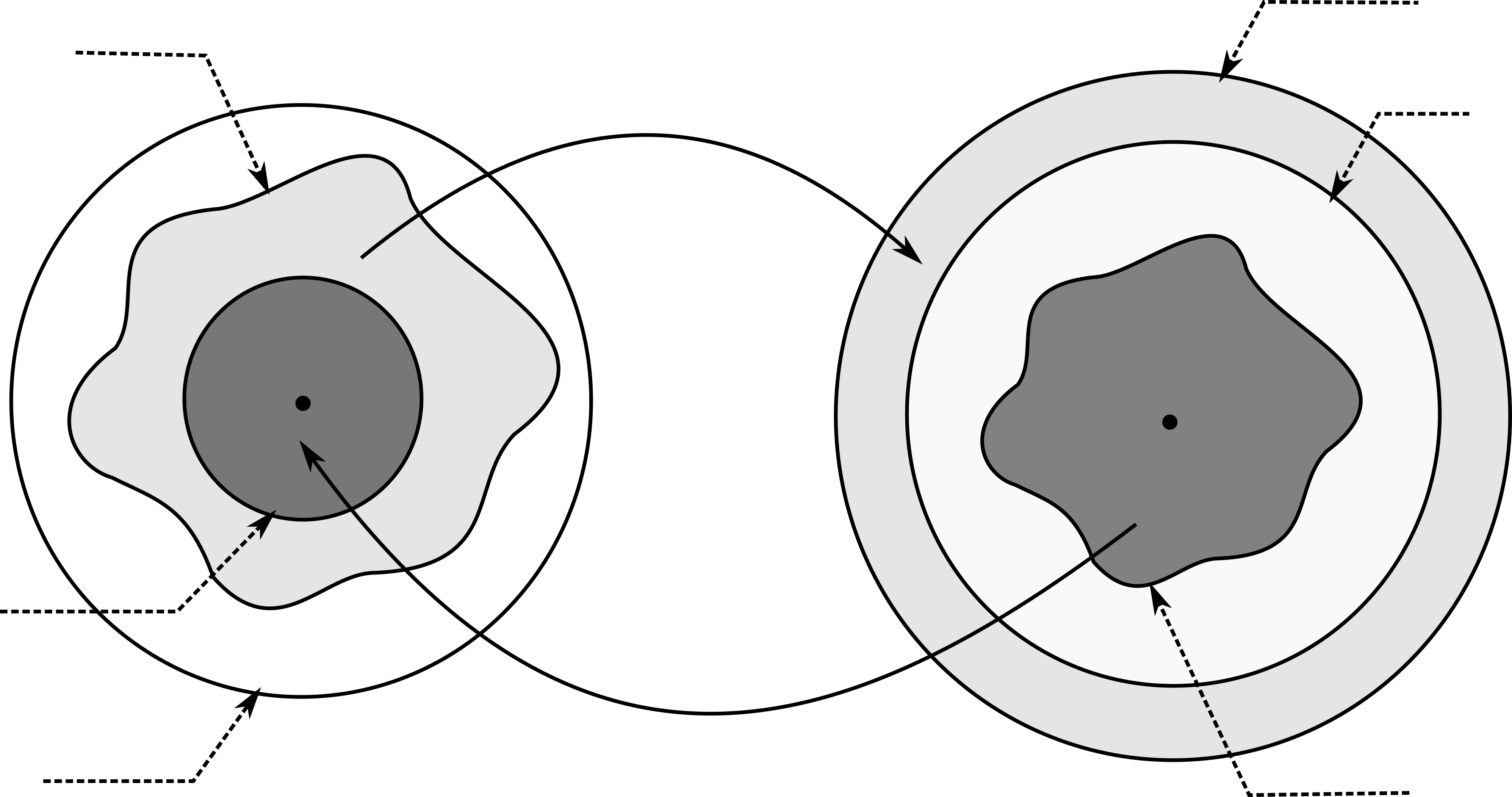
Refer to caption — Figure 1: Neighborhoods given in Corollary 3.5

Remark 3.6.

Here are some remarks on Theorem 3.3 and Corollary 3.5.

(3.6a)

Equation (3.1b) ensures uniqueness of $y_{x}$ . If one is only interested in showing the existence of $y_{x}$ , then one may relax (3.1) to just (3.1a).
(3.6b)

For finite-dimensional spaces, the bounds given by Corollary 3.5 are better than those given by Abraham et al. (Abraham et al. 2007, Proposition 2.5.6). : Proposition 2.5.6 from Abraham et al. 2007 provides the bounds for the estimates for the IFT. Bounds given by Corrolary 3.5 for the IFT are applicable on a larger domain than that of (Abraham et al. 2007, Proposition 2.5.6) and hence are superior.
(3.6c)

Since our objective is to come up with bounds that require minimal numerical computation, we relax several inequalities on the way and use conservative versions of them. For instance, we use Corollary 2.6 which is a coarser version of Theorem 2.5. Further, in several places, we utilize the submultiplicativity of norms to arrive at these results.
(3.6d)

The proof for Theorem 3.3 relies on constructing an approximation $\mathrm{Aff}(F)(\cdot;x)$ of the map $F(\cdot;x)$ and showing both of them are nonvanishingly homoptopic on $\bndry\mathsf{B}\left(y_{0},r_{y}\right)$ . One may improve the obtained estimates by approximating $F(\cdot;x)$ with a different function $\tilde{F}(\cdot~;x)$ and constructing homotopy $H^{\prime}$ such that $F$ and $\tilde{F}$ are nonvanishingly homotopic and then use analysis on $\tilde{F}$ to show the existence of solutions of $F(y;x)=0$ . We refer the reader to (Krasnoselʹskij and Zabrejko 1984, Chapter 1), in which Krasnosel’skij et al. have discussed several methods to come up with such homotopies.

In order to compute these estimates one needs to compute the second-order derivatives over a bounded region. In light of this, $f\in\mathcal{C}^{2}$ is a necessary requirement. However, for $\mathcal{C}^{1}$ maps, one can alternatively use the bounds on the first-order derivatives to come up with similar estimates. In Holtzman 1970, Holtzman provides explicit estimates for the Implicit function theorem (given by the following proposition). However, for finite-dimensional spaces, one can also obtain these estimates by degree theoretic ideas. We now present these estimates and a degree theoretic proof of the same.

Proposition 3.7.

(Holtzman 1970, Theorem) Let $\mathbb{R}^{n}\times\mathbb{R}^{m}\supset\Omega\ni(x,y)\longmapsto P(x,y)\in\mathbb{R}^{m}$ be a continuous map. Let $\Omega$ be open and $(x_{0},y_{0})\in\Omega$ . Assume:

(i)

$P(x_{0},y_{0})=0$ ;
(ii)

$\mathop{}\!\mathrm{D}_{y}P$ exists and is continuous in $\Omega$ ;
(iii)

$\mathop{}\!\mathrm{D}_{y}P(x_{0},y_{0})$ has bounded inverse $\Gamma=(\mathop{}\!\mathrm{D}_{y}P(x_{0},y_{0}))^{-1}$ and $\left\lVert\Gamma\right\rVert=k_{1}$ ;
(iv)

$S=\{(x,y)\in\mathsf{B}\left(x_{0},\delta\right)\times\cl\mathsf{B}\left(y_{0},\epsilon\right)\}\subset\Omega$ ;

(v)

there is a real-valued function $g_{1}(u,v)$ defined for $(u,v)\in[0,\delta]\times[0,\epsilon]$ and nondecreasing in each argument with the other fixed such that for all $(x,y)\in S$

\left\lVert\mathop{}\!\mathrm{D}_{y}P(x,y)-\mathop{}\!\mathrm{D}_{y}P(x_{0},y_{0})\right\rVert\leq g_{1}(\left\lVert x-x_{0}\right\rVert,\left\lVert y-y_{0}\right\rVert);

(vi)

there is a nondecreasing function $g_{2}$ defined on $[0,\delta]$ such that for all $(x,y)\in S$

$\left\lVert P(x,y_{0})\right\rVert\leq g_{2}(\left\lVert x-x_{0}\right\rVert);$
(vii)

$k_{1}g_{1}(\delta,\epsilon)\leq\alpha<1$ , and $k_{1}g_{2}(\delta)\leq\epsilon(1-\alpha)$ .

Then a unique map $F$ exists defined on $\mathsf{B}\left(x_{0},\delta\right)$ mapping into $\cl\mathsf{B}\left(y_{0},\epsilon\right)$ and possessing the following properties:

(a)

$P(x,F(x))=0$ for all $x\in\mathsf{B}\left(x_{0},\delta\right)$ .
(b)

$F(x_{0})=y_{0}$ .
(c)

$x\longmapsto F(x)$ is continuous.

Proof.

We first prove the strict version of (vii) and then using this we achieve the nonstrict version (vii). To this end, let $\epsilon>0$ and $\delta>0$ be such that $k_{1}g_{1}(\delta,\epsilon)<\alpha<1$ and $k_{1}g_{2}<\epsilon(1-\alpha)$ and $\mathsf{B}\left(x_{0},\delta\right)\times\cl\mathsf{B}\left(y_{0},\epsilon\right)\subset\Omega$ . Fix an $x\in\mathsf{B}\left(x_{0},\delta\right)$ and define $\cl\mathsf{B}\left(y_{0},\epsilon\right)\ni y\longmapsto P(y;x)\coloneqq P(x,y)-P(x_{0},y_{0})$ . Further, define an approximation of $P(\cdot;x)$ as

y\longmapsto\mathrm{Aff}(P)(y;x)\coloneqq P(x,y_{0})+\mathop{}\!\mathrm{D}_{y}P(x_{0},y_{0})\tilde{y}

(3.10)

where $\tilde{y}\coloneqq y-y_{0}$ and $\tilde{x}\coloneqq x-x_{0}$ . From definition of $P(\cdot;x)$ we have

\begin{split}P(y;x)-\mathrm{Aff}(P)(y;x)&=(P(x,y)-P(x,y_{0}))-\mathop{}\!\mathrm{D}_{y}P(x_{0},y_{0})\tilde{y}.\\ &=\int_{0}^{1}\Big(\mathop{}\!\mathrm{D}_{y}P(x,y_{0}+t\tilde{y})-\mathop{}\!\mathrm{D}_{y}P(x,y_{0})\Big)\tilde{y}\mathop{}\!\mathrm{d}t,\end{split}

and

\left\lVert P(y;x)-\mathrm{Aff}(P)(y;x)\right\rVert\leq\left(\int_{0}^{1}\left\lVert\mathop{}\!\mathrm{D}_{y}P(x,y_{0}+t\tilde{y})-\mathop{}\!\mathrm{D}_{y}P(x,y_{0})\right\rVert\mathop{}\!\mathrm{d}t\right)\left\lVert\tilde{y}\right\rVert.

Therefore, from (v), for all $y\in\bndry\mathsf{B}\left(y_{0},\epsilon\right)$

\left\lVert P(y;x)-\mathrm{Aff}(P)(y;x)\right\rVert\leq g_{1}(\delta,\epsilon)\epsilon\leq\frac{\alpha\epsilon}{k_{1}}.

(3.11)

Similarly, using (iii), (vi) and (3.10), for all $y\in\bndry\mathsf{B}\left(y_{0},\epsilon\right)$ we have

\left\lVert\mathrm{Aff}(P)(y;x)\right\rVert\geq\frac{\epsilon}{k_{1}}-g_{2}(\delta).

(3.12)

Since by assumption $k_{1}g_{2}(\delta)<\epsilon(1-\alpha)$ , from (3.11) and (3.12) we have

\left\lVert P(y;x)-\mathrm{Aff}(P)(y;x)\right\rVert<\left\lVert\mathrm{Aff}(P)(y;x)\right\rVert.

Thus using Corollary 2.6 we have

\mathrm{Deg}\left({P(\cdot;x)},{\mathsf{B}\left(y_{0},\epsilon\right)}\right)=\mathrm{Deg}\left({\mathrm{Aff}(P)(\cdot;x)},{\mathsf{B}\left(y_{0},\epsilon\right)}\right)\in\{-1,1\}.

Therefore, there exists a $y_{x}\in\mathsf{B}\left(y_{0},\epsilon\right)$ such that $P(x,y_{x})=0$ .

Following arguments similar to those of Theorem 3.3, for uniqueness, it suffices to show that $\mathop{}\!\mathrm{D}_{y}P(x,y)$ is nonsingular for all $(x,y)\in S$ . Rewriting $\mathop{}\!\mathrm{D}_{y}P(x,y)$ as

\mathop{}\!\mathrm{D}_{y}P(x,y)=\mathop{}\!\mathrm{D}_{y}P(x_{0},y_{0})\Big(\mathrm{I}_{n}-\Gamma(\mathop{}\!\mathrm{D}_{y}P(x_{0},y_{0})-\mathop{}\!\mathrm{D}_{y}P(x,y))\Big)

Using (vii), for all $(x,y)\in S$ ,

	$\displaystyle\left\lVert\Gamma\big(\mathop{}\!\mathrm{D}_{y}P(x_{0},y_{0})-\mathop{}\!\mathrm{D}_{y}P(x,y)\big)\right\rVert$	$\displaystyle\leq\left\lVert\Gamma\right\rVert\left\lVert\mathop{}\!\mathrm{D}_{y}P(x_{0},y_{0})-\mathop{}\!\mathrm{D}_{y}P(x,y)\right\rVert$
		$\displaystyle\leq k_{1}\alpha<1.$

Hence using Lemma 3.4, $\mathop{}\!\mathrm{D}_{y}P(x,y)$ is nonsingular for all $(x,y)\in S$ . Therefore for all $\epsilon>0$ , $\delta>0$ such that $k_{1}g_{1}(\delta,\epsilon)<\epsilon(1-\alpha)$ , for all $x\in\mathsf{B}\left(x_{0},\delta\right)$ there exists a unique $y_{x}\in\mathsf{B}\left(y_{0},\epsilon\right)$ such that $P(x,y_{x})=0$ .

For given $\delta>0$ , define

\epsilon^{*}\coloneqq\sup\left\{\epsilon\mid k_{1}g_{1}(\delta,\epsilon)\leq\alpha,~k_{1}g_{2}(\delta)\leq\epsilon(1-\alpha)\right\}>0.

Choose an $\alpha<\alpha^{\prime}<1$ , and extend $g_{1}$ , $g_{2}$ if necessary, then there exists an $\epsilon^{\prime}$ such that $k_{1}g_{1}(\delta,\epsilon^{\prime})<\alpha^{\prime}$ and $k_{1}g_{2}(\delta)<\epsilon^{\prime}(1-\alpha^{\prime})$ and $\mathsf{B}\left(x_{0},\delta\right)\times\mathsf{B}\left(y_{0},\epsilon^{\prime}\right)\in\Omega$ . One can see that $\epsilon^{\prime}>\epsilon^{*}$ . Set

\epsilon^{\prime\prime}(\alpha^{\prime})=\inf\left\{\epsilon^{\prime}\mid k_{1}g_{1}(\delta,\epsilon^{\prime})<\alpha^{\prime},~k_{1}g_{2}(\delta)<\epsilon^{\prime}(1-\alpha^{\prime})\right\}.

Then for each $x\in\mathsf{B}\left(x_{0},\delta\right)$ , there exist a unique $y_{x}\in\mathsf{B}\left(y_{0},\epsilon^{\prime\prime}(\alpha^{\prime})\right)$ such that $P(x,y_{x})=0$ . Let $\{\alpha_{n}\mid n\in\mathbb{N}\}$ be a monotone decreasing sequence with $\alpha_{n}\leq\alpha^{\prime}$ and $\alpha_{n}\longrightarrow\alpha$ . Suppose $g_{1}(\delta,\cdot)$ is continuous on $[\epsilon^{*},\epsilon^{\prime}]$ ²² 2 Such an extension of $g_{1}(\delta,\cdot)$ exists and one possible choice is $g_{1}(\delta,r)=\begin{cases}g_{1}(\delta,r)&~\quad r\leq\epsilon^{*},\\ g_{1}(\delta,\epsilon^{*})+\sup\left\{\left\lVert\mathop{}\!\mathrm{D}_{y}P(x,y)-\mathop{}\!\mathrm{D}_{y}P(x_{0},y_{0})\right\rVert\mid S_{r}\right\}&\\ -\sup\left\{\left\lVert\mathop{}\!\mathrm{D}_{y}P(x,y)-\mathop{}\!\mathrm{D}_{y}P(x_{0},y_{0})\right\rVert\mid S\right\}&~\quad r>\epsilon^{*},\end{cases}$ where $S_{r}=\mathsf{B}\left(x_{0},\delta\right)\times\mathsf{B}\left(y_{0},r\right)$ . then we have a sequence $\epsilon_{n}\coloneqq\epsilon^{\prime\prime}(\alpha_{n})$ , such that $\epsilon_{n}\longrightarrow\epsilon^{*}$ . Furthermore, for each $x\in\mathsf{B}\left(x_{0},\delta\right)$ , there exists a unique $y_{x}$ such that $P(x,y_{x})=0$ and for each $n$ , $y_{x}\in\mathsf{B}\left(y_{0},\epsilon_{n}\right)$ . Therefore

y_{x}\in\bigcap_{n\in\mathbb{N}}\mathsf{B}\left(y_{0},\epsilon_{n}\right)=\cl\mathsf{B}\left(y_{0},\epsilon^{*}\right).

Thus, for each $\delta,\epsilon$ satisfying (vii), for each $x\in\mathsf{B}\left(x_{0},\delta\right)$ there exists a unique $y_{x}\in\cl\mathsf{B}\left(y_{0},\epsilon\right)$ satisfying $P(x,y_{x})=0$ . Defining $x\longmapsto F(x)=y_{x}$ proves (a) and (b), while (c) is a consequence of Theorem 3.2 (ImFT). ∎

In Proposition 3.7, in addition to the above assumptions, if $\mathop{}\!\mathrm{D}_{x}P(x,y)$ exists and is continuous then one has the following corollary.

Corollary 3.8.

Let $U\subset\mathbb{R}^{n}$ and $V\subset\mathbb{R}^{m}$ be open sets and $U\times V\ni(x,y)\longmapsto f(x,y)\in\mathbb{R}^{n}$ be $\mathcal{C}^{1}$ . Suppose for some $(x_{0},y_{0})\in U\times V$ , $\mathop{}\!\mathrm{D}_{y}f(x_{0},y_{0})$ is an isomorphism. Define $M_{y}\coloneqq\left\lVert(\mathop{}\!\mathrm{D}_{y}f(x_{0},y_{0}))^{-1}\right\rVert$ and $L_{x}\coloneqq\left\lVert\mathop{}\!\mathrm{D}_{x}f(x_{0},y_{0})\right\rVert$ . For any given $r_{x}>0$ and $r_{y}>0$ define

	$\displaystyle\mathbf{L}_{x}(r_{x})$	$\displaystyle\coloneqq\sup\left\{\left\lVert\mathop{}\!\mathrm{D}_{x}f(x,y_{0})-\mathop{}\!\mathrm{D}_{x}f(x_{0},y_{0})\right\rVert\mid(x,y)\in\mathsf{B}\left(x_{0},r_{x}\right)\right\},\text{ and }$
	$\displaystyle\mathbf{L}_{y}(r_{x},r_{y})$	$\displaystyle\coloneqq\sup\left\{\left\lVert\mathop{}\!\mathrm{D}_{y}f(x,y)-\mathop{}\!\mathrm{D}_{y}f(x_{0},y_{0})\right\rVert\mid(x,y)\in\mathsf{B}\left(x_{0},r_{x}\right)\times\mathsf{B}\left(y_{0},r_{y}\right)\right\}.$

Then for all $r_{x}>0$ and $r_{y}>0$ satisfying


$\displaystyle\mathbf{L}_{x}(r_{x})r_{x}+\mathbf{L}_{y}(r_{x},r_{y})r_{y}$	$\displaystyle<\frac{r_{y}}{M_{y}}-L_{x}r_{x},\text{ and }$	(3.13a)
$\displaystyle M_{y}\mathbf{L}_{y}(r_{x},r_{y})\leq\alpha<1{,}$		(3.13b)

for each $x\in\mathsf{B}\left(x_{0},r_{x}\right)$ there exist a unique $y_{x}\in\mathsf{B}\left(y_{0},r_{y}\right)$ satisfying $f(x,y_{x})=w_{0}\eqqcolon f(x_{0},y_{0})$ . Furthermore, $\mathsf{B}\left(x_{0},r_{x}\right)\ni x\longmapsto g(x)\coloneqq y_{x}\in\mathsf{B}\left(y_{0},r_{y}\right)$ is continuously differentiable.

Proof.

Define $g_{1}(r_{x},r_{y})\coloneqq\mathbf{L}_{y}(r_{x}){r_{y}}$ and $g_{2}(r_{x})\coloneqq\mathbf{L}_{x}(r_{x})$ . Applying Proposition 3.7 with inequality (vii) replaced with its strict version and rearranging terms provide (3.13a) and (3.13b). The differentiability of $g$ is a consequence of Theorem 3.1 (ImFT). ∎

Corollary 3.9.

Let $U\subset\mathbb{R}^{n}$ be open and $U\ni x\longmapsto f(x)\in\mathbb{R}^{n}$ be a $\mathcal{C}^{1}$ map. Let $x_{0}\in U$ be such that $\mathop{}\!\mathrm{D}f(x_{0})$ is nonsingular. Define $L\coloneqq\left\lVert\mathop{}\!\mathrm{D}f(x_{0})\right\rVert$ and $M\coloneqq\left\lVert(\mathop{}\!\mathrm{D}f(x_{0}))^{-1}\right\rVert$ . For each $r>0$ , define

\mathbf{L}(r)\coloneqq\sup\left\{{\left\lVert\mathop{}\!\mathrm{D}f(x)-\mathop{}\!\mathrm{D}f(x_{0})\right\rVert}\mid x\in\mathsf{B}\left(x_{0},r\right)\right\}.

Then for all $r_{x}>0$ and $r_{y}>0$ satisfying

\mathbf{L}(r_{x}){<}\frac{1}{M}\quad\text{ and }\quad r_{y}=\frac{r_{x}(1-M\mathbf{L}(r_{x}))}{M},

there exist an open set $H_{r_{x}}\subset\mathsf{B}\left(x_{0},r_{x}\right)$ such that $f$ maps $H_{r_{x}}$ onto $\mathsf{B}\left(y_{0},r_{y}\right)$ $\mathcal{C}^{1}$ -diffeomorphically. Further, for each $0<r<r_{y}$ , define

\mathbf{M}(r)=\sup\left\{\left\lVert\mathop{}\!\mathrm{D}f^{-1}(y)-\mathop{}\!\mathrm{D}f^{-1}(y_{0})\right\rVert\mid y\in\mathsf{B}\left(y_{0},r\right)\right\}.

Then for each $r_{y}^{\prime}>0$ and $r_{x}^{\prime}>0$ satisfying

\mathbf{M}(r_{y}^{\prime}){<}\frac{1}{L}\quad\text{ and }\quad r_{x}^{\prime}=\frac{r_{y}{{}^{\prime}}(1-L\mathbf{M}(r_{y}^{\prime})}{L},

there exists an open set $H^{\prime}_{r_{y}^{\prime}}\subset\mathsf{B}\left(x_{0},r_{y}^{\prime}\right)$ such that $f^{-1}$ maps $H^{\prime}_{r_{y}^{\prime}}$ , $\mathcal{C}^{1}-$ diffeomorphically onto $\mathsf{B}\left(x_{0},r_{x}^{\prime}\right)\subset H_{r_{x}}$ .

Remark 3.10.

Estimating $\mathbf{M}$ requires explicit expression of $\mathop{}\!\mathrm{D}f^{-1}(y_{0})$ . This can be overcome by using the relation $\mathop{}\!\mathrm{D}f^{-1}(y)=(\mathop{}\!\mathrm{D}f(x))^{-1}$ , where $x=f^{-1}(y)$ . Let $r^{\prime}<r_{x}$ , be such that $r=r{{}^{\prime}}(1-M\mathbf{L}(r^{\prime}))/M$ , then we have

\mathbf{M}(r)\leq\sup\left\{\left\lVert(\mathop{}\!\mathrm{D}f(x))^{-1}-(\mathop{}\!\mathrm{D}f(x_{0}))^{-1}\right\rVert\mid x\in\mathsf{B}\left(x_{0},r^{\prime}\right)\right\}.

Corollary 3.5 and Corollary 3.9 considers an unconstrained variation around $y_{0}$ . However, often we are interested to know how the preimage of $y$ under $f$ varies when $y$ is varied along a particular direction. A slightly improved version of Corollary 3.5 is presented in the following proposition.

Proposition 3.11.

Let $U\subset\mathbb{R}^{n}$ be a nonempty open set and $f\colon U\longrightarrow\mathbb{R}^{n}$ satisfy the assumptions of Theorem 3.2 and $L$ , $M$ , $K$ , $P$ and $R$ be as defined in Corollary 3.5. Let $\mathsf{W}\subset\mathbb{R}^{n}$ be a subspace, define

\mathsf{B}_{\mathsf{W}}\left(y_{0},r_{\mathsf{W}}\right)\coloneqq\{y\subset\mathbb{R}^{n}\mid y-y_{0}\in\mathsf{W}~\text{and}~\left\lVert y-y_{0}\right\rVert<r_{\mathsf{W}}\}

and

M_{\mathsf{W}}\coloneqq\sup\left\{\left\lVert\mathop{}\!\mathrm{D}f^{-1}(y_{0}){\tilde{y}}\right\rVert\mid{\tilde{y}}\in\mathsf{B}_{\mathsf{W}}\left(0,1\right)\right\}.

Then for any

0{<}r_{x}<\min\left\{\frac{1}{MK},R\right\}\quad\text{ and }\quad r_{\mathsf{W}}=\frac{r_{x}(2-r_{x}MK)}{2M_{\mathsf{W}}},

for each $y\in\mathsf{B}_{\mathsf{W}}\left(y_{0},r_{\mathsf{W}}\right)$ , there exist a unique $x_{y}\in\mathsf{B}\left(x_{0},r_{x}\right)\subset\mathbb{R}^{n}$ such that $f(x_{y})=y$ .

Proof.

First fix a $y\in\mathsf{B}_{\mathsf{W}}\left(y_{0},r_{\mathsf{W}}\right)$ and define $F(x;y)=(\mathop{}\!\mathrm{D}f{x_{0}})^{-1}(f(x)-y)$ . We have $F(x;y)=0\iff f(x)=y$ . Define an approximation of $F(\cdot;y)$ as

\mathrm{Aff}(F)(x;y)=(x-x_{0})-\mathop{}\!\mathrm{D}f(x_{0})^{-1}(y-y_{0}).

Setting $\tilde{x}\coloneqq x-x_{0}$ and $\tilde{y}\coloneqq y-y_{0}$ we have

	$\displaystyle F(x;y)-\mathrm{Aff}(F)(x;y)$	$\displaystyle=\mathop{}\!\mathrm{D}f(x_{0})^{-1}(f(x-y))-(\tilde{x}-\mathop{}\!\mathrm{D}f(x_{0})^{-1}\tilde{y})$
		$\displaystyle=\mathop{}\!\mathrm{D}f(x_{0})^{-1}\Big(f(x)-\big(f(x_{0})+\mathop{}\!\mathrm{D}f(x_{0})\tilde{x}\big)\Big).$

Therefore,

\left\lVert F(x;y)-\mathrm{Aff}(F)(x;y)\right\rVert<\frac{1}{2}MKr_{x}^{2}~\text{ for all }~x\in\mathsf{B}\left(x_{0},r_{x}\right).

Similarly,

	$\displaystyle\left\lVert\mathrm{Aff}(F)(x;y)\right\rVert$	$\displaystyle=\left\lVert\tilde{x}-\mathop{}\!\mathrm{D}f(x_{0})^{-1}\tilde{y}\right\rVert$
		$\displaystyle\geq\left\lvert\left\lVert\tilde{x}\right\rVert-\left\lVert\mathop{}\!\mathrm{D}f(x_{0})^{-1}\tilde{y}\right\rVert\right\lvert$
		$\displaystyle>r_{x}-M_{\mathsf{W}}r_{\mathsf{W}}~\text{ for all }~x\in\bndry\mathsf{B}\left(r_{x},.\right)$

Then for all $r_{x}$ and $r_{\mathsf{W}}$ satisfying

\frac{1}{2}MKr_{x}^{2}\leq r_{x}-M_{\mathsf{W}}r_{\mathsf{W}}

(3.14)

we have (for all $y\in\mathsf{B}_{\mathsf{W}}\left(y_{0},r_{\mathsf{W}}\right)$ ) $\left\lVert F(x;y)-\mathrm{Aff}(F)(x;y)\right\rVert<\left\lVert\mathrm{Aff}(F)(x;y)\right\rVert$ for all $x\in\bndry\mathsf{B}\left(x_{0},r_{x}\right)$ and therefore are nonvanishingly homotopic. Therefore,

\mathrm{Deg}\left({F(\cdot;y)},{\mathsf{B}\left(x_{0},r_{x}\right)}\right)=\mathrm{Deg}\left({\mathrm{Aff}(F)(\cdot;y)},{\mathsf{B}\left(x_{0},r_{x}\right)}\right)\in\{-1,1\},

and thus there exists $x_{y}\in\mathsf{B}\left(x_{0},r_{x}\right)$ such that $F(x_{y};y)=0\iff f(x_{y})=y$ . This proves existence of such an $x_{y}\in\mathsf{B}\left(x_{0},r_{x}\right)$ for each $y\in\mathsf{B}_{\mathsf{W}}\left(y_{0},\mathsf{r_{\mathsf{W}}}\right)$ . Since for all $r_{x}<\min\{\frac{1}{MK},R\}$ , $\mathop{}\!\mathrm{D}F(x;y)=\mathop{}\!\mathrm{D}f(x_{0})^{-1}\mathop{}\!\mathrm{D}f(x)$ is invertible for all $x\in\mathsf{B}\left(x_{0},r_{x}\right)$ , the uniqueness of $x_{y}$ is asserted following arguments similar to Proposition 3.5. For a given $r_{x}$ , maximizing $r_{\mathsf{W}}$ while satisfying (3.14) results in the equality

r_{\mathsf{W}}=\frac{r_{x}(2-r_{x}MK)}{2M_{\mathsf{W}}},

(3.15)

and thereby completing the proof. ∎

4 Applications

ImFT and IFT find their applications in proving several results in nonlinear analysis and form the basis of several results in system theory and control, such as the robustness of solutions, and the existence, and uniqueness of solutions of ordinary differential equations. Several existential results on robustness are a consequence of the ImFT. One can apply the bounds derived in this article on the ImFT and IFT to obtain quantitative variants of the aforementioned methods. In this section, we include two such applications. First, we look into the robustness of the solutions of the nonlinear equations with respect to parametric variations and particularly the Quadrartically constrained Quadratic Programs (QCQP). A second application of these bounds is in geometric control methods, where we utilize these bounds to give explicit estimates on the domain of the feedback linearization of discrete-time dynamical systems.

4.1 Robustness of Nonlinear Equations

Solving nonlinear equations is challenging, and one often needs to employ numerical methods to compute a solution for a system of nonlinear equations. Estimates of the bounds in the ImFT and IFT help in proving the existence of solutions for a system of nonlinear equations on a given set, as we now demonstrate.

Let $f\colon\mathbb{R}^{n}\times\mathbb{R}^{m}\longrightarrow\mathbb{R}^{n}$ be a $\mathcal{C}^{2}$ map. Let $X\subset\mathbb{R}^{n}$ , $U\subset\mathbb{R}^{m}$ be nonempty open sets. A system of nonlinear equations in $(x,u)$ on $X\times U$ is given by

f(x,u)=0

(4.1)

is solvable if there exists an $(x_{0},u_{0})\in X\times U$ such that $f(x_{0},u_{0})=0$ .

Definition 4.1.

Let $\Omega\subset X$ have a nonempty interior. (4.1) is said to be robustly solvable on $\Omega$ , if there exists an $r_{u}>0$ , such that for all $u\in\mathsf{B}\left(u_{0},r_{u}\right)\subset U$ , there exists a (unique) $x_{u}\in\Omega$ satisfying $f(x_{u},u)=0$ . Moreover, for a given $r_{x}$ , the supremum over all such $r_{u}$ s is called the robustness margin for (4.1) over $\Omega$ .

Remark 4.2.

Definition 4.1 is similar to (Dvijotham et al. 2019, Definition 2.1). However, unlike (Dvijotham et al. 2019, Definition 2.1), $\Omega$ can be arbitrarily chosen and need not arise from linear constraints given by equation (2) in Dvijotham et al. 2017.

Theorem 4.3.

Let $X\subset\mathbb{R}^{n},~U\subset\mathbb{R}^{m}$ be nonempty set and $f:X\times U\longrightarrow\mathbb{R}^{n}$ be a $\mathcal{C}^{2}$ map. Let $(x_{0},u_{0})\in X\times U$ be such that $f(x_{0},u_{0})=0$ and $\mathop{}\!\mathrm{D}_{x}f(x_{0},u_{0})$ is nonsingular. Define

L_{u}\coloneqq\left\lVert\mathop{}\!\mathrm{D}_{u}f(x_{0},u_{0})\right\rVert\quad\text{ and }\quad M_{x}\coloneqq\left\lVert\left(\mathop{}\!\mathrm{D}_{x}f(x_{0},u_{0})^{-1}\right)\right\rVert

and for a given $R_{x}>0,R_{u}>0$ such that $\mathsf{B}\left(x_{0},R_{x}\right)\subset X$ and $\mathsf{B}\left(u_{0},R_{u}\right)\subset U$ set

	$\displaystyle K_{xx}$	$\displaystyle\coloneqq\sup\left\{\left\lVert\mathop{}\!\mathrm{D}^{2}_{x}f(x,u)\right\rVert\mid(x,u)\in\mathsf{B}\left(x_{0},R_{x}\right)\times\mathsf{B}\left(u_{0},R_{u}\right)\right\},$
	$\displaystyle K_{uu}$	$\displaystyle\coloneqq\sup\left\{\left\lVert\mathop{}\!\mathrm{D}^{2}_{x}f(x,u)\right\rVert\mid(x,u)\in\mathsf{B}\left(x_{0},R_{x}\right)\times\mathsf{B}\left(u_{0},R_{u}\right)\right\},\text{ and }$
	$\displaystyle K_{xu}$	$\displaystyle\coloneqq\sup\left\{\left\lVert\mathop{}\!\mathrm{D}_{x}\mathop{}\!\mathrm{D}_{u}f(x,u)\right\rVert\mid(x,u)\in\mathsf{B}\left(x_{0},R_{x}\right)\times\mathsf{B}\left(u_{0},R_{u}\right)\right\}.$

Then for all $r_{x}$ and $r_{u}$ satisfying


$\displaystyle\frac{1}{2}K_{xx}r_{x}^{2}+K_{xu}r_{x}r_{u}+\frac{1}{2}K_{uu}r_{u}^{2}$	$\displaystyle<\frac{r_{x}}{M_{x}}-L_{u}r_{u},$	(4.2a)
$\displaystyle K_{xu}r_{u}+K_{xx}r_{x}$	$\displaystyle<\frac{1}{M_{x}},$	(4.2b)
$\displaystyle 0<r_{u}$	$\displaystyle\leq R_{x},\text{ and }$	(4.2c)
$\displaystyle 0<r_{x}$	$\displaystyle\leq R_{y},$	(4.2d)

(4.1) is robustly solvable on $\mathsf{B}\left(x_{0},r_{x}\right)$ and robustness margin is bounded below by $r_{u}$ .

Remark 4.4.

Similar to Theorem 3.3, (4.2b) is necessary for the uniqueness of the solution. If the uniqueness is not required then one can relax (4.2) to (4.2a), (4.2c) and (4.2d).

The proof follows directly from applying Theorem 3.3 on $f$ , and is therefore omitted. With the general nonlinear case described, we now consider the QCQPs.

4.1.1 Robustness of Solutions of QCQPs

Let $u\in\mathbb{R}^{n}$ and define

\mathbb{R}^{n}\ni x\longmapsto F(x)\coloneqq Q(x)+Lx\in\mathbb{R}^{n},

where $L\in\mathbb{R}^{n\times n}$ and $Q(x)$ is a quadratic function with its $i^{\text{th}}$ component defined as

[Q(x)]_{i}\coloneqq x^{\top}Q_{i}x~\text{for all}~i\in[n].

(4.3)

where for all $i\in[n]$ , $Q_{i}\in\mathbb{R}^{n\times n}$ is a symmetric matrix. For a given matrix $A$ and a vector $b$ , a QCQP is defined by a system of quadratic equations

F(x)=Q(x)+Lx=u,

(4.4)

subjected to $m$ constraints

x\in{\Omega}\coloneqq\{x\in\mathbb{R}^{n}~\mid~[Ax]_{i}\leq b_{i}~i\in[m]\},

(4.5)

where $[Ax]_{i}$ and $b_{i}$ denotes the $i^{\text{th}}$ components of the vectors $Ax$ and $b$ . The constraint set ${\Omega}$ defines a polyhedron as shown in Figure 2. The dashed lines represent the equalities $[Ax]_{i}=b_{i}$ and the shaded interior along with the boundary defines the constraint set.

It is assumed that the constraints are not redundant, and $x$ and $u$ have the same dimension. We are interested in the following problem.

Problem 4.5.

For a given $u_{0}$ , let there be an $x_{0}\in{\Omega}$ such that $(x_{0},u_{0})$ solves (4.4). Find the robustness margin, i.e., the largest $r_{u}{>}0$ such that for all $u$ satisfying $\Big\lvert[u_{0}]_{i}-[u]_{i}\Big\rvert{<}r_{u}$ for all $i\in[n]$ , there exists an $x\in{\Omega}$ (not necessarily unique) such that $(x,u)$ solves (4.4).

First we utilize the ImFT to show that a nonzero robustness margin exists and then use the bounds derived for ImFT to come up with a lower bound on $r_{u}$ . Casting (4.4) as (4.1), define

\mathbb{R}^{n}\times\mathbb{R}^{n}\ni(x,u)\longmapsto f(x,u)\coloneqq Q(x)+Lx-u\in\mathbb{R}^{n}.

(4.6)

The Jacobian for $f$ at $(x_{0},u_{0})$ is given by

\mathop{}\!\mathrm{D}f(x_{0},u_{0})=\begin{pmatrix}\mathop{}\!\mathrm{D}_{x}f(x_{0},u_{0}),&\mathop{}\!\mathrm{D}_{u}f(x_{0},u_{0})\end{pmatrix}=\begin{pmatrix}2Q^{\prime}(x_{0})+L,&\mathrm{I}_{n}\end{pmatrix}

(4.7)

where $Q^{\prime}(x_{0})$ denotes an ${n\times n}$ matrix with its $i^{\text{th}}$ row as $x_{0}^{\top}Q_{i}$ and $\mathrm{I}_{n}$ denotes an identity matrix of order $n$ . Since the inequalities are placed component-wise, i.e., we are looking for an $n$ -cube around $u_{0}$ , and ${\Omega}$ is defined by (4.5). We shall choose the infinity norm to work with, for a vector $v\in\mathbb{R}^{n}$ the infinity norm is defined as

\left\lVert v\right\rVert_{\infty}\coloneqq\max\left\{\lvert v_{i}\rvert\mid i\in[n]\right\}.

The corresponding induced norm is defined as follows: let $A\colon\mathbb{R}^{n}\times\mathbb{R}^{m}$ be a linear operator, then $\left\lVert A\right\rVert_{\infty}$ is defined as

\left\lVert A\right\rVert_{\infty}\coloneqq\max\left\{\left\lVert Ax\right\rVert_{\infty}\mid\left\lVert x\right\rVert_{\infty}\leq 1\right\}.

Let $\mathbb{R}^{n}\times\mathbb{R}^{n}\ni(u,v)\longmapsto B(u,v)\in\mathbb{R}^{m}$ be a bilinear map. The induced norm on $B$ is defined as

\left\lVert B\right\rVert_{\infty}\coloneqq\max\left\{\left\lVert B(u,v)\right\rVert_{\infty}\mid\left\lVert u\right\rVert_{\infty}\leq 1,~\left\lVert v\right\rVert_{\infty}\leq 1\right\}.

With this premise set, we have the following result.

Theorem 4.6.

Suppose $Q\in\mathbb{R}^{n\times n}\text{ and }L\in\mathbb{R}^{n\times n}$ is such that $2Q^{\prime}(x_{0})+L$ is non-singular, and ${\Omega}$ is nondegenerate, i.e., has a nonempty interior. Then (4.4) is robustly solvable on ${\Omega}$ . Moreover, define $M_{x}\coloneqq\left\lVert(2Q^{\prime}(x_{0})+L)^{-1}\right\rVert_{\infty}$ and $K_{xx}\coloneqq\max\left\{{\lvert x^{\top}Q_{i}x\rvert}\mid\left\lVert x\right\rVert_{\infty}=1,i\in[n]\right\}$ . Then for a given $0<r_{x}<\frac{1}{M_{x}K_{xx}}$ such that $\mathsf{B}\left(x_{0},r_{x}\right)\subset{\Omega}$ , the robustness margin $r_{u}$ is lower bounded by $\frac{r_{x}(2-M_{x}K_{xx}r_{x})}{2M_{x}}$ .

The proof is a straight forward application of Theorem 3.3 on $f$ as defined in (4.6) and hence omitted.

Remark 4.7.

The condition $0<r_{x}<1/M_{x}K_{xx}$ ensures uniqueness of $x\in\mathsf{B}\left(x_{0},1/M_{x}K_{xx}\right)$ . However, one can not assert the uniqueness of $x$ on $\Omega$ , using Theorem 4.6.

Example 4.8.

In order to illustrate the above calculated bounds we present a simple example. The example is taken from Dvijotham et al. 2019 so as to establish comparisons. The data is as follows:

A=\begin{bmatrix}-1&0\\ {1}&0\\ 0&{-1}\\ 0&1\end{bmatrix},~B=\begin{bmatrix}-0.5\\ 3\\ -0.5\\ 3\end{bmatrix},~Q_{1}=\begin{bmatrix}1&0\\ 0&0\end{bmatrix}~,Q_{2}=\begin{bmatrix}0&0\\ 0&1\end{bmatrix},~L=\begin{bmatrix}1&-3\\ 2&-1\end{bmatrix},\text{ and}~u_{0}=\begin{bmatrix}-2\\ 4\end{bmatrix}.

The underlying expression is then given by

F(x)=\begin{bmatrix}x_{1}^{2}+x_{1}-3x_{2}\\ x_{2}^{2}+2x_{1}-x_{2}\end{bmatrix}=\begin{bmatrix}-2\\ 4\end{bmatrix}\quad\text{with}\quad{\Omega}=\left\{x\colon\begin{bmatrix}0.5\\ 0.5\end{bmatrix}\leq\begin{bmatrix}x_{1}\\ x_{2}\end{bmatrix}\leq\begin{bmatrix}3\\ 3\end{bmatrix}\right\}.

(4.8)

The unique solution is given by $x_{0}\approxeq\begin{bmatrix}1.36&1.74\end{bmatrix}^{\top}$ . One can check that $\mathop{}\!\mathrm{D}F(x_{0})$ is nonsingular. The corresponding quantities are $L_{x}=6.7204$ , $M_{x}=0.3763$ , $L_{u}=1$ , and $K_{xx}=2$ . For ${r_{x}}=0.86$ , $\mathsf{B}\left(x_{0},0.86\right)\subset{\Omega}$ . The robustness margin for (4.8) comes out to be, $r_{u}\geq 1.546$ . This is greater than the estimates given by LP-feasibility routine ( $r_{u}\geq 1.2054$ ) by Dvijotham et al. in Dvijotham et al. 2019. The bounds can be further improved by changing the map $(x,u)\longmapsto(F(x)-u)$ to $\bar{F}(x,u)\coloneqq(\mathop{}\!\mathrm{D}F(x_{0})^{-1})\cdot(F(x)-u)$ . This gives us an updated bound of $r_{u}\geq 1.5781$ , however, this is smaller than the estimate given by the bound tightening procedure ( $r_{u}\geq 1.7069$ ) in Dvijotham et al. 2019. Figure 3 shows simulation results for the improved bounds. The blue scatter plot shows $F(\Omega)$ . The yellow rectangle shows the $\bndry\mathsf{B}\left(u_{0},r_{u}\right)$ . One can see that $\mathsf{B}\left(u_{0},r_{u}\right)$ is contained in $F(\Omega)$ and thus for each $u\in\mathsf{B}\left(u_{0},r_{u}\right)$ there will be an $x\in\omega$ such that $F(x)-u=0$ . The bounds can be improved if one restricts the variation along a particular subspace. This is shown by the purple-colored parallelogram. The $u$ was successively allowed to vary along an arbitrary unit vector $(w_{1},w_{2})$ , and the maximum perturbation was computed. This is denoted by $\bndry(B_{W})$ in the figure.

4.1.2 Application to Power Systems

Power Flow studies and Optimal Power Flow studies require us to calculate operating voltages and currents by balancing the load demand and the power generated. Integration of renewable sources like solar and wind energy in the power system network leads to uncertainty in the generated supply. Due to this uncertain supply of renewable sources, it is difficult to ensure that there will be sufficient power generation to meet the power demand while adhering to the stable operation limits of the power system network. The Power Flow equations involve balancing the generated power supply and the required demand. As described by Dvijotham et al. Dvijotham et al. 2017, the AC Power Flow equations are written as follows

\begin{split}\real\left(V_{i}\overline{Y_{i0}V_{0}}+\sum_{k=1}^{n}V_{i}\overline{Y_{ik}V_{k}}\right)&=p_{i}\quad\text{ for all }i\in\mathrm{PQ},\\ \imaginary\left(V_{i}\overline{Y_{i0}V_{0}}+\sum_{k=1}^{n}V_{i}\overline{Y_{ik}V_{k}}\right)&={q_{i}},\quad\text{ for all }i\in\mathrm{PQ},\\ \real\left(V_{i}\overline{Y_{i0}V_{0}}+\sum_{k=1}^{n}V_{i}\overline{Y_{ik}V_{k}}\right)&=p_{i}\quad\text{ for all }i\in\mathrm{PV},\\ \lvert V_{i}\lvert^{2}&=v_{i}^{2}\quad\text{ for all }i\in\mathrm{PV},\end{split}

(4.9)

where $V_{i}$ denotes the complex voltage phasor, $p_{i},~q_{i}$ denotes the active and reactive power injection at the node $i$ , and $Y$ denotes the admittance matrix. $\mathrm{PV}$ denotes the set of generator buses, and $\mathrm{PQ}$ denotes the load bus. $v_{i}$ denotes the root mean square (rms) voltage at the $i^{\text{th}}$ bus. $V_{0}$ denotes the reference slack bus and is kept fixed at $1+j0$ per unit magnitude, where $j=\sqrt{-1}$ . Power Flow as given by 4.9 is quadratic. Further, for stable operation of the power system network, one needs to maintain the bus voltage magnitude within prescribed limits. This imposes a quadratic constraint on (4.9). Setting

	$\displaystyle x$	$\displaystyle=\begin{bmatrix}\real(V_{1})&\ldots&\real(V_{n})&\imaginary(V_{1})&\ldots&\imaginary(V_{n})\end{bmatrix}\text{ and}$
	$\displaystyle u$	$\displaystyle=\begin{bmatrix}p_{1}&\ldots&p_{n}&q_{1}&\ldots&q_{n}&v_{1}^{2}&\ldots&v_{n}^{2}\end{bmatrix}$

the powerflow equations given by (4.9) can be written as QCQP of type (4.5) with $\mathbb{R}^{2n}\ni x\longmapsto F(x)\in\mathbb{R}^{2n}$ with its $i^{\text{th}}$ component given by

\begin{split}[F(x)]_{i}&\coloneqq\real\left(\sum_{k=1}^{n}V_{i}\overline{Y_{i0}V_{0}}+\overline{V_{i}Y_{ik}V_{k}}\right)\quad\text{ for all }i\in[n],\\ [F(x)]_{n+i}&\coloneqq\imaginary\left(V_{i}\overline{Y_{i0}V_{0}}+\sum_{k=1}^{n}V_{i}\overline{Y_{ik}V_{k}}\right)\quad\text{ for all }i\in\mathrm{PQ},\\ [F(x)]_{n+i}&\coloneqq{\real(V_{i})}^{2}+{\imaginary(V_{i})}^{2}\quad\text{ for all }i\in\mathrm{PV}.\end{split}

(4.10)

For stable operation, the voltage magnitudes are to be kept within tolerance limits. For a fixed $r_{x}\in]0,1[$ , the constraint set is

{\Omega}=\{x\in\mathbb{R}^{2n}\mid 1-r_{x}\leq v_{i}^{2}\leq 1+r_{x}~\text{for all}~i\in[n]\}.

The constraint set ${\Omega}$ can be relaxed to the following

{\Omega}^{\prime}=\{x\in\mathbb{R}^{2n}\mid-r_{x}\leq\left\lVert x-x^{*}\right\rVert_{\infty}\leq r_{x}~\text{for all}~i\in[n]\}

where $x^{*}\in\mathbb{R}^{2n}$ be the nominal operating point satisfying $(\real{V_{i}^{*}})^{2}+\imaginary({V_{i}^{*}})^{2}=1$ for all $i\in[n]$ .

The test cases are obtained from the dataset given in the MatPower package found in MATLAB software Zimmerman et al. 2010. The package contains well-defined libraries and a set of routines for solving problems like Power Flow analysis, Optimal Load Flow, and DC Power Flow analysis. The package is open source and is available online. The problem is simulated for several test cases from MatPower. The maximum allowable $r_{x}$ and $r_{u}$ are recorded in P.U. magnitude. In order to simulate real-life scenarios, we only consider the variation in the first five dimensions of $u$ . The results are tabulated in Table 1, where $M_{f}\coloneqq\left\lVert\mathop{}\!\mathrm{D}F^{-1}(u_{0})\right\rVert$ , $M_{F}^{\prime}\coloneqq\sup\left\{\mathop{}\!\mathrm{D}F^{-1}(u_{0})\cdot\tilde{u}\mid u\in\mathbb{R}^{2n},~\tilde{u}_{i}=0~\text{for all}~i>5\right\}$ , and $K_{\bar{F}}=\sup\left\{\left\lVert\mathop{}\!\mathrm{D}^{2}\bar{F}(x)\right\rVert\mid x\in\mathbb{R}^{2n}\right\}$ where $\bar{F}=(\mathop{}\!\mathrm{D}F(x_{0}))^{-1}\cdot F$ . For Case 5, 9, 14, and 30, we also plot $r_{x}$ with respect to $r_{u}$ and compare it with the bounds given by the bound tightening method given by Dvijotham et al. Dvijotham et al. 2019. These are shown in Figure. 4

Case	$M_{F}$	$M_{F}^{\prime}$	$K_{\bar{F}}$	Max $r_{x}$	Max $r_{u}$
5	0.5154	0.0512	12.971	0.0771	0.7529
9	1.3802	0.7968	39.065	0.0256	0.0161
14	2.4795	0.5291	91.066	0.0110	0.0104
30	6.2576	0.3225	0.330 $\times 10^{3}$	3.303 $\times 10^{-3}$	5.120 $\times 10^{-3}$
57	12.153	0.2657	1.032 $\times 10^{3}$	0.969 $\times 10^{-3}$	1.823 $\times 10^{-3}$
85	5.1119	0.0140	13.48 $\times 10^{3}$	0.074 $\times 10^{-3}$	2.643 $\times 10^{-3}$
141	22.049	0.2371	1.958 $\times 10^{3}$	0.512 $\times 10^{-3}$	1.078 $\times 10^{-3}$

Table 1: Lower bounds on the robustness margin

r_{u}

for various cases from MatPower

Remark 4.9.

From Table 1 and Figure 4, one can see, for lower values of $r_{x}$ , our bounds are comparable to those of Dvijotham et al. 2019. However, with an increase in the dimension, our estimates start to perform poorly as compared to those given in Dvijotham et al. 2019. The one key reason for this is the way we bound $K_{xx}$ . In order to keep computation minimum we bound $\max\left\{\lvert x^{\top}Qx\rvert\mid\left\lVert x\right\rVert_{\infty}\leq 1\right\}$ by $\sum_{i,n\in[n]}\lvert Q_{ij}\rvert$ . For a general matrix $Q$ this grows quadratically with respect to $n$ . However, if $Q$ is a sparse matrix, then one can obtain tighter estimates. One can alternatively utilize the inequlaity

\max\left\{\lvert x^{\top}Qx\rvert\mid\left\lVert x\right\rVert_{\infty}\leq 1\right\}\leq j\left\lVert Q\right\rVert_{2},

to estimate which grows linearly with $n$ .

Further, with an increase in $n$ , the problem dimension increases and norm-based inequalities such as triangular inequality and sub-multiplicative inequality become more conservative. Our estimates are conservative when compared to those provided in Dvijotham et al. 2019. However, the numerical computation required to compute these bounds is much lower than that required by Dvijotham et al. 2019. In particular, no optimization routine is required to compute these bounds. The bounds given by Dvijotham et.al. in Dvijotham et al. 2019 require us to perform nontrivial optimizations on matrices and solve LP feasibility programs. In comparison to that, we only require to compute for the inverse of an $n\times n$ matrix i.e., $\mathop{}\!\mathrm{D}F(x_{0})$ , for which there exist efficient algorithms and packages in literature. Since our objective is not to tackle matrix inversion methods, we do not investigate methods for computing matrix inversion. Some literature on matrix inversion can be found in Chern and Murata 1983; Martinsson et al. 2005; Li 2009; Liu et al. 2016. One key limitation of this method is that it can only provide us with a lower bound on the robustness margin.

4.1.3 Robustness of the Algebraic Riccati Equation

Consider a linear time invariant control system

\frac{\mathrm{d}x}{\mathrm{d}t}=Ax(t)+Bu(t)

(4.11)

with $x(t)\in\mathbb{R}^{n}$ , $u(t)\in\mathbb{R}^{m}$ for all $t>0$ . For any given $n\in\mathbb{N}$ , $\mathsf{Sym}(n)$ , $\mathsf{PD}(n)$ , and $\mathsf{PSD}(n)$ denotes the set of symmetric matrices, positive definite matrices, and positive semidefinite matrices of order $n\times n$ respectively. Let

\mathcal{U}=\bigg\{[0,\infty[\ni t\longmapsto u(t)\in\mathbb{R}^{m}\mid\int_{0}^{\infty}\left\lVert u(t)\right\rVert^{2}\mathop{}\!\mathrm{d}t<\infty\bigg\}~,

be the set of square integrable controls over infinite horizon. Define the infinite horizon Linear Quadratic Regulator (LQR) as the following optimal control problem.

Problem 4.10.

For given $Q\in\mathsf{PSD}(n),{\text{ and }}R\in\mathsf{PD}(m)$ compute a $u^{*}$ , if it exists, such that it solves

\begin{cases}\underset{u\in\mathcal{U}}{\minimize}\quad&J(u)=\frac{1}{2}\int_{0}^{\infty}x(t)^{\top}Qx(t)+u(t)^{\top}Ru(t),\\ \\ \text{subject to}\quad&x(0)=x_{0},\text{ and }\eqref{lin_are}\text{ for almost all }t\in[0,\infty[~.\end{cases}

From results on LQR (D.Liberzon 2011, Chapter 6), the optimal control is of the type

u^{*}(t)=-R^{-1}B^{\top}Px^{*}(t)~\quad\text{ for almost all }t\in[0,\infty[{,}

where $P\in\mathsf{PD}(n)$ solves the Algebraic Riccati Equation (ARE)

A^{\top}P+PA+Q-PBR^{-1}B^{\top}P=0{.}

(ARE)

For given $A_{0}\in\mathbb{R}^{n\times n}$ , and $B_{0}\in\mathbb{R}^{n\times m}$ such that $(A_{0},B_{0})$ forms a stabilizable pair, consider a linear control system given by

\frac{\mathrm{d}x}{\mathrm{d}t}=(A_{0}+\Lambda)x+B_{0}u

(4.12)

where parameter $\Lambda\in\mathbb{R}^{n\times n}$ denotes the unmodelled part of system dynamics.

Problem 4.11.

Find a bound on $\left\lVert\Lambda\right\rVert$ such that (4.12) is stabilizable, i.e., find an $r_{\Lambda}$ such that $(A_{0}+\Lambda,B_{0})$ is stabilizable for all $\Lambda\in\mathsf{B}\left(0,r_{\Lambda}\right)$ .

Remark 4.12.

Note that we may have very well considered variations in $B_{0}$ as well, however for illustration purposes, we restrict to variations in $A_{0}$ .

Lemma 4.13.

(D.Liberzon 2011, Chapter 6) For each $Q\in\mathsf{PD}(n)$ and $R\in\mathsf{PD}(m),$ a unique positive definite solution for (ARE) exists if and only if $(A,B)$ forms a stabilizable pair³³ 3 Two given matrices $A\in\mathbb{R}^{n\times n}$ and $B\in\mathbb{R}^{m\times n}$ are said to form a stabilizable pair if there exists a $K\in\mathbb{R}^{n\times m}$ such that $A+BK$ is Hurwitz i.e., have eigenvalues with strictly negative real parts..

Using the above lemma, for any given $\Lambda$ , $(A_{0}+\Lambda,B_{0})$ being stabilizable is equivalent to showing that (ARE) has a positive definite solution with $A=A_{0}+\Lambda$ . Further, since $\mathsf{PD}(n)$ is open in $\mathsf{Sym}(n)$ , there exists an $r_{P}$ such that for all $P\in\mathsf{B}\left(P_{0},r_{P}\right)\subset\mathsf{Sym}(n)$ , $P$ is positive definite. Problem 4.11 can now be formulated as the following robustness problem.

Problem 4.14.

For given $A_{0},B_{0},Q,R$ , let there be a $P_{0}\in\mathsf{PD}(n)$ such that it solves (ARE). For a given $r_{P}>0$ such that $\mathsf{B}\left(P_{0},r_{P}\right)\subset\mathsf{PD}(n)$ , find an $r_{\Lambda}>0$ such that for each $A\in\mathsf{B}\left(A_{0},r_{\Lambda}\right)\subset\mathbb{R}^{n\times n}$ there exists a $P\in\mathsf{B}\left(P_{0},r_{P}\right)$ solving

f(A,P)\coloneqq A^{\top}P+PA+Q-PB_{0}R^{-1}B_{0}^{\top}P=0{.}

Note that Problem 4.14 is just investigating the robustness of solutions of nonlinear equations. Therefore we may use the bounds derived for ImFT to compute $r_{\Lambda}$ . To this note we have $\mathop{}\!\mathrm{D}_{P}f(A,P))$ defined as

\mathsf{Sym}(n)\ni\mu\longmapsto\mathop{}\!\mathrm{D}_{P}f(A,P)\cdot\mu=A^{\top}\mu+\mu A-(\mu B_{0}R^{-1}B_{0}^{\top}P+PB_{0}R^{-1}B_{0}^{\top}\mu)

(4.13)

and $\mathop{}\!\mathrm{D}_{A}f(A,P)$ is defined as

\mathbb{R}^{n\times n}\ni\nu\longmapsto\mathop{}\!\mathrm{D}_{A}f(A,P)\cdot\nu=\nu^{\top}P+P\nu.

(4.14)

Evaluating $\mathop{}\!\mathrm{D}_{P}f$ at $(A_{0},P_{0})$ we have the following linear map :

\begin{split}\mu\longmapsto\mathop{}\!\mathrm{D}_{P}f(A_{0},P_{0})\cdot\mu&=A_{0}^{\top}\mu+\mu A_{0}-(\mu B_{0}R^{-1}B_{0}^{\top}P_{0}+P_{0}B_{0}R^{-1}B_{0}^{\top}\mu)\\ &=(A_{0}-B_{0}R^{-1}B_{0}^{\top}P_{0})^{\top}\mu+\mu(A_{0}-B_{0}R^{-1}B_{0}^{\top}P_{0})\\ &=A_{c}^{\top}\mu+\mu A_{c}\end{split}

(4.15)

with $A_{c}=A_{0}-B_{0}R^{-1}B_{0}^{\top}P_{0}$ Since $(A_{0},B_{0})$ is a stabilizable pair and $u^{*}=-R^{-1}B_{0}^{\top}P_{0}x^{*}$ is the stabilizing control, $A_{c}$ is a stable matrix with its eigenvalues having strictly negative real parts. For any $v\in\mathsf{Sym}(n)$ define

v\longmapsto\mu(v)\coloneqq-\int_{0}^{\infty}e^{tA_{c}^{\top}}ve^{tA_{c}}\mathop{}\!\mathrm{d}t{,}

then we have

A^{\top}_{c}\mu(v)+\mu(v)A_{c}=v{.}

Therefore, $\mathop{}\!\mathrm{D}_{P}f(A_{0},P_{0}):\mathsf{Sym}(n)\longrightarrow\mathsf{Sym}(n)$ is a surjective map. Furthermore, using rank-nullity theorem we can conclude that it is an isomorphism with inverse

v\longmapsto(\mathop{}\!\mathrm{D}_{P}f(A_{0},P_{0})^{-1})\cdot v=-\int_{0}^{\infty}e^{tA_{c}^{\top}}ve^{tA_{c}}\mathop{}\!\mathrm{d}t{.}

(4.16)

Since $\mathop{}\!\mathrm{D}_{P}f(A_{0},P_{0})$ is an isomorphism, we can now apply Lemma 3.8. Define

M_{P}\coloneqq\left\lVert\mathop{}\!\mathrm{D}_{P}f(A_{0},P_{0})\right\rVert\quad\text{ and }\quad L_{A}\coloneqq\left\lVert\mathop{}\!\mathrm{D}_{A}f(A_{0},P_{0})\right\rVert.

Further for any given $r>0$ and $r^{*}>0$ , define

\mathbf{L}_{P}(r,r^{*})\coloneqq\sup\left\{\mathop{}\!\mathrm{D}_{P}f(A,P)-\mathop{}\!\mathrm{D}_{P}f(A_{0},P_{0})\mid(A,P)\in\mathsf{B}\left({A_{0}},r\right)\times\mathsf{B}\left(P_{0},r^{*}\right)\right\}

and

{\mathbf{L}_{A}(r)\coloneqq\sup\left\{\mathop{}\!\mathrm{D}_{A}f(A,P_{0})-\mathop{}\!\mathrm{D}_{A}f(A_{0},P_{0})\mid A\in\mathsf{B}\left(A_{0},r\right)\right\}.}

Then for all $r_{P}>0,r_{\Lambda}>0$ with $\mathsf{B}\left(P_{0},r_{P}\right)\subset\mathsf{PD}(n)$ satisfying


$\displaystyle\mathbf{L}_{A}(r_{\Lambda})r_{\Lambda}+\mathbf{L}_{P}(r_{\Lambda},r_{P})r_{P}$	$\displaystyle<\frac{r_{P}}{M_{P}}-L_{A}r_{\Lambda},{\text{ and }}$	(4.17a)
$\displaystyle M_{P}\mathbf{L}_{P}(r_{\Lambda},r_{P})$	$\displaystyle<1{,}$	(4.17b)

for each $A\in\mathsf{B}\left(A_{0},r_{\Lambda}\right)$ , there exists a $P\in\mathsf{B}\left(P_{0},r_{P}\right)$ such that it solves ARE and consequently $(A,B)$ is stablizable for all $A\in\mathsf{B}\left(A_{0},r_{\Lambda}\right)$ .

Remark 4.15.

The bounds $r_{P}$ and $r_{\Lambda}$ depend upon the choice of the nominal point $(A_{0},P_{0})$ which itself depends upon the choice of $Q$ and $R$ . One can then optimize these bounds over all possible choices of $Q\in\mathsf{PD}(n)$ and $R\in\mathsf{PD}(m)$ . However, for each $Q$ and $R$ , to compute the corresponding $P$ , we need to solve (ARE) which is a nonlinear equation making the optimization of $r_{P},r_{\Lambda}$ with respect to $Q$ and $R$ at least difficult, if not intractable.

We now present a simple illustrative example on the double integrator.

Example 4.16.

Consider the (perturbed) double integrator system defined by

\frac{\mathrm{d}}{\mathrm{d}t}\begin{pmatrix}x_{1}\\ x_{2}\end{pmatrix}=\left(\begin{pmatrix}0&1\\ 0&0\end{pmatrix}+\Lambda\right)\begin{pmatrix}x_{1}\\ x_{2}\end{pmatrix}+\begin{pmatrix}0\\ 1\end{pmatrix}u

with $\Lambda\in\mathbb{R}^{2\times 2}$ . Set $Q=\mathrm{I}_{2}$ and $R=1$ , then the corresponding solution of (ARE) is

P_{0}=\begin{pmatrix}\sqrt{3}&1\\ 1&\sqrt{3}\end{pmatrix}.

For any $\begin{pmatrix}v_{11}&v_{12}\\ v_{21}&v_{22}\end{pmatrix}\eqqcolon v\in\mathbb{R}^{2\times 2}$ and $\begin{pmatrix}\mu_{1}&\mu_{2}\\ \mu_{2}&\mu_{3}\end{pmatrix}=:\mu\in\mathsf{Sym}(2)$ we have

\mathop{}\!\mathrm{D}_{A}f(A_{0},P_{0})\cdot v=\begin{pmatrix}2(\sqrt{3}v_{11}+v_{21})&v_{11}+v_{22}+\sqrt{3}(v_{21}+v_{12})\\ v_{11}+v_{22}+\sqrt{3}(v_{21}+v_{12})&2(\sqrt{3}v_{22}+v_{12})\end{pmatrix}

and

\mathop{}\!\mathrm{D}_{P}f(A_{0},P_{0})\cdot\mu=\begin{pmatrix}-2\mu_{2}&\mu_{1}-\sqrt{3}\mu_{2}-\mu_{3}\\ \mu_{1}-\sqrt{3}\mu_{2}-\mu_{3}&2(\mu_{2}-\sqrt{3}\mu_{3})\end{pmatrix}.

Since $A_{c}=(A_{0}-B_{0}B_{0}^{\top}P_{0})$ is Hurwitz, $\mathop{}\!\mathrm{D}_{P}f(0,P_{0})$ is invertible and for any $\begin{pmatrix}\nu_{1}&\nu_{2}\\ \nu_{2}&\nu_{3}\end{pmatrix}=:\nu\in\mathsf{Sym}(2)$ we have

\mathop{}\!\mathrm{D}_{P}f(A_{0},P_{0})^{-1}\cdot\nu=\begin{pmatrix}-1.1574\nu_{1}+\nu_{2}-0.2887\nu_{3}&-0.5\nu_{1}\\ -0.5\nu_{1}&-0.2887(\nu_{1}+\nu_{3})\end{pmatrix}.

(4.18)

Using the infinity norm, we have

L_{A}=\left\lVert\mathop{}\!\mathrm{D}_{A}f(A_{0},P_{0})\right\rVert=6.928\quad\text{ and }\quad M_{P}=\left\lVert\mathop{}\!\mathrm{D}_{A}f(A_{0},P_{0})^{-1}\right\rVert=3.0207

Further, we have

\mathbf{L}_{A}(r_{\Lambda})=0\quad\text{ and }\quad\mathbf{L}_{P}(r_{\Lambda},r_{P})\leq 2(r_{P}+r_{\Lambda}).

Substituting in Equation (4.17), we get that for all $r_{P}>0,{\text{ and }}r_{\Lambda}>0$ satisfying

	$\displaystyle 2r_{P}(r_{\Lambda}+r_{P})$	$\displaystyle<0.3310r_{P}-6.928r_{\Lambda}\quad\text{ and }\quad$
	$\displaystyle r_{P}+r_{\Lambda}$	$\displaystyle<0.1655$

for each $A\in\mathsf{B}\left(A_{0},r_{\Lambda}\right)$ , there exists a $P\in\mathsf{B}\left(P_{0},r_{P}\right)$ such that it solves the (ARE).

Remark 4.17.

The purpose of these examples is not to compute the optimum bounds for which we require nonlinear optimization (often global), but to rather show that several fundamental problems in systems and control applications can be recast into the ImFT and IFT framework.

4.2 Estimating the Domain of Feedback linearizability

Let $\mathcal{X}\subset\mathbb{R}^{n}$ and $\mathcal{U}\subset\mathbb{R}^{m}$ be nonempty open sets and $\mathcal{X}\times\mathcal{U}\ni(x,u)\longmapsto f(x,u)\in\mathcal{X}$ be an analytic map. Define a discrete time control system as

x(k+1)=f(x(k),u(k))

(4.19)

where for each $k\in\mathbb{N}$ , $x(k)\in\mathcal{X}$ denotes the system state and $u(k)\in\mathcal{U}$ is the control input. A point $(x_{0},u_{0})\in\mathcal{X}\times\mathcal{U}$ is called the equilibrium point of (4.19) if it satisfies $f(x_{0},u_{0})=x_{0}$ .

Definition 4.18.

Let $(x_{0},u_{0})$ be an equilibrium point of (4.19) and $\mathcal{O}\left(x_{0}\right)\ni x_{0}$ , $\mathcal{O}\left(u_{0}\right)\ni u_{0}$ be nonempty and open. Suppose

\mathcal{O}\left(x_{0}\right)\ni x\longmapsto\phi(x)\in\mathbb{R}^{n}

is a diffeomorphism onto its image and

\mathcal{O}\left(x_{0}\right)\times\mathcal{O}\left(u_{0}\right)\ni(x,u)\longmapsto\psi(x,u)\eqqcolon v\in\mathbb{R}^{m}

is such that for each $x\in\mathcal{O}\left(x_{0}\right)$ , $\psi(x,\cdot):\mathcal{O}\left(u_{0}\right)\longrightarrow\mathbb{R}^{m}$ is an injective map. Then (4.19) is said to be locally feedback linearizable on $\mathcal{O}\left(x_{0}\right)\times\mathcal{O}\left(u_{0}\right)$ if $\phi$ and $\psi$ transforms (4.19) to an equivalent controllable linear system of type

z(k+1)\coloneqq Az(k)+Bv(k)

(4.20)

with $z(k)=\phi(x(k))$ and $v(k)=\psi(x(k),u(k))$ for all $k\in\mathbb{N}$ .

Since feedback-linearization-based methods are local, i.e., the results hold only in a small neighborhood of the operating point, for practical implementation of such methods one needs to know an apriori estimate on the domain on which (4.19) is feedback linearizable. Using the necessary and sufficient conditions for feedback linearizability one can ensure the existence of such open sets and maps. However, these methods do not provide estimates about how large these sets are. For systems with $f$ being analytic, this is equivalent to finding the domains on which $\phi$ is a diffeomorphism and $\psi(x,\cdot)$ is injective. One can therefore utilize the bounds on the ImFT and IFT to come up with these estimates. The following propositions provide first estimates on the domain on which $\phi$ is a diffeomorphism and $\psi(x,\cdot)$ is injective.

Proposition 4.19.

Let $\phi$ be the linearizing coordinate change for (4.19). Define

L_{\phi}\coloneqq\left\lVert\mathop{}\!\mathrm{D}\phi(x_{0})\right\rVert M_{\phi}\coloneqq\left\lVert\mathop{}\!\mathrm{D}\phi^{-1}(z_{0})\right\rVert.

For any given $r>0$ define

\mathbf{L}_{\phi}(r)\coloneqq\sup\left\{\mathop{}\!\mathrm{D}\phi(x)-\mathop{}\!\mathrm{D}\phi(x_{0})\mid x\in\mathsf{B}\left(x_{0},r\right)\right\}

and define

P_{\phi}\coloneqq\arg\max\left\{\epsilon(r)\mid r>0,\mathbf{L}_{\phi}(r)\leq\frac{1}{M}\right\}~{\text{ and }}~P_{\phi}^{\prime}=\epsilon(P_{\phi}){,}

where for all $r>0$ , $\epsilon(r)\coloneqq r(1-M_{\phi}\mathbf{L}_{\phi}(r))/M_{\phi}.$ Then there exists an open set $H_{\phi}\subset\mathsf{B}\left(x_{0},P_{\phi}\right)$ such that $\phi$ maps $H_{\phi}$ onto $\mathsf{B}\left(x_{0},P_{\phi}^{\prime}\right)$ diffeomorphically.

Proposition 4.20.

Let $u\longmapsto\psi(x,u)\coloneqq v$ be the new linearized control. Suppose $\mathop{}\!\mathrm{D}_{u}\psi(x_{0},u_{0})$ is nonsingular, then define

M_{\psi}^{u}\coloneqq\left\lVert\mathop{}\!\mathrm{D}_{u}\psi(x_{0},u_{0})^{-1}\right\rVert L_{\psi}^{x}\coloneqq\left\lVert\mathop{}\!\mathrm{D}_{x}\psi(x_{0},u_{0})\right\rVert.

For a given $r_{x}>0$ , $r_{u}>0$ and $r_{v}>0$ let $\mathcal{B}_{1}\coloneqq\mathsf{B}\left(x_{0},r_{x}\right)\times\mathsf{B}\left(u_{0},r_{u}\right)$ and define

{\mathbf{L}_{\psi}^{x}(r_{x})\coloneqq\sup\left\{\left\lVert\mathop{}\!\mathrm{D}_{x}\psi(x_{0},u_{0})-\mathop{}\!\mathrm{D}_{x}\psi(x,u_{0})\right\rVert\mid(x,u_{0})\in\mathcal{B}_{1}\right\}}

and

\mathbf{L}_{\psi}^{u}(r_{x},r_{u})\coloneqq\sup\left\{\left\lVert\mathop{}\!\mathrm{D}_{u}\psi(x_{0},u_{0})-\mathop{}\!\mathrm{D}_{u}\psi(x,u)\right\rVert\mid(x,u)\in\mathcal{B}_{1}\right\}.

Then for any given $r_{x}>0$ , $r_{u}>0$ and $r_{v}>0$ satisfying


$\displaystyle{\mathbf{L}_{\psi}^{x}(r_{x})r_{x}}+\mathbf{L}_{\psi}^{u}(r_{x},r_{u})r_{u}$	$\displaystyle<\frac{r_{u}}{M_{\psi}^{u}}-r_{x}L_{\psi}^{x}-r_{v},{\text{ and }}$	(4.21a)
$\displaystyle M_{\psi}^{u}\mathbf{L}_{\psi}^{u}(r_{x},r_{u})$	$\displaystyle<1$	(4.21b)

for each $(x,v)\in\mathsf{B}\left(x_{0},r_{x}\right)\times\mathsf{B}\left(v_{0},r_{v}\right)$ there exists a unique $u\in\mathsf{B}\left(u_{0},r_{u}\right)$ satisfying

\psi(x,u)=v.

Further, define $\mathsf{B}\left(x_{0},r_{x}\right)\times\mathsf{B}\left(v_{0},r_{v}\right)\ni(x,v)\longmapsto\gamma(x,v){\coloneqq}u\in\mathsf{B}\left(u_{0},r_{u}\right)$ , then $\gamma$ is an analytic map.

Propositions 4.19 and 4.20 are direct applications of bounds computed on the domain of IFT and ImFT. Note that, Propositions 4.19 and 4.20 provide the domain on which $\phi$ and $\psi$ are well defined. However, for the control system (4.19) to be feedback linearizable one also needs to ensure that the trajectory belongs to $\mathcal{O}\left(x_{0}\right)$ (or equivalently in $\mathcal{O}\left(z_{0}\right))$ for all $k\in\mathbb{N}$ . This limits the choice of the control input $v(k)$ . From the linearized dynamics, we have

z(k+1)-z_{0}=A(z(k)-z_{0})+B(v(k)-v_{0}){.}

Taking norms, we have

\begin{split}\left\lVert z(k+1)-z_{0}\right\rVert&=\left\lVert A(z(k)-z_{0})+B(v(k)-v_{0})\right\rVert\\ &\leq\left\lVert A\right\rVert\left\lVert z(k)-z_{0}\right\rVert+\left\lVert B\right\rVert\left\lVert v(k)-v_{0}\right\rVert{.}\end{split}

For a given $0<r_{z}<P_{\phi}^{\prime}$ , for all $0<\epsilon_{v}<\frac{1}{\left\lVert B\right\rVert}\left(P_{\phi}^{\prime}-\left\lVert A\right\rVert r_{z}\right)$ we have $\left\lVert z(k+1)-z_{0}\right\rVert<r_{z}.$ Thus, for all $z(k)\in\mathsf{B}\left(z_{0},r_{z}\right)$ and $v(k)\in\mathsf{B}\left(v_{0},\epsilon_{v}\right)$ , $z(k+1)\in\mathsf{B}\left(z_{0},r_{z}\right).$ Combining bounds from Proposition (4.19) and (4.20), along with ensuring that trajectories stay in $\mathcal{O}\left(z_{0}\right)$ we can find an $\mathcal{O}\left(x_{0}\right)$ and $\mathcal{O}\left(u_{0}\right)$ such that System (4.19) is feedback linearizable on $\mathcal{O}\left(x_{0}\right)\times\mathcal{O}\left(u_{0}\right)$ .

Remark 4.21.

The bounds are given by Propositions 4.19 and 4.20 utilize minimum information of $\phi$ and $\psi$ . In particular, they only rely on the bounds on the first-order derivatives. This leads to often conservative estimates. However, the bounds can be significantly improved if we utilize the structure of $\phi$ and $\psi$ as we demonstrate in the next example.

Example 4.22.

Consider the following discrete system

\begin{pmatrix}x_{1}(k+1)\\ x_{2}(k+1)\end{pmatrix}=\begin{pmatrix}x_{2}(k)\\ (1+x_{1}(k))^{2}u(k)\end{pmatrix}

(4.22)

with an equilibrium point at $(0,0,0)$ . Setting $\phi(x_{1},x_{2})=(x_{1},x_{2})$ and $\psi(x_{1},x_{2},u)=(1+x_{1}^{2})u=v$ , one can linearize (4.22) about $(0,0,0)$ . In order to compute the bounds on the domain of feedback linearizability of (4.22) we employ Propositions 4.19 and 4.20. Let us first compute bounds for $\phi$ . Since $\phi$ is the identity map, it is a global diffeomorphism on $\mathbb{R}^{2}$ . A similar assertion is obtained from Proposition 4.19. From definition of $\psi$ we have

\mathop{}\!\mathrm{D}_{u}\psi(x_{1},x_{2},u)=(1+x_{1})^{2}

(4.23)

and

\mathop{}\!\mathrm{D}_{x}\psi(x_{1},x_{2},u)=\begin{pmatrix}2(1+x_{1})u&0\end{pmatrix}

(4.24)

Computing quantities as defined in Proposition 4.20 we have $M_{\phi}^{u}\coloneqq\left\lVert\mathop{}\!\mathrm{D}_{u}\psi(0,0,0)\right\rVert=1$ , $L_{\phi}^{x}\coloneqq\left\lVert\mathop{}\!\mathrm{D}_{x}\psi(0,0,0)\right\rVert=0$ . For any given $r_{x}>0,r_{u}>0$ , $\mathcal{B}_{1}\eqqcolon\mathsf{B}\left(x_{0},r_{x}\right)\times\mathsf{B}\left(x_{0},r_{u}\right)$ , we have

\mathbf{L}_{\psi}^{x}(r_{x})\coloneqq\sup\left\{\left\lVert\mathop{}\!\mathrm{D}_{x}\psi(x_{0},u_{0})-\mathop{}\!\mathrm{D}_{x}\psi(x,u_{0})\right\rVert\mid(x,u_{0})\in\mathcal{B}_{1}\right\}=0

and

\mathbf{L}_{\psi}^{u}(r_{x},r_{u})\coloneqq\sup\left\{\left\lVert\mathop{}\!\mathrm{D}_{x}\psi(x_{0},u_{0})-\mathop{}\!\mathrm{D}_{x}\psi(x,u)\right\rVert\mid(x,u)\in\mathcal{B}_{1}\right\}=r_{x}(r_{x}+2)

Substituting these quantities in to Equation (3.1) we get that, for $r_{x}>0,r_{u}>0,r_{v}>0$ satisfying


	$\displaystyle r_{v}<r_{u}(1-r_{x}(r_{x}+2)),$			(4.25a)
	$\displaystyle(2+r_{x})r_{x}<1,$			(4.25b)

for each $(x,v)\in\mathsf{B}\left(x_{0},r_{x}\right)\times\mathsf{B}\left(u_{0},r_{v}\right)$ , there exists a unique $u\in\mathsf{B}\left(u_{0},r_{u}\right)$ such that $\psi(x,u)=v$ . Therefore (4.22) is feedback linearizable on $\mathsf{B}\left(x_{0},r_{x}\right)\times\mathsf{B}\left(u_{0},r_{u}\right)$ . For $r_{x}=0.2$ , we have $r_{v}\leq 0.56r_{u}$ .

However, the bounds given by Equation (4.25) are conservative in nature. From direct observation, for $x_{1}\neq-1$ , one has $u=v/(1+x_{1})^{2}$ and hence the map $\psi(x,\cdot)$ is globally invertible, further $\mathbb{R}\setminus\{-1\}\times\mathbb{R}\times\mathbb{R}\ni(x_{1},x_{2},v)\longmapsto\gamma(x,v)=v/(1+x_{1})^{2}$ is a smooth map and thus (4.22) is feedback linearizable for all $(x_{1},x_{2},u)\in\mathbb{R}\setminus\{-1\}\times\mathbb{R}\times\mathbb{R}$ .

5 Conclusion

In this article, we provide a lower bound on the domain of the applicability of the ImFT. We utilize degree theoretic ideas to come up with these estimates. One key advantage that is gained by utilizing the degree theoretic ideas is the applicability of these results. For $\mathcal{C}^{2}$ functions the bounds are given as functions of the magnitude of the first-order derivatives evaluated over a point and the bounds on the second-order derivatives calculated over a region of interest. These ideas can be suitably extended to $\mathcal{C}^{1}$ and $\mathcal{C}^{0}$ maps. These bounds can be suitably extended to IFT and the bounds derived by Corollary 3.5 surpass those given by Abraham et al. Abraham et al. 2007.

The ImFT and IFT have several applications in system theory and control. In this article, we have addressed a few of them. We utilize these bounds to investigate the robustness of the solutions of the nonlinear equations with parametric variations. The method is adapted to address Quadratically Constrained Quadratic Programs (QCQPs). In control theory, the Algebraic Riccati Equation (ARE) can be formulated as a QCQP. We utilize the bounds on ImFT to compute the robustness of the solutions of the ARE under variations in the system matrix. This helps us compute bounds on system matrices so that the system remains stable. We also apply these bounds on the power flow equations to compute margins on the allowable power variations that ensure the stable operation of the power system network. We validate our results on the benchmark systems provided in the MatPower package of MATLAB software.

Another important application of these bounds is in the feedback linearization methods, where we use these bounds to come up with an estimate on the domains of the feedback linearizability of discrete-time systems.

Note that we do not claim presented bounds to be optimal, rather we tend to seek estimates that require minimal numerical computation and can be used in scenarios where limited computation capacity is available on board. As a future extension, one may look at improving these estimates by exploiting the structures of the underlying mapping $f$ and finding different applications of these bounds in engineering problems.

Acknowledgments

We would like to thank Professor Mayank Baranwal for his input and suggestions.

Declarations

Ethical approval

Not applicable.

Competing interests

The authors declare that they have no competing interests whatsoever.

Authors’ contribution

Ashutosh Jindal: Formal analysis, Investigation, and Writing original draft; Debasish Chatterjee: Conceptualization, Methodology, and Supervision; Ravi Banavar: Supervision and Critical Analysis.

Funding

The authors have no funding information to declare.

Availability of data and materials

Not applicable.

6 Some more results on the ImFT using Degree Theory

6.1 Showing (Abraham et al. 2007, Proposition 2.5.4) as a corollary of Proposition 3.7.

For $\mathcal{C}^{2}$ maps, Abraham et al. Abraham et al. 2007 provide explicit estimates on the size of the neighborhoods involved in the IFT. These bounds are given in the following proposition.

Proposition 6.1.

(Abraham et al. 2007, Proposition 2.5.6) Suppose $f\colon U\subset E\longrightarrow F$ is $\mathcal{C}^{r}$ , $r\geq 2$ , $x_{0}\in U$ , and $\mathop{}\!\mathrm{D}f(x_{0})$ is an isomorphism. Let $L=\left\lVert\mathop{}\!\mathrm{D}f(x_{0})\right\rVert$ and $M=\left\lVert(\mathop{}\!\mathrm{D}f(x_{0}))^{-1}\right\rVert$ . Assume $\left\lVert\mathop{}\!\mathrm{D}^{2}f(x)\right\rVert\leq K$ for all $x\in\mathsf{B}\left(x_{0},R\right)\subset U$ , for some $R>0$ . Define $P\coloneqq\min\{\frac{1}{2KM},R\}$ and $P^{\prime}=\frac{P}{2M}$ . Further, let $N=8M^{3}K$ and $Q\coloneqq\min\{\frac{1}{2NL},\frac{P}{2M},P\}$ and $Q^{\prime}\coloneqq\frac{Q}{2L}$ . Then there exist

(6.1a)

an open set $H\subset\mathsf{B}\left(x_{0},P\right)$ such that $f$ maps $H$ diffeomorphically onto $\mathsf{B}\left(x_{0},P^{\prime}\right)$ and
(6.1b)

an open set $H^{\prime}\subset\mathsf{B}\left(f(x_{0}),Q\right)$ such that $f^{-1}$ maps $H^{\prime}$ diffeomorphically onto $\mathsf{B}\left(x_{0},Q^{\prime}\right)$ .

Proposition 6.1 can be shown as a corollary of Proposition 3.7 as we now demonstrate.

Proof of Proposition 6.1.

Define $(x,y)\longmapsto F(x,y)=f(x)-y$ . Then we have $F(x,y)=0\iff f(x)=y$ . Furthermore, $\mathop{}\!\mathrm{D}_{x}F(x_{0},f(x_{0}))=\mathop{}\!\mathrm{D}f(x_{0})$ is nonsingular. Therefore $F$ satisfies assumptions of Proposition 3.7. Define $M=\left\lVert\mathop{}\!\mathrm{D}f(x_{0})^{-1}\right\rVert$ and let $R>0$ be such that $\mathsf{B}\left(x_{0},R\right)\subset U$ and define

K=\sup\left\{\left\lVert\mathop{}\!\mathrm{D}^{2}f(x)\right\rVert\mid x\in\mathsf{B}\left(x_{0},R\right)\right\}.

For a given $0<r_{x}<R$ and $r_{y}$ , define

g_{1}(r_{x})=Kr_{x}g_{2}(r_{y})=r_{y}.

Then for all $(x,y)\in\cl\mathsf{B}\left(x_{0},r_{x}\right)\times\mathsf{B}\left(y_{0},r_{y}\right)$ , we have

	$\displaystyle\left\lVert\mathop{}\!\mathrm{D}_{x}F(x,y)-\mathop{}\!\mathrm{D}_{x}F(x_{0},y_{0})\right\rVert$	$\displaystyle=\left\lVert\mathop{}\!\mathrm{D}f(x)-\mathop{}\!\mathrm{D}f(x_{0})\right\rVert\leq g_{1}(r_{x}),\text{ and }$
	$\displaystyle\left\lVert F(x_{0},y)\right\rVert$	$\displaystyle=\left\lVert y_{0}-y\right\rVert\leq r_{y}.$

Setting $\alpha=0.5$ , for all $r_{x},r_{y}$ satisfying

MKr_{x}\leq 0.5\text{ and }Mr_{y}\leq 0.5r_{x}

For each $y\in\mathsf{B}\left(y_{0},r_{y}\right)$ there exists a unique $x_{y}$ in $\cl\mathsf{B}\left(x_{0},r_{x}\right)$ satisfying $f(x_{y})=y$ . Defining $y\longmapsto g(y)\coloneqq x_{y}$ , provides the local inverse, further $g$ is $\mathcal{C}^{2}$ in view of Theorem 3.2. Setting $r_{x}=P$ , $r_{y}=P^{\prime}$ , and $H=g(\mathsf{B}\left(y_{0},P^{\prime}\right))$ proves (a). From the expression of $\mathop{}\!\mathrm{D}f^{-1}(y)$ , we have

\sup\left\{\mathop{}\!\mathrm{D}^{2}f^{-1}(y)\mid y\in\mathsf{B}\left(y_{0},P^{\prime}\right)\right\}\leq 8M^{3}K=N.

Therefore, replacing $f$ with $g$ , $M$ with $L$ and $K$ with $N$ we get $Q=\min\{\frac{1}{2NL},\frac{P}{2M},P\}$ and $Q^{\prime}=\frac{Q}{2L}$ , such that for each $x\in\mathsf{B}\left(x_{0},Q^{\prime}\right)$ there exists a $y_{x}\in\cl\mathsf{B}\left(y_{0},Q\right)$ such that $f(x)=y_{x}$ . Defining $H^{\prime}=f(\mathsf{B}\left(x_{0},Q^{\prime}\right))$ proves (b). ∎

6.2 Generalized ImFT for $\mathcal{C}^{0}$ maps.

A generalized version of ImFT for continuous maps is presented by Halkin Halkin 1974. We can extend Proposition 3.7 to obtain estimates for such maps as follows.

Proposition 6.2.

Let $\Omega\subset\mathbb{R}^{n}\times\mathbb{R}^{m}$ be open and $(x_{0},y_{0})\in\Omega.$ Let $\Omega\ni(x,y)\longmapsto P(x,y)$ be a continuous map. Assume:

(i)

$P(x_{0},y_{0})=0$ ;
(ii)

$P$ is differentiable with respect to $y$ at $(x_{0},y_{0})$ and $\mathop{}\!\mathrm{D}_{y}P(x_{0},y_{0})$ has a bounded inverse $\Gamma$ and $\left\lVert\Gamma\right\rVert=k_{1}$ .
(iii)

$S=\{(x,y)\in\mathsf{B}\left(x_{0},\delta\right)\times\cl\mathsf{B}\left(y_{0},\epsilon\right)\}\subset\Omega$ .

(iv)

there exists a real-valued function $[0,\delta]\times[0,\epsilon]\ni(u,v)\longmapsto g_{3}(u,v)$ such that $g_{3}$ is nondecreasing in each argument with the other fixed and for all $(x,y)\in S$

\left\lVert P(x,y)-(P(x,y_{0})+\mathop{}\!\mathrm{D}_{y}P(x_{0},y_{0})\cdot(y-y_{0}))\right\rVert\leq g_{3}(\left\lVert x-x_{0}\right\rVert,\left\lVert y-y_{0}\right\rVert);

(v)

there is a nondecreasing function $[0,\delta]\ni x\longmapsto g_{2}(x)$ such that for all $(x,y_{0})\in S$

$\left\lVert P(x,y_{0})\right\rVert\leq g_{2}(\left\lVert x-x_{0}\right\rVert);$
(vi)

$k_{1}(g_{2}(\delta)+g_{3}(\delta,\epsilon))\leq\epsilon$ .

Then for all $x\in\mathsf{B}\left(x_{0},\delta\right)$ there exists a $y_{x}$ (not necessarily unique) in $\cl\mathsf{B}\left(y_{0},\epsilon\right)$ such that $P(x,y_{x})=0$ .

Proof.

Existence of such a $g_{1},~g_{2}$ , $\epsilon>0$ and $\delta>0$ satisfying (i)-(vi) is ensured from the continuity of $P$ and properties of the derivative $\mathop{}\!\mathrm{D}_{y}P(x_{0},y_{0})$ .

Fix an $x\in\mathsf{B}\left(x_{0},\delta\right)$ and define

\cl\mathsf{B}\left(y_{0},\epsilon\right)\ni y\longmapsto P(y;x)\coloneqq P(x,y)-P(x_{0},y_{0}).

(6.1)

then $P(x,y)=0\iff P(y;x)=P(x_{0},y_{0})=0$ . If $P(\cdot;x)$ vanishes on $\bndry\mathsf{B}\left(y_{0},\epsilon\right)$ then there is nothing to prove. Otherwise, assume $P(\cdot;x)$ is nonvanishing for all $y\in\bndry\mathsf{B}\left(y_{0},\epsilon\right)$ . Define an approximation of $P(\cdot;x)$ as

\mathrm{Aff}(P)(y;x)=P(x,y_{0})+\mathop{}\!\mathrm{D}_{y}P(x_{0},y_{0})\cdot(y-y_{0}).

(6.2)

Using (ii), (v) and 6.2, for all $y\in\bndry\mathsf{B}\left(y_{0},\epsilon\right)$ we have

\left\lVert\mathrm{Aff}(P)(y;x)\right\rVert\leq\frac{\epsilon}{k_{1}}-g_{2}(\delta).

Furthermore, from (iv), for all $y\in\bndry\mathsf{B}\left(y_{0},\epsilon\right)$ , we have

\left\lVert P(y;x)-\mathrm{Aff}(P)(y;x)\right\rVert\leq g_{3}(\epsilon,\delta).

From (vi), for all $y\in\bndry\mathsf{B}\left(y_{0},\epsilon\right)$ we have

\left\lVert P(y;x)-\mathrm{Aff}(P)(y;x)\right\rVert\leq\left\lVert\mathrm{Aff}(P)(y;x)\right\rVert.

Furthermore, $\mathrm{Aff}(P)(\cdot;x)$ and $P(\cdot;x)$ are nonvanishing on $\bndry\mathsf{B}\left(y_{0},\epsilon\right)$ . Therefore, from Corollary 2.6 we have

\mathrm{Deg}\left({P(\cdot;x)},{\mathsf{B}\left(y_{0},\epsilon\right)}\right)=\mathrm{Deg}\left({\mathrm{Aff}(P)(\cdot;x)},{\mathsf{B}\left(y_{0},\epsilon\right)}\right)\in\{-1,1\},

and thus there exists a (not necessarily unique) $y_{x}\in\cl\mathsf{B}\left(y_{0},\epsilon\right)$ such that $P(y_{x};x)=P(x,y_{x})=0$ . ∎

References

Bertsekas et al. (1999) Bertsekas, D.P., Hager, W., Mangasarian, O.: Nonlinear Programming. Athena Scientific Belmont, (1999)
Dontchev (1999) Dontchev, A.L.: Lipschitzian stability of Newton’s method for variational inclusions. In: IFIP Conference on System Modeling and Optimization, pp. 119–147 (1999). Springer
Fletcher (2001) Fletcher, R.: Practical methods of optimization, 2nd edn. Wiley, Chichester, 2000. Numerical Algorithms 26(2) (2001)
Mordukhovich (1994) Mordukhovich, B.: Lipschitzian stability of constraint systems and generalized equations. Nonlinear Analysis: Theory, Methods & Applications 22(2), 173–206 (1994)
Nash and Sofer (1996) Nash, S.G., Sofer, A.: Linear and Nonlinear Programming. McGraw-Hill Science, Engineering & Mathematics, (1996)
Eldering (2013) Eldering, J.: Normally Hyperbolic Invariant Manifolds: The Noncompact Case. Atlantis Series in Dynamical Systems, vol. 2. Atlantis Press, Paris, (2013)
Duistermaat and Kolk (2000) Duistermaat, J.J., Kolk, J.A.: Lie Groups. Universitext. Springer, (2000)
Jindal et al. (2021) Jindal, A., Banavar, R., Chatterjee, D.: Feedback linearization of implicit discrete systems. IFAC-PapersOnLine 54(19), 340–345 (2021) https://doi.org/10.1016/j.ifacol.2021.11.100 . 7th IFAC Workshop on Lagrangian and Hamiltonian Methods for Nonlinear Control LHMNC 2021
Isidori (1985) Isidori, A.: Nonlinear Control Systems. Springer, (1985)
Holtzman (1970) Holtzman, J.M.: Explicit $\varepsilon$ and $\delta$ for the implicit function theorem. SIAM Review 12(2), 284–286 (1970)
Chang et al. (2003) Chang, H., He, W., Prabhu, N.: The analytic domain in the implicit function theorem. JIPAM. Journal of Inequalities in Pure and Applied Mathematics 4(1) (2003)
Ash (2014) Ash, R.B.: Complex Variables. Academic Press, (2014)
Papi (2005) Papi, M.: On the domain of the implicit function and applications. Journal of Inequalities and Applications 2005(3), 1–14 (2005)
Abraham et al. (2007) Abraham, R., Marsden, J.E., Ratiu, T.: Manifolds, Tensor Analysis, and Applications. Applied Mathematical Sciences. Springer, (2007)
Zeidler (1993) Zeidler, E.: Nonlinear Functional Analysis and Its Applications Vol. I: Fixed–Point Theorems/Transl. By Peter R. Wadsack. Springer, (1993)
Outerelo and Ruiz (2009) Outerelo, E., Ruiz, J.M.: Mapping Degree Theory vol. 108. American Mathematical Society, (2009)
G.Dinca and J.Mawhin (2021) G.Dinca, J.Mawhin: Brouwer Degree : The Core of Nonlinear Analysis. Springer, (2021)
Fonseca and Gangbo (1995) Fonseca, I., Gangbo, W.: Degree Theory in Analysis and Applications. Oxford Lecture Series in Mathematics and Its Applications 2. Oxford University Press, USA, (1995)
Zeidler (1995) Zeidler, E.: Applied Functional Analysis: Applications to Mathematical Physics. Applied Mathematical Sciences, vol. 108. Springer, (1995)
Spivak (1995) Spivak, M.: Calculus on Manifolds: A Modern Approach to Classical Theorems of Advanced Calculus. CRC press, (1995)
Clarke (1976) Clarke, F.: On the inverse function theorem. Pacific Journal of Mathematics 64(1), 97–102 (1976)
Lang (1997) Lang, S.: Undergraduatae Analysis. Undergraduate Texts in Mathematics. Springer, (1997)
Krantz and Parks (2002) Krantz, S.G., Parks, H.R.: The Implicit Function Theorem: History, Theory, and Applications. Modern Birkhäuser Classics. Springer, (2002)
Rudin (1976) Rudin, W.: Principles of Mathematical Analysis, 3rd edn. McGraw-hill New York, (1976)
Krasnoselʹskij and Zabrejko (1984) Krasnoselskij, M.A., Zabrejko, P.P.: Geometrical Methods of Nonlinear Analysis vol. 263. Springer, (1984)
Dvijotham et al. (2019) Dvijotham, K., Krishnamoorthy, B., Luo, Y., Rapone, B.: Robust feasibility of systems of quadratic equations using topological degree theory. arXiv preprint arXiv:1907.12206 (2019)
Dvijotham et al. (2017) Dvijotham, K., Nguyen, H., Turitsyn, K.: Solvability regions of affinely parameterized quadratic equations. IEEE Control Systems Letters 2(1), 25–30 (2017)
Zimmerman et al. (2010) Zimmerman, R.D., Murillo-Sánchez, C.E., Thomas, R.J.: Matpower: Steady-state operations, planning, and analysis tools for power systems research and education. IEEE Transactions on power systems 26(1), 12–19 (2010)
Chern and Murata (1983) Chern, M.Y., Murata, T.: Fast algorithm for concurrent LU decomposition and matrix inversion (1983)
Martinsson et al. (2005) Martinsson, P.G., Rokhlin, V., Tygert, M.: A fast algorithm for the inversion of general Toeplitz matrices. Computers & Mathematics with Applications 50(5), 741–752 (2005) https://doi.org/10.1016/j.camwa.2005.03.011
Li (2009) Li, S.: Fast algorithms for sparse matrix inverse computations. PhD thesis (2009). Copyright - Database copyright ProQuest LLC; ProQuest does not claim copyright in the individual underlying works; Last updated - 2023-03-02. https://www.proquest.com/dissertations-theses/fast-algorithms-sparse-matrix-inverse/docview/305001365/se-2
Liu et al. (2016) Liu, J., Liang, Y., Ansari, N.: Spark-based large-scale matrix inversion for big data processing. IEEE Access 4, 2166–2176 (2016) https://doi.org/10.1109/ACCESS.2016.2546544
D.Liberzon (2011) D.Liberzon: Calculus of Variations and Optimal Control Theory: A Concise Introduction. Princeton university press, (2011)
Halkin (1974) Halkin, H.: Implicit functions and optimization problems without continuous differentiability of the data. SIAM Journal on Control 12(2), 229–236 (1974) https://doi.org/10.1137/0312017 https://doi.org/10.1137/0312017

Estimates on the size of the domain of the Implicit Function Theorem: A Mapping Degree based Approach

keywords

1 Introduction

1.1 Contributions

1.2 Notations

2 Degree Theory: Preliminaries

Definition 2.1.

Definition 2.2.

2.1 Properties of Deg⁡(f,U)\mathrm{Deg}\left({f},{U}\right)

Remark 2.3.

Definition 2.4.

Theorem 2.5.

Corollary 2.6.

3 Estimates for the IFT and ImFT

Theorem 3.1.

Theorem 3.2.

Theorem 3.3.

Lemma 3.4.

Proof of Theorem 3.3.

Corollary 3.5.

Proof.

Remark 3.6.

Proposition 3.7.

Proof.

Corollary 3.8.

Proof.

Corollary 3.9.

Remark 3.10.

Proposition 3.11.

Proof.

4 Applications

4.1 Robustness of Nonlinear Equations

Definition 4.1.

Remark 4.2.

Theorem 4.3.

Remark 4.4.

4.1.1 Robustness of Solutions of QCQPs

Problem 4.5.

Theorem 4.6.

Remark 4.7.

Example 4.8.

4.1.2 Application to Power Systems

Remark 4.9.

4.1.3 Robustness of the Algebraic Riccati Equation

Problem 4.10.

Problem 4.11.

Remark 4.12.

Lemma 4.13.

Problem 4.14.

Remark 4.15.

Example 4.16.

Remark 4.17.

4.2 Estimating the Domain of Feedback linearizability

Definition 4.18.

Proposition 4.19.

Proposition 4.20.

Remark 4.21.

Example 4.22.

5 Conclusion

Acknowledgments

Declarations

Ethical approval

Competing interests

Authors’ contribution

Funding

Availability of data and materials

6 Some more results on the ImFT using Degree Theory

6.1 Showing (Abraham et al. 2007, Proposition 2.5.4) as a corollary of Proposition 3.7.

Proposition 6.1.

Proof of Proposition 6.1.

6.2 Generalized ImFT for 𝒞0\mathcal{C}^{0} maps.

Proposition 6.2.

Proof.

References

2.1 Properties of $\mathrm{Deg}\left({f},{U}\right)$

6.2 Generalized ImFT for $\mathcal{C}^{0}$ maps.