Flavon Signatures at the HL-LHC

The scalar sector of this model consists of the SM Higgs doublet $\Phi$ ane and one SM singlet complex FN scalar $S_{F}$. In the unitary gauge, we parameterize these fields as:

where $v$ and $v_{s}$ represent the VEVs of the SM Higgs doublet and FN singlet, respectively. The scalar potential should be invariant under the FN $U(1)_{F}$ flavor symmetry. Under this symmetry, the SM Higgs doublet $H$ and FN singlet $S_{F}$ transform as $\Phi\to\Phi$ and $S_{F}\to e^{i\theta}S_{F}$, respectively.

In general, such a scalar potential admits a complex VEV, $\langle S_{F}\rangle_{0}=\frac{v_{s}}{\sqrt{2}}e^{i\xi}$, but in this work we consider the special case in which the Higgs potential is CP-conserving, by setting the phase $\xi=0$. Such a CP-conserving Higgs potential is then given by:

The $U(1)_{F}$ flavor symmetry of this scalar potential is spontaneously broken by the VEVs of the spin-0 fields $(\Phi,S_{F})$ and this leads to a massless Goldstone boson in the physical spectrum. In order to give a mass to it, we add the following soft $U(1)_{F}$ breaking term to the potential:

The full scalar potential is thus:

The presence of the $\lambda_{3}$ term allows mixing between the Flavon and the Higgs fields after both the $U(1)_{F}$ flavor and EW symmetry breaking and contributes to the mass parameters for both the Flavon and Higgs field, as can be seen below. The soft $U(1)_{F}$ flavor symmetry breaking term $V_{\rm soft}$ is responsible for the pseudoscalar Flavon $(S_{I})$ mass. Once the minimization conditions for the potential $V$ are applied, we obtain the following relations between the parameters of $V$:

All the parameters of the scalar potential are real and therefore the real and imaginary parts of $V$ do not mix. The CP-even mass matrix can be written in the $(\phi_{0},S_{R})$ basis as:

The corresponding mass eigenstates are obtained via the standard $2\times 2$ rotation:

with $\alpha$ a mixing angle. Here $h$ is identified with the SM-like Higgs boson with mass $M_{h}$=125.5 GeV whereas the mass eigenstate $H_{F}$ is the CP-even Flavon. The corresponding CP-odd Flavon $A_{F}\equiv S_{I}$ will have a mass such that $M^{2}_{A_{F}}=2m_{3}^{2}$. Both $H_{F}$ and $A_{F}$ are considered to be heavier than $h$. In this model, we will work with the mixing angle $\alpha$ and physical masses $M_{h},M_{H_{F}}$ and $M_{A_{F}}$, which are related to the quartic couplings of the scalar potential in Eq. (5) as follows:

We consider the mixing angle $\alpha$, the FN singlet VEV $v_{s}$ and its (pseudo)scalar field masses $M_{H_{F},A_{F}}$ as free parameters in this work.

The effective $U(1)_{F}$ invariant Yukawa Lagrangian, á la FN, is given by Froggatt:1978nt:

where $\rho^{u/d/\ell}$ are dimensionless couplings seemingly of order one. This will lead to Yukawa couplings once the $U(1)_{F}$ flavor symmetry is spontaneously broken. The integers $q_{ij}^{f}$ $(f=u,\,d,\,\ell)$ are the combination of $U(1)_{F}$ charges of the respective fermions. In order to generate the Yukawa couplings, one spontaneously breaks both the $U(1)_{F}$ and EW symmetries. In the unitary gauge one can make the following first order expansion of the neutral component of the heavy Flavon field $S_{F}$ around its VEV $v_{s}$:

which leads to the following fermion couplings after replacing the mass eigenstates in $\mathcal{L}_{Y}$:

where we define $\sin\alpha\equiv s_{\alpha}$ and $\cos\alpha\equiv c_{\alpha}$. Here, $M^{f}$ stands for the diagonal fermion mass matrix while the intensities of the Higgs-Flavon couplings are encapsulated in the $\tilde{Z}_{ij}^{f}=U_{L}^{f}Z_{ij}^{f}U_{L}^{f\dagger}$ matrices. In the flavor basis, the $Z_{ij}^{f}$ matrix elements are given by:

which remains non-diagonal even after diagonalizing the mass matrices, thereby giving rise to FV scalar couplings. In addition to the Yukawa couplings we also need the $\phi VV$ ($V=W,Z$) couplings for our calculation which can be extracted from the kinetic terms of the Higgs doublet and complex singlet. In Tab. 1 we show the coupling constants for the interactions of the SM-like Higgs boson and the Flavon to fermions and gauge bosons.

The absolute stability of the scalar potential in Eq. (5) requires that the potential should not become unbounded from below, i.e., it should not approach negative infinity along any direction of the field space ($h,H_{F},A_{F}$) at large field values. Since in this limit the quadratic terms in the scalar potential are negligibly small as compared to the quartic terms, the absolute stability conditions are Khan:2014kba:

wherein these quartic couplings are evaluated at a scale $\Lambda$ using Renormalization Group Evolution (RGE) equations. If the the scalar potential in Eq. (5) has a metastable EW vacuum, then these conditions are modified Khan:2014kba. One can then use Eq. (II.1) to translate these limits into those on the free parameters such as scalar fields’ mass and mixing angles.

To ensure that the radiatively improved scalar potential of the FNSM remains perturbative at any given energy scale, one must impose the following upper bounds on the quartic couplings:

The quartic couplings in the scalar potential of our scenario are also severely constrained by the unitarity of the Scattering matrix ($S$-matrix). At very large field values, one can get the $S$-matrix by using various (pseudo)scalar-(pseudo)scalar, gauge boson-gauge boson and (pseudo)scalar-gauge boson interactions in $2\to 2$ body processes. The unitarity of the $S$-matrix demands that the eigenvalues of it should be less than $8\pi$ Cynolter:2004cq; Khan:2014kba. In the FNSM, the unitary bounds are obtained from the $S$-matrix (using the equivalence theorem) as:

We now use the relation in Eq. (II.1) to display theoretical bounds on the scalar singlet VEV $v_{s}$ for various values of the heavy Higgs masses, $M_{H_{F}}$ and $M_{A_{F}}$. In Fig. 2 we display the constraints on scalar quartic couplings coming from the perturbativity (Fig. 2(left) & (middle)) and unitarity (Fig. 2(right)) of the $S$-matrix. Here, we assume $M_{H_{F}}=M_{A_{F}}$ and $\cos\alpha=0.995$, which agrees with the constraints from the Higgs boson coupling modifiers from the LHC measurements, which we will discuss in some detail later. Fig. 2(left) shows the $v_{s}-\lambda_{2}$ plane for $M_{H_{F}}=200,\,400,\,600,\,800$ and $1000$ GeV whereas in Fig. 2(middle) the $v_{s}-\lambda_{3}$ plane is presented. The plane $v_{s}-\lambda_{U}(\equiv{\lambda_{1}}+{\lambda_{2}}+\sqrt{({\lambda}_{1}-{\lambda_{2}})^{2}+(2/3\lambda_{3})^{2}})$ in Fig. 2(right) shows the unitary bounds. We find that $|\lambda_{U}|\leq 16\pi/3$ is the most stringent upper bound for the scalar quartic couplings. From these plots, we can see that the lower limit on the scalar singlet VEV $v_{s}$ is, for $M_{H_{F}}=(200,\,400,\,600,\,800,\,1000)$ GeV, $v_{s}\geq(69,\,138,\,207,\,276,\,345)$ GeV. Note that we are working at the EW scale only, as detailed RGE analysis is beyond the scope of this work. We also choose the parameters in such a way that the scalar potential remains absolutely stable in all the directions of the scalar fields $h,\,H_{H},\,A_{F}$. (Further details can be found in Ref. Khan:2014kba.)

To constrain the mixing angle $\alpha$ and the VEV of the FN singlet $v_{s}$, we use HL-LHC projections for the Higgs boson coupling modifiers $\kappa_{i}$ at a CL of $2\sigma$ Cepeda:2019klc, as this machine configuration is the one with highest sensitivity among those we will consider in the analysis section. For a production cross section $\sigma(pp\to\phi)$ or a decay width $\phi\to X$ ($\phi=h,\,h^{\text{SM}}$), we introduce:

where $X=b\bar{b},\,\tau^{-}\tau^{+},\,W^{-}W^{+},\,ZZ,\,\gamma\gamma$. Fig. 3 shows all the regions complying with the aforementioned projections for each channel in the $\cos\alpha-v_{s}$ plane: here, the green, pink, blue, orange and cyan area corresponds to $\kappa_{b}$, $\kappa_{\tau},\,\kappa_{V},\,\kappa_{\gamma}$ and $\kappa_{g}$, respectively, while the red area represents the intersection of all the areas allowed by all the individual channels. We consider $\tilde{Z}_{bb}=0.01$ and $\tilde{Z}_{tt}=0.4$ in the evaluations for the $\kappa_{X}$. Such values are well motivated because they simultaneously accommodate all the $\kappa_{X}$’s. In fact, values in the $0.01\leq\tilde{Z}_{bb}\leq 0.1$ and $0.1\leq\tilde{Z}_{tt}\leq 1$ intervals have no important impact on the coupling modifiers, however, in the case when $\tilde{Z}_{bb}\geq 0.1$ and $\tilde{Z}_{tt}\geq 2$, a large reduction of allowed values in the $\cos\alpha-v_{s}$ plane is foundArroyo-Urena:2018mvl; Arroyo-Urena:2019fyd.

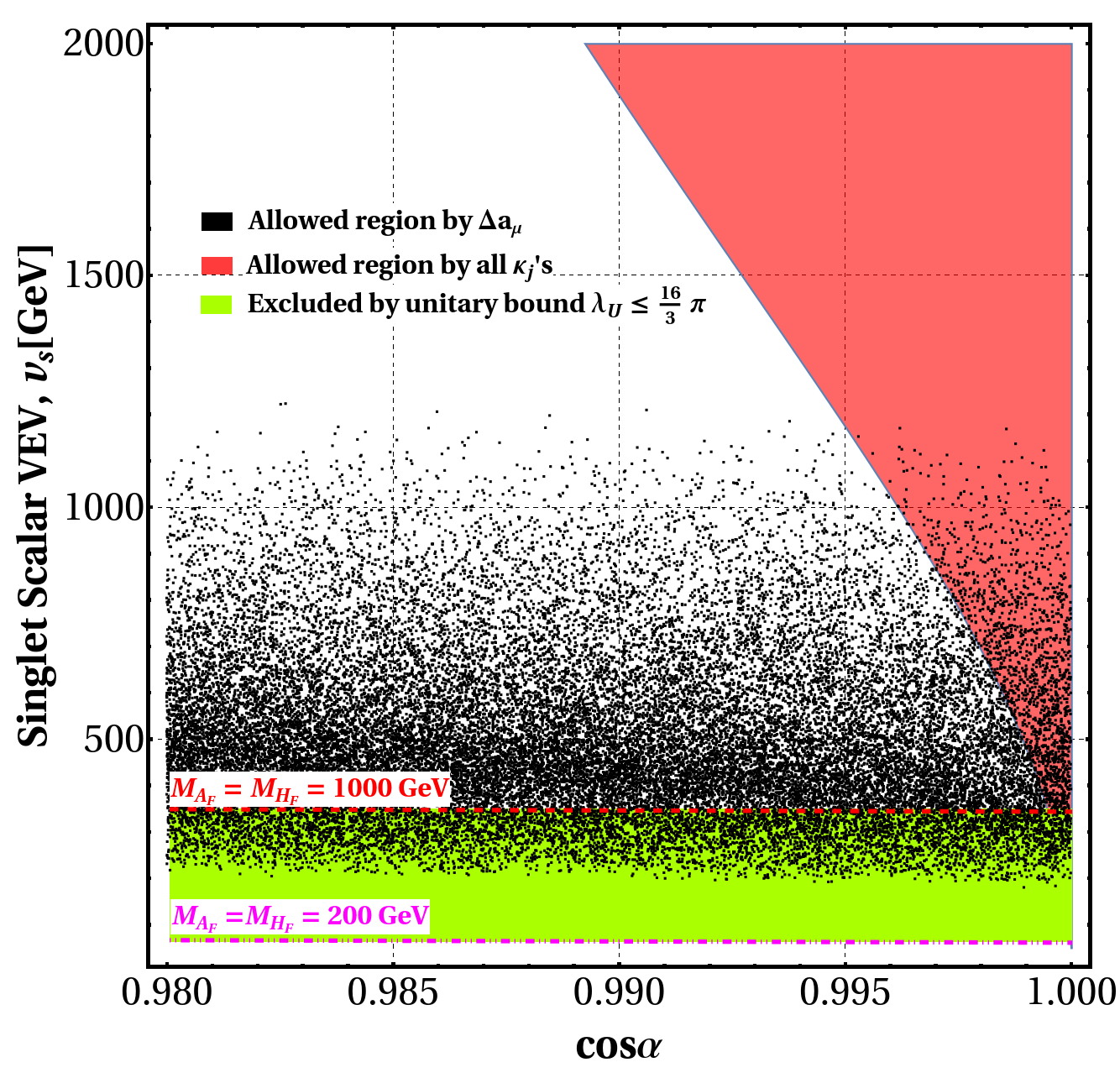
Furthermore, we present in Fig. 3 the $\cos\alpha-v_{s}$ plane regions allowed by $\Delta a_{\mu}$ (black points), $\Delta a_{e}$ (magenta points), $\mu\to 3e$ (red points) and $B_{s}^{0}\to\mu^{+}\mu^{-}$ (blue area). We have also analyzed the decays $\tau\to 3\mu$, $\tau\to\mu\gamma$, $\mu\to\ e\gamma$, however, these processes are not very restrictive in the FNSM. This is mainly due to the choice we made for the matrix elements $\tilde{Z}_{\mu\mu}$ and $\tilde{Z}_{\tau\tau}$, as they play a subtle role in the couplings (see Tab. 1) $\phi\mu^{-}\mu^{+}$ and $\phi\tau^{-}\tau^{+}$ ($\phi=h,\,H_{F},\,A_{F}$), which have a significant impact on the observables $\tau\to 3\mu$, $\tau\to\mu\gamma$, $\mu\to\ e\gamma$. In fact, we use $\tilde{Z}_{\tau\tau}=0.2$ and $\tilde{Z}_{\mu\mu}=10^{-4}$ (hence, a strong hierarchy), otherwise the SM $h\mu^{-}\mu^{+}$ coupling would be swamped by new corrections due to the FNSM¹¹ 1 Such a choice was adopted in the evaluation of $\kappa_{\tau\tau}$ and $\kappa_{\mu\mu}$, respectively, and then we scanned on the $\cos\alpha-v_{s}$ plane, as shown in Fig. 3.. So the bounds coming from the processes $\tau\to 3\mu$, $\tau\to\mu\gamma$, $\mu\to\ e\gamma$ are not included in Fig. 3.

Then, in Fig. 4, we display the result of applying all discussed theoretical and experimental constraints, limitedly to the reduced interval $0.98\leq\cos\alpha\leq 1$, since it is the region in which all the analyzed observables converge. Here, we only show the most restrictive bounds so as to not overload the plot. Among the latter, the unitarity bound plays a special role, as it helped us to find a lower limit for the singlet scalar VEV, $v_{s}$, depending on the Flavon mass, e.g., for $M_{H_{F}}=1000$ GeV one has $v_{s}\geq 345$ GeV. By comparison, the intersection of all $\kappa_{i}$’s and $\Delta a_{\mu}$ imposes a less stringent upper limit of $v_{s}\leq 1200$ GeV²² 2 Notice that, to generate Figs. 3, 3 and 4, we have used our own Mathematica package, so-called SpaceMath Arroyo-Urena:2020qup, which is available upon request..

As far as the CP-even Flavon mass $M_{H_{F}}$ is concerned, to constrain it, we use the limit on the cross section of the process $pp\to\phi\to hh$ from CMS:2018ipl, in which a combination of searches for SM-like Higgs boson pair production in proton-proton collisions at $\sqrt{s}=$13 TeV and 35.9 fb^-1 is reported. We present in Fig. 5 the cross section of the process $\sigma(pp\to H_{F}\to hh)$ in the FNSM as a function of $M_{H_{F}}$ and its comparison with the limit on $\sigma(pp\to\Phi\to hh)$, where $\phi$ stands for a generic spin-0 resonance. Furthermore, we show in Figs. 6 and 6 a comparison between the FNSM predictions and the ATLAS Collaboration limits atlas, now for individual channels with final states $b\bar{b}b\bar{b}$ and $b\bar{b}\tau^{-}\tau^{+}$, respectively. The most stringent constraints ATLAS:2021ifb come from $b\bar{b}\gamma\gamma$ production channel as shown in Fig. 7. In obtaining such limits, we have evaluated the inclusive cross section of our signal process, wherein we have used $v_{s}=1000$ GeV ans $\cos\alpha=0.995$. It is observed that the $M_{H_{F}}=300-1000$ GeV interval satisfies the bounds imposed, so we will define Benchmark Points (BPs) with $H_{F}$ masses herein. The model parameter space in this analysis is also consistent from the other search channels $pp\to H_{F}\to ZZ$ at ATLAS ATLAS:2020tlo and $pp\to H_{F}\to WW$ at CMS CMS:2019bnu.

Finally, because the $g_{H_{F}tc}$ coupling is proportional to the $\tilde{Z}_{tc}$ matrix element, we need a bound on it in order to evaluate the $H_{F}\to tc$ decay. Currently, there no specific processes that provide a stringent limit $\tilde{Z}_{tc}$, but we can estimate its order of magnitude by considering the upper limit on the Branching Ratio (BR) of $t\to ch$ at $<1.1\times 10^{-3}$ Workman:2022ynf. We also consider the prospects for ${\rm BR}(t\to ch)<4.3\times 10^{-5}$ searches at the FCC-hh Mandrik:2018yhe. The resulting allowed region in the $v_{s}-\tilde{Z}_{tc}$ plane is illustrated in Fig. 8. It is worth noting here that the behavior of the $\tilde{Z}_{tc}$ matrix element shows an increasing (decreasing) trend as $v_{s}$ increases (decreases). This observation is expected since the $g_{htc}$ coupling is governed by $\tilde{Z}_{tc}/v_{s}$. In order to have a realistic evaluation of the observables studied here, we adopt conservative values for $\tilde{Z}_{tc}$ and $v_{s}$.

The major SM backgrounds typically have the form $hh+X$ (where $X$ is known SM particles), which includes SM Higgs pair $hh$ production, $h+X$ like $hZ,hb\bar{b}$ and $ht\bar{t}$, as well as the non-Higgs processes which include $t\bar{t}$ and $t\bar{t}\gamma$ (here, leptons may fake as photons) as well as $b\bar{b}\gamma\gamma$, $c\bar{c}\gamma\gamma$ and $jj\gamma\gamma$ (where $c$-jets and light-jets may fake $b$-jets). The other relevant reducible backgrounds comprise $b\bar{b}j\gamma,c\bar{c}j\gamma$ and $b\bar{b}jj$, where $c$-jets may appear as $b$-jets and a light-jet may fake a photon. The fake rate of a light-jet $j$ into a photon depends on the momentum of the jet, $p_{T}^{j}$ ATLAS:2013kpx, as $9.3\times 10^{-3}{\rm exp}(-p_{T}^{j}/27.5~{\rm GeV})$. The $c$-jet is misidentified as a $b$-jet with a rate of $3.5\%$ whereas a light-jet mimics a $b$-jet with a rate of $0.135\%$ CMS:2017wtu.

We next present a detailed discussion of the collider search strategy employed to maximize the signal significance in the search channel $pp\to H_{F}\to hh~(h\to\gamma\gamma,h\to b\bar{b})$. To start with, though, we show the production and decay cross section $pp\to H_{F}\to hh~(h\to\gamma\gamma,h\to b\bar{b})$ for the three BPs presented in Tab. 2 (with, in particular, $M_{H_{F}}=800,~900$ and $1000$ GeV, as seen in Tab. 3). The corresponding dominant SM backgrounds are shown in Tab. 4.

Any charged objects (leptons or jets) or photons produced in any hard scattering process at the LHC will be observed in the detector if and only if they satisfy certain geometric criteria, known as acceptance cuts. These are the same for both the signal and background events and reproduce the accessible region of the detector. We will then have to ask that both signal and background events pass these acceptance cuts, which are, in general, not sufficient to separate the two samples. However, eventually, we will construct various kinematic observables and study their distributions. Next, we will decide the final selection cuts after studying the distinguishing features of those distributions between signal and backgrounds, so as to increase the former and decrease the latter. We base this approach on a Monte Carlo (MC) analysis using the tools previously described.

In our current scenario, an event is required to have exactly two $b$-tagged jets and two isolated photons $(\gamma)$ in the final state. However, we do not put any constraints on the number of light-jets. We then adopt the following acceptance cuts:

• •

  $p_{T}^{\gamma}>20$ GeV;

• •

  $p_{T}^{e/\mu}>20$ GeV (if an electron/muon is present, for $b$-tagging purposes);

• •

  $p_{T}^{j}>40$ GeV, where $j$ stands for light-jets as well as $b$-jets;

• •

  $\mid\eta_{\ell}\mid~\leq 2.5$ (again, $\ell=e/\mu$), $\mid\eta_{\gamma}\mid~\leq 2.0$ and $\mid\eta_{j}\mid~\leq 2.0$.

After considering these basic requirements, we apply a stronger selection (using additional kinematic variables) in order to enhance the signal-to-background ratio, as explained. A variety of such observables have been used to design the optimized Signal Region (SR), i.e., where the significance is maximized. First and foremost, the transverse momentum of photons ($p_{T}^{\gamma_{1}}$, $p_{T}^{\gamma_{2}}$) and $b$-jets ($p_{T}^{b_{1}}$, $p_{T}^{b_{2}}$)³³ 3 Here, ${1}$ and ${2}$ represents the $p_{T}$ ordered leading and sub-leading photon and $b$-jet in the final state. will be studied. In addition, the separation between the two final state photons $\Delta R_{\gamma_{1}\gamma_{2}}$ and $b$-jets $\Delta R_{b_{1}b_{2}}$ are also used. The separation between two detector objects, $\Delta R$, is defined as $\Delta R=\sqrt{\Delta\eta^{2}+\Delta\phi^{2}}$, where $\Delta\eta$ and $\Delta\phi$ are the differences in pseudorapidity and azimuthal angle, respectively. Then, the invariant mass of the final state photons ($M_{\gamma_{1}\gamma_{2}}$) and $b$-jets ($M_{b_{1}b_{2}}$) will also be used to discriminate between signal and backgrounds, where we have introduced $M_{ab}=\sqrt{(E^{a}+E^{b})^{2}-\sum_{i=x,y,x}(p_{i}^{a}+p_{i}^{b})^{2}}$, with $ab=\gamma_{1}\gamma_{2}$ or $b_{1}b_{2}$. Finally, we use the invariant mass $M_{hh}$ for the final extraction. The $M_{hh}$ variable has been calculated as $M_{hh}=\sqrt{(E^{\gamma_{1}}+E^{\gamma_{2}}+E^{b_{1}}+E^{b_{2}})^{2}-\sum_{i=x,y,z}(p^{\gamma_{1}}_{i}+p^{\gamma_{2}}_{i}+p^{b_{1}}_{i}+p^{b_{2}}_{i})^{2}}.$ In the above formulae, $E$ and $p_{i}~(i=x,y,z)$ stand for the energy and three-momentum component of the final state particles, respectively.

References

- (1) ATLAS Collaboration, G. Aad et al., “Observation of a new particle in the search for the Standard Model Higgs boson with the ATLAS detector at the LHC,” Phys. Lett. B 716 (2012) 1–29, arXiv:1207.7214 [hep-ex].
- (2) CMS Collaboration, S. Chatrchyan et al., “Observation of a New Boson at a Mass of 125 GeV with the CMS Experiment at the LHC,” Phys. Lett. B 716 (2012) 30–61, arXiv:1207.7235 [hep-ex].
- (3) P. P. Giardino, K. Kannike, I. Masina, M. Raidal, and A. Strumia, “The universal Higgs fit,” JHEP 05 (2014) 046, arXiv:1303.3570 [hep-ph].
- (4) CMS Collaboration, A. M. Sirunyan et al., “Observation of the Higgs boson decay to a pair of leptons with the CMS detector,” Phys. Lett. B779 (2018) 283–316, arXiv:1708.00373 [hep-ex].
- (5) CMS Collaboration, A. M. Sirunyan et al., “Combined measurements of Higgs boson couplings in proton–proton collisions at ,” Eur. Phys. J. C79 no. 5, (2019) 421, arXiv:1809.10733 [hep-ex].
- (6) Z. Kunszt, S. Moretti, and W. J. Stirling, “Higgs production at the LHC: An Update on cross-sections and branching ratios,” Z. Phys. C 74 (1997) 479–491, arXiv:hep-ph/9611397.
- (7) S. Dawson, S. Dittmaier, and M. Spira, “Neutral Higgs boson pair production at hadron colliders: QCD corrections,” Phys. Rev. D 58 (1998) 115012, arXiv:hep-ph/9805244.
- (8) J. Baglio, F. Campanario, S. Glaus, M. Mühlleitner, M. Spira, and J. Streicher, “Gluon fusion into Higgs pairs at NLO QCD and the top mass scheme,” Eur. Phys. J. C 79 no. 6, (2019) 459, arXiv:1811.05692 [hep-ph].
- (9) J. Baglio, F. Campanario, S. Glaus, M. Mühlleitner, J. Ronca, M. Spira, and J. Streicher, “Higgs-Pair Production via Gluon Fusion at Hadron Colliders: NLO QCD Corrections,” JHEP 04 (2020) 181, arXiv:2003.03227 [hep-ph].
- (10) ATLAS Collaboration, M. Aaboud et al., “Search for heavy ZZ resonances in the and final states using proton–proton collisions at TeV with the ATLAS detector,” Eur. Phys. J. C 78 no. 4, (2018) 293, arXiv:1712.06386 [hep-ex].
- (11) J. Baglio, L. D. Ninh, and M. M. Weber, “Massive gauge boson pair production at the LHC: a next-to-leading order story,” Phys. Rev. D 88 (2013) 113005, arXiv:1307.4331 [hep-ph]. [Erratum: Phys.Rev.D 94, 099902 (2016)].
- (12) A. Adhikary, S. Banerjee, R. K. Barman, B. Bhattacherjee, and S. Niyogi, “Revisiting the non-resonant Higgs pair production at the HL-LHC,” JHEP 07 (2018) 116, arXiv:1712.05346 [hep-ph].
- (13) ATLAS Collaboration, G. Aad et al., “Search for heavy resonances decaying into a pair of Z bosons in the and final states using 139 of proton–proton collisions at TeV with the ATLAS detector,” Eur. Phys. J. C 81 no. 4, (2021) 332, arXiv:2009.14791 [hep-ex].
- (14) J. Baglio, A. Djouadi, R. Gröber, M. M. Mühlleitner, J. Quevillon, and M. Spira, “The measurement of the Higgs self-coupling at the LHC: theoretical status,” JHEP 04 (2013) 151, arXiv:1212.5581 [hep-ph].
- (15) V. Barger, L. L. Everett, C. B. Jackson, and G. Shaughnessy, “Higgs-Pair Production and Measurement of the Triscalar Coupling at LHC(8,14),” Phys. Lett. B 728 (2014) 433–436, arXiv:1311.2931 [hep-ph].
- (16) N. Kumar and S. P. Martin, “LHC search for di-Higgs decays of stoponium and other scalars in events with two photons and two bottom jets,” Phys. Rev. D 90 no. 5, (2014) 055007, arXiv:1404.0996 [hep-ph].
- (17) A. Adhikary, S. Banerjee, R. Kumar Barman, and B. Bhattacherjee, “Resonant heavy Higgs searches at the HL-LHC,” JHEP 09 (2019) 068, arXiv:1812.05640 [hep-ph].
- (18) A. Adhikary, R. K. Barman, and B. Bhattacherjee, “Prospects of non-resonant di-Higgs searches and Higgs boson self-coupling measurement at the HE-LHC using machine learning techniques,” JHEP 12 (2020) 179, arXiv:2006.11879 [hep-ph].
- (19) J. Baglio, O. Eberhardt, U. Nierste, and M. Wiebusch, “Benchmarks for Higgs Pair Production and Heavy Higgs boson Searches in the Two-Higgs-Doublet Model of Type II,” Phys. Rev. D 90 no. 1, (2014) 015008, arXiv:1403.1264 [hep-ph].
- (20) B. Hespel, D. Lopez-Val, and E. Vryonidou, “Higgs pair production via gluon fusion in the Two-Higgs-Doublet Model,” JHEP 09 (2014) 124, arXiv:1407.0281 [hep-ph].
- (21) L.-C. Lü, C. Du, Y. Fang, H.-J. He, and H. Zhang, “Searching heavier Higgs boson via di-Higgs production at LHC Run-2,” Phys. Lett. B 755 (2016) 509–522, arXiv:1507.02644 [hep-ph].
- (22) G. D. Kribs and A. Martin, “Enhanced di-Higgs Production through Light Colored Scalars,” Phys. Rev. D 86 (2012) 095023, arXiv:1207.4496 [hep-ph].
- (23) L. Bian and N. Chen, “Higgs pair productions in the CP-violating two-Higgs-doublet model,” JHEP 09 (2016) 069, arXiv:1607.02703 [hep-ph].
- (24) S. Dawson, E. Furlan, and I. Lewis, “Unravelling an extended quark sector through multiple Higgs production?,” Phys. Rev. D 87 no. 1, (2013) 014007, arXiv:1210.6663 [hep-ph].
- (25) A. Pierce, J. Thaler, and L.-T. Wang, “Disentangling Dimension Six Operators through Di-Higgs Boson Production,” JHEP 05 (2007) 070, arXiv:hep-ph/0609049.
- (26) S. Kanemura and K. Tsumura, “Effects of the anomalous Higgs couplings on the Higgs boson production at the Large Hadron Collider,” Eur. Phys. J. C 63 (2009) 11–21, arXiv:0810.0433 [hep-ph].
- (27) U. Ellwanger, “Higgs pair production in the NMSSM at the LHC,” JHEP 08 (2013) 077, arXiv:1306.5541 [hep-ph].
- (28) C.-R. Chen and I. Low, “Double take on new physics in double Higgs boson production,” Phys. Rev. D 90 no. 1, (2014) 013018, arXiv:1405.7040 [hep-ph].
- (29) N. Liu, S. Hu, B. Yang, and J. Han, “Impact of top-Higgs couplings on Di-Higgs production at future colliders,” JHEP 01 (2015) 008, arXiv:1408.4191 [hep-ph].
- (30) F. Goertz, A. Papaefstathiou, L. L. Yang, and J. Zurita, “Higgs boson pair production in the D=6 extension of the SM,” JHEP 04 (2015) 167, arXiv:1410.3471 [hep-ph].
- (31) A. Azatov, R. Contino, G. Panico, and M. Son, “Effective field theory analysis of double Higgs boson production via gluon fusion,” Phys. Rev. D 92 no. 3, (2015) 035001, arXiv:1502.00539 [hep-ph].
- (32) M. J. Dolan, C. Englert, and M. Spannowsky, “New Physics in LHC Higgs boson pair production,” Phys. Rev. D 87 no. 5, (2013) 055002, arXiv:1210.8166 [hep-ph].
- (33) V. Barger, L. L. Everett, C. B. Jackson, A. D. Peterson, and G. Shaughnessy, “New physics in resonant production of Higgs boson pairs,” Phys. Rev. Lett. 114 no. 1, (2015) 011801, arXiv:1408.0003 [hep-ph].
- (34) A. Crivellin, M. Ghezzi, and M. Procura, “Effective Field Theory with Two Higgs Doublets,” JHEP 09 (2016) 160, arXiv:1608.00975 [hep-ph].
- (35) H. Sun, Y.-J. Zhou, and H. Chen, “Constraints on large-extra-dimensions model through 125-GeV Higgs pair production at the LHC,” Eur. Phys. J. C 72 (2012) 2011, arXiv:1211.5197 [hep-ph].
- (36) R. Costa, M. Mühlleitner, M. O. P. Sampaio, and R. Santos, “Singlet Extensions of the Standard Model at LHC Run 2: Benchmarks and Comparison with the NMSSM,” JHEP 06 (2016) 034, arXiv:1512.05355 [hep-ph].
- (37) K. Cheung, A. Jueid, C.-T. Lu, J. Song, and Y. W. Yoon, “Disentangling new physics effects on nonresonant Higgs boson pair production from gluon fusion,” Phys. Rev. D 103 no. 1, (2021) 015019, arXiv:2003.11043 [hep-ph].
- (38) A. Alves, D. Gonçalves, T. Ghosh, H.-K. Guo, and K. Sinha, “Di-Higgs Production in the Channel and Gravitational Wave Complementarity,” JHEP 03 (2020) 053, arXiv:1909.05268 [hep-ph].
- (39) C. Englert and J. Jaeckel, “Probing the Symmetric Higgs Portal with Di-Higgs Boson Production,” Phys. Rev. D 100 no. 9, (2019) 095017, arXiv:1908.10615 [hep-ph].
- (40) P. Basler, S. Dawson, C. Englert, and M. Mühlleitner, “Showcasing HH production: Benchmarks for the LHC and HL-LHC,” Phys. Rev. D 99 no. 5, (2019) 055048, arXiv:1812.03542 [hep-ph].
- (41) Z. Heng, X. Gong, and H. Zhou, “Pair production of Higgs boson in NMSSM at the LHC with the next-to-lightest CP-even Higgs boson being SM-like,” Chin. Phys. C 42 no. 7, (2018) 073103, arXiv:1805.01598 [hep-ph].
- (42) B. Das, S. Moretti, S. Munir, and P. Poulose, “Quantum interference effects in Higgs boson pair-production beyond the Standard Model,” Eur. Phys. J. C 81 no. 4, (2021) 347, arXiv:2012.09587 [hep-ph].
- (43) H. Abouabid, A. Arhrib, D. Azevedo, J. E. Falaki, P. M. Ferreira, M. Mühlleitner, and R. Santos, “Benchmarking Di-Higgs Production in Various Extended Higgs Sector Models,” arXiv:2112.12515 [hep-ph].
- (44) S. Dasgupta, R. Pramanick, and T. S. Ray, “Broad toplike vector quarks at LHC and HL-LHC,” Phys. Rev. D 105 no. 3, (2022) 035032, arXiv:2112.03742 [hep-ph].
- (45) L. Huang, S.-b. Kang, J. H. Kim, K. Kong, and J. S. Pi, “Portraying Double Higgs at the Large Hadron Collider II,” arXiv:2203.11951 [hep-ph].
- (46) G. Li, L.-X. Xu, B. Yan, and C. P. Yuan, “Resolving the degeneracy in top quark Yukawa coupling with Higgs pair production,” Phys. Lett. B 800 135070, arXiv:1904.12006 [hep-ph].
- (47) Q.-H. Cao, B. Yan, D.-M. Zhang, and H. Zhang, “Resolving the Degeneracy in Single Higgs Production with Higgs Pair Production,” Phys. Lett. B 752 (2016) 285–290, arXiv:1508.06512 [hep-ph].
- (48) Q.-H. Cao, G. Li, B. Yan, D.-M. Zhang, and H. Zhang, “Double Higgs production at the 14 TeV LHC and a 100 TeV collider,” Phys. Rev. D 96 no. 9, 095031, arXiv:1611.09336 [hep-ph].
- (49) J. Cao, D. Li, L. Shang, P. Wu, and Y. Zhang, “Exploring the Higgs Sector of a Most Natural NMSSM and its Prediction on Higgs Pair Production at the LHC,” JHEP 12 (2014) 026, arXiv:1409.8431 [hep-ph].
- (50) J. Cao, Z. Heng, L. Shang, P. Wan, and J. M. Yang, “Pair Production of a 125 GeV Higgs Boson in MSSM and NMSSM at the LHC,” JHEP 04 (2013) 134, arXiv:1301.6437 [hep-ph].
- (51) C.-T. Lu, J. Chang, K. Cheung, and J. S. Lee, “An exploratory study of Higgs-boson pair production,” JHEP 08 (2015) 133, arXiv:1505.00957 [hep-ph].
- (52) J. Kopp, “Flavor Violation in the Scalar Sector,” in 51st Rencontres de Moriond on EW Interactions and Unified Theories, pp. 281–288. 2016. arXiv:1605.02865 [hep-ph].
- (53) E. Arganda, X. Marcano, N. I. Mileo, R. A. Morales, and A. Szynkman, “Model-independent search strategy for the lepton-flavor-violating heavy Higgs boson decay to at the LHC,” Eur. Phys. J. C 79 no. 9, (2019) 738, arXiv:1906.08282 [hep-ph].
- (54) B. Altunkaynak, W.-S. Hou, C. Kao, M. Kohda, and B. McCoy, “Flavor Changing Heavy Higgs Interactions at the LHC,” Phys. Lett. B 751 (2015) 135–142, arXiv:1506.00651 [hep-ph].
- (55) I. Doršner, S. Fajfer, A. Greljo, J. F. Kamenik, and N. Košnik, “Physics of leptoquarks in precision experiments and at particle colliders,” Phys. Rept. 641 (2016) 1–68, arXiv:1603.04993 [hep-ph].
- (56) A. Davidson, V. P. Nair, and K. C. Wali, “Peccei-Quinn Symmetry as Flavor Symmetry and Grand Unification,” Phys. Rev. D 29 (1984) 1504.
- (57) A. Davidson and K. C. Wali, “MINIMAL FLAVOR UNIFICATION VIA MULTIGENERATIONAL PECCEI-QUINN SYMMETRY,” Phys. Rev. Lett. 48 (1982) 11.
- (58) C. D. Froggatt and H. B. Nielsen, “Hierarchy of Quark Masses, Cabibbo Angles and CP Violation,” Nucl. Phys. B 147 (1979) 277–298.
- (59) A. Bolaños, J. L. Diaz-Cruz, G. Hernández-Tomé, and G. Tavares-Velasco, “Has a Higgs-flavon with a GeV mass been detected at the LHC13?,” Phys. Lett. B 761 (2016) 310–317, arXiv:1604.04822 [hep-ph].
- (60) M. Bauer, T. Schell, and T. Plehn, “Hunting the Flavon,” Phys. Rev. D 94 no. 5, (2016) 056003, arXiv:1603.06950 [hep-ph].
- (61) K. Huitu, V. Keus, N. Koivunen, and O. Lebedev, “Higgs-flavon mixing and ,” JHEP 05 (2016) 026, arXiv:1603.06614 [hep-ph].
- (62) E. L. Berger, S. B. Giddings, H. Wang, and H. Zhang, “Higgs-flavon mixing and LHC phenomenology in a simplified model of broken flavor symmetry,” Phys. Rev. D 90 no. 7, (2014) 076004, arXiv:1406.6054 [hep-ph].
- (63) J. L. Diaz-Cruz and U. J. Saldaña Salazar, “Higgs couplings and new signals from Flavon–Higgs mixing effects within multi-scalar models,” Nucl. Phys. B 913 (2016) 942–963, arXiv:1405.0990 [hep-ph].
- (64) M. A. Arroyo-Ureña, J. L. Díaz-Cruz, G. Tavares-Velasco, A. Bolaños, and G. Hernández-Tomé, “Searching for lepton flavor violating flavon decays at hadron colliders,” Phys. Rev. D 98 no. 1, (2018) 015008, arXiv:1801.00839 [hep-ph].
- (65) M. A. Arroyo-Ureña, A. Fernández-Téllez, and G. Tavares-Velasco, “Flavor changing flavon decay at the high luminosity large hadron collider,” Rev. Mex. Fis. 69 no. 2, (2023) 020803, arXiv:1906.07821 [hep-ph].
- (66) K. Tsumura and L. Velasco-Sevilla, “Phenomenology of flavon fields at the LHC,” Phys. Rev. D 81 (2010) 036012, arXiv:0911.2149 [hep-ph].
- (67) F. Gianotti et al., “Physics potential and experimental challenges of the LHC luminosity upgrade,” Eur. Phys. J. C 39 (2005) 293–333, arXiv:hep-ph/0204087.
- (68) G. Apollinari, O. Brüning, T. Nakamoto, and L. Rossi, “High Luminosity Large Hadron Collider HL-LHC,” CERN Yellow Rep. no. 5, (2015) 1–19, arXiv:1705.08830 [physics.acc-ph].
- (69) ATLAS Collaboration, G. Aad et al., “Combination of searches for Higgs boson pairs in collisions at 13 TeV with the ATLAS detector,” Phys. Lett. B 800 (2020) 135103, arXiv:1906.02025 [hep-ex].
- (70) ATLAS Collaboration, M. Aaboud et al., “Search for Higgs boson pair production in the decay channel using ATLAS data recorded at TeV,” JHEP 05 (2019) 124, arXiv:1811.11028 [hep-ex].
- (71) ATLAS Collaboration, M. Aaboud et al., “Search for Higgs boson pair production in the decay mode at TeV with the ATLAS detector,” JHEP 04 (2019) 092, arXiv:1811.04671 [hep-ex].
- (72) ATLAS Collaboration, M. Aaboud et al., “Search for resonant and non-resonant Higgs boson pair production in the decay channel in collisions at TeV with the ATLAS detector,” Phys. Rev. Lett. 121 no. 19, (2018) 191801, arXiv:1808.00336 [hep-ex]. [Erratum: Phys.Rev.Lett. 122, 089901 (2019)].
- (73) CMS Collaboration, A. M. Sirunyan et al., “Search for Higgs boson pair production in events with two bottom quarks and two tau leptons in proton–proton collisions at =13TeV,” Phys. Lett. B 778 (2018) 101–127, arXiv:1707.02909 [hep-ex].
- (74) ATLAS Collaboration, M. Aaboud et al., “Search for Higgs boson pair production in the channel using collision data recorded at TeV with the ATLAS detector,” Eur. Phys. J. C 78 no. 12, (2018) 1007, arXiv:1807.08567 [hep-ex].
- (75) ATLAS Collaboration, M. Aaboud et al., “Search for Higgs boson pair production in the final state with 13 TeV collision data collected by the ATLAS experiment,” JHEP 11 (2018) 040, arXiv:1807.04873 [hep-ex].
- (76) ATLAS Collaboration, M. Aaboud et al., “Search for pair production of Higgs bosons in the final state using proton-proton collisions at TeV with the ATLAS detector,” JHEP 01 (2019) 030, arXiv:1804.06174 [hep-ex].
- (77) CMS Collaboration, A. M. Sirunyan et al., “Combination of searches for Higgs boson pair production in proton-proton collisions at 13 TeV,” Phys. Rev. Lett. 122 no. 12, (2019) 121803, arXiv:1811.09689 [hep-ex].
- (78) ATLAS Collaboration, “Constraints on the Higgs boson self-coupling from the combination of single-Higgs and double-Higgs production analyses performed with the ATLAS experiment,”.
- (79) ATLAS Collaboration, “Measurement and interpretation of same-sign boson pair production in association with two jets in collisions at TeV with the ATLAS detector,”.
- (80) ATLAS Collaboration, G. Aad et al., “Evidence of off-shell Higgs boson production from leptonic decay channels and constraints on its total width with the ATLAS detector,” arXiv:2304.01532 [hep-ex].
- (81) D. Zubov, D. Pyatiizbyantseva, and E. Soldatov, “An Improved Selection Optimization Method Used for the Measurement of Production under Conditions of ATLAS Experiment during LHC Run II,” Phys. Part. Nucl. 54 no. 1, (2023) 232–238.
- (82) C. Bonilla, D. Sokolowska, N. Darvishi, J. L. Diaz-Cruz, and M. Krawczyk, “IDMS: Inert Dark Matter Model with a complex singlet,” J. Phys. G 43 no. 6, (2016) 065001, arXiv:1412.8730 [hep-ph].
- (83) E. Barradas-Guevara, J. L. Diaz-Cruz, O. Félix-Beltrán, and U. J. Saldana-Salazar, “Linking LFV Higgs decays with CP violation in multi-scalar models,” arXiv:1706.00054 [hep-ph].
- (84) N. Khan and S. Rakshit, “Study of electroweak vacuum metastability with a singlet scalar dark matter,” Phys. Rev. D 90 no. 11, (2014) 113008, arXiv:1407.6015 [hep-ph].
- (85) G. Cynolter, E. Lendvai, and G. Pocsik, “Note on unitarity constraints in a model for a singlet scalar dark matter candidate,” Acta Phys. Polon. B 36 (2005) 827–832, arXiv:hep-ph/0410102.
- (86) M. Cepeda et al., “Report from Working Group 2: Higgs Physics at the HL-LHC and HE-LHC,” CERN Yellow Rep. Monogr. 7 (2019) 221–584, arXiv:1902.00134 [hep-ph].
- (87) M. A. Arroyo-Ureña, R. Gaitán, and T. A. Valencia-Pérez, “SpaceMath version 1.0 A Mathematica package for beyond the standard model parameter space searches,” Rev. Mex. Fis. E 19 no. 2, (2022) 020206, arXiv:2008.00564 [hep-ph].
- (88) “Search for elusive ”di-higgs production” reaches new milestone.” https://atlas.cern/updates/briefing/new-milestone-di-Higgs-search.
- (89) ATLAS Collaboration, G. Aad et al., “Search for Higgs boson pair production in the two bottom quarks plus two photons final state in collisions at TeV with the ATLAS detector,” Phys. Rev. D 106 no. 5, (2022) 052001, arXiv:2112.11876 [hep-ex].
- (90) CMS Collaboration, A. M. Sirunyan et al., “Search for a heavy Higgs boson decaying to a pair of W bosons in proton-proton collisions at 13 TeV,” JHEP 03 (2020) 034, arXiv:1912.01594 [hep-ex].
- (91) Particle Data Group Collaboration, R. L. Workman et al., “Review of Particle Physics,” PTEP 2022 (2022) 083C01.
- (92) FCC Study Group Collaboration, P. Mandrik, “Prospect for top quark FCNC searches at the FCC-hh,” J. Phys. Conf. Ser. 1390 no. 1, (2019) 012044, arXiv:1812.00902 [hep-ex].
- (93) A. Alloul, N. D. Christensen, C. Degrande, C. Duhr, and B. Fuks, “FeynRules 2.0 - A complete toolbox for tree-level phenomenology,” Comput. Phys. Commun. 185 (2014) 2250–2300, arXiv:1310.1921 [hep-ph].
- (94) J. Alwall, R. Frederix, S. Frixione, V. Hirschi, F. Maltoni, O. Mattelaer, H. S. Shao, T. Stelzer, P. Torrielli, and M. Zaro, “The automated computation of tree-level and next-to-leading order differential cross sections, and their matching to parton shower simulations,” JHEP 07 (2014) 079, arXiv:1405.0301 [hep-ph].
- (95) T. Sjöstrand, S. Ask, J. R. Christiansen, R. Corke, N. Desai, P. Ilten, S. Mrenna, S. Prestel, C. O. Rasmussen, and P. Z. Skands, “An introduction to PYTHIA 8.2,” Comput. Phys. Commun. 191 (2015) 159–177, arXiv:1410.3012 [hep-ph].
- (96) DELPHES 3 Collaboration, J. de Favereau, C. Delaere, P. Demin, A. Giammanco, V. Lemaître, A. Mertens, and M. Selvaggi, “DELPHES 3, A modular framework for fast simulation of a generic collider experiment,” JHEP 02 (2014) 057, arXiv:1307.6346 [hep-ex].
- (97) T. Plehn, “Lectures on LHC Physics,” Lect. Notes Phys. 844 (2012) 1–193, arXiv:0910.4182 [hep-ph].
- (98) ATLAS Collaboration, “Performance assumptions based on full simulation for an upgraded ATLAS detector at a High-Luminosity LHC,” ATL-PHYS-PUB-2013-009 (2013) .
- (99) CMS Collaboration, A. M. Sirunyan et al., “Identification of heavy-flavour jets with the CMS detector in pp collisions at 13 TeV,” JINST 13 no. 05, (2018) P05011, arXiv:1712.07158 [physics.ins-det].
- (100) G. Cowan, “Discovery sensitivity for a counting experiment with background uncertainty,” Technical report, Royal Holloway (U.K) University of London.