El-WaveHoltz: A Time-Domain Iterative Solver for Time-Harmonic Elastic Waves
Abstract
We consider the application of the WaveHoltz iteration to time-harmonic elastic wave equations with energy conserving boundary conditions. The original WaveHoltz iteration for acoustic Helmholtz problems is a fixed-point iteration that filters the solution of the wave equation with time-harmonic forcing and boundary data. As in the original WaveHoltz method, we reformulate the fixed point iteration as a positive definite linear system of equations that is iteratively solved by a Krylov method. We present two time-stepping schemes, one explicit and one (novel) implicit, which completely remove time discretization error from the WaveHoltz solution by performing a simple modification of the initial data and time-stepping scheme. Numerical experiments indicate an iteration scaling similar to that of the original WaveHoltz method, and that the convergence rate is dictated by the shortest (shear) wave speed of the problem. We additionally show that the implicit scheme can be advantageous in practice for meshes with disparate element sizes.
Keywords:
Elastic wave equation , Helmholtz equation , Time-harmonic scattering1 Introduction
Time-harmonic wave propagation problems are notoriously difficult to solve by direct or iterative methods due to the resolution requirements and the indefinite nature of the differential operator, especially at high frequencies. For applications such as in solid mechanics, seismology and geophysics, we consider the time-harmonic elastic wave equation (or Navier equation 11 1 This is sometimes also referred to as the Navier-Cauchy equation, which is not to be confused with the ubiquitous Navier-Stokes equation.)
for a domain and frequency . Here is the density, is the displacement vector, the spatial dimension, is the stress tensor, and f is the forcing. Few effective solvers and preconditioners are available for the Navier equation, which are generally extensions of methods originally designed for the acoustic time-harmonic wave equation more commonly known as the Helmholtz equation. The efficient solution of the Helmholtz equation via iterative methods is an active area of research with a variety of methods in both the frequency and time-domain. We refer to our previous paper [3] for a more in-depth overview of the literature on techniques for solving the Helmholtz equation, as well as the review articles [21, 22, 20].
The elastic wave equation models both pressure and shear waves and, as is the case for the Helmholtz equation, the system of equations results in a discretization that is highly indefinite for large frequencies. As for any wave propagation problem the resolution must increase with the frequency, and here the most stringent resolution constraint comes from the (shorter) shear wave wavelength. This, in tandem with times the number of unknowns leading to larger storage requirements, necessitates parallel, memory lean, and scalable solvers that must be high order accurate to mitigate dispersive errors, [28], causing the so-called pollution effect [7].
While most methods have traditionally focused on solving the Helmholtz equation in the frequency domain (we provide a review of some of these below), an alternative approach is to instead construct iterative solvers in the time-domain. One such method, the so-called Controllability Method (CM), was first proposed by Bristeau et al. [12] and has recently received renewed interest in a series of papers by Grote et al.[25, 31, 15]. The CM was extended to elastic media in [32, 27]. The unknown in the CM is the initial data to the wave equation. In the CM this initial data is adjusted so that it produces an approximation to the Helmholtz equation by solving a constrained least-squares minimization where the objective function measures the deviation from time-periodicity. The minimization can be efficiently implemented using the conjugate gradient method, where the gradient is computed by solving the adjoint wave equation backwards in time.
It is possible, however, to find a time-harmonic wave equation solution by solving a single wave equation forward in time in each iteration. This can be done via the WaveHoltz method introduced in [3] for the scalar wave equation. We now provide an overview of the WaveHoltz method which was directly inspired by recent work on the CM, [25].
1.1 Overview of the El WaveHoltz Iteration
As in the CM, the WaveHoltz iteration (and the Elastic version we denote El WaveHoltz) iteratively updates the initial data to the wave equation. The marked difference between the two methods is that the WaveHoltz iteration updates the initial data by filtering the wave equation solution over one period (or an integer number of periods). The filtered solution is then used as the next initial data and thus the WaveHoltz method only requires one wave solve per iteration while the CM requires two.
In [3] we show that the (linear) iteration is convergent in both the continuous and discretized setting and that, if formulated as a linear system of equations, the underlying matrix is positive definite. We also showed that with energy conserving boundary conditions (Dirichlet or Neumann) the matrix is symmetric as long as the numerical method is symmetric (or symmetrizable).
We emphasize that the filter used in the WaveHoltz method corresponds to a bounded linear operator with an inverse that is also bounded. Therefore, the number of iterations (and the condition number of the problem) is essentially independent of the gridsize for well resolved grids. This is in contrast to methods that discretize and solve the PDE directly. Such methods typically have a condition number that scales as which makes it increasingly difficult to solve the problem as the solution becomes more accurate.
The analysis in [3] predicted that the WaveHoltz method in dimensions and accelerated by the conjugate gradient method converges to a fixed tolerance in iterations for energy conserving problems and numerical experiments indicated that it converges in iterations for open problems. The analytical predictions from [3] are expected to hold here as well and in the experiments we carry out below we observe . All these results and observations are independent of grid resolution indicating that our method can be particularly suitable when accurate solutions are required.
In this paper we focus solely on energy conserving boundary conditions (Dirichlet or normal stress) and leave the cases of impedance and non-reflecting boundary conditions to future work. In addition to introducing El WaveHoltz, we present several new results that are also retroactively applicable to our earlier work on WaveHoltz for the scalar wave equation [3] and Maxwell’s equations [33].
Following the ideas of Stolk [36] we introduce two new two-level time-stepping schemes – one explicit and one implicit – that remove the time-stepping error from the WaveHoltz solution. When either of these time-stepping methods are used the solution to the discrete WaveHoltz method is identical to the solution obtained by directly discretizing the frequency domain equation.
For high frequency, large scale problems, parallel solution of the Navier equation is the only feasible option. For a parallel solver to scale well the ratio of communication to computation should be small. In general, there are two types of communication: a) the local communications between processors to exchange local degrees of freedom needed for stencil operations in the discretization of spatial derivatives, and b) global all-to-all operations such as computing the inner product between two global vectors. The WaveHoltz method has an intrinsic advantage compared to methods that work directly with the frequency domain equation in that the all-to-all communication that is required to update search directions in CG, GMRES etc. only needs to be computed once per -period. Here we explore the effect of filtering over an additional number of periods to further reduce the number of all-to-all communications.
We believe that the method we propose here is an attractive alternative to previously proposed methods. In particular, El WaveHoltz is easily implemented if an elastic wave equation solver is already available. As we show in the numerical experiments section, El WaveHoltz can be one to two orders of magnitude faster compared to an algebraic multigrid (AMG) preconditioned GMRES solver for the frequency domain equation when using the symmetric interior penalty discontinuous Galerkin implementation available in MFEM [2]. There are, of course, many other solvers available; the question of which method will be most efficient will depend on the details of the problem to be solved. We now review some of the methods available in the literature.
1.2 Literature Review
One of the most common preconditioners for acoustic problems is the shifted Laplacian preconditioner (SLP), a more thorough review of which can be found in the review article by Erlangga [20]. One of the first extensions of the SLP to elastic media was introduced by Airaksinen et al. [1], in which a finite element spatial discretization for the preconditioned system is inverted by AMG. A more traditional finite difference multigrid SLP with line-relaxations was considered by Rizzuti and Mulder [34]. For both of these previous approaches, the effectiveness of a straightforward SLP is degraded for nearly incompressible media as the prolongation operators struggle to approximate the nullspace of the grad-div operator. To address this, a more recent extension was done by Treister [37] in which a mixed-formulation of the Navier equation is considered. While nearly incompressible media could be handled by the methods of [37], this comes at the cost of doubling the number of unknowns as well as additional storage requirements for precomputing the inverse of relaxation operators.
Another important class of methods for the solution of the Helmholtz equation are domain decomposition (DD) methods, for which we refer the reader to [22] for a review. In the short article [13], it was shown that a classic Schwarz DD with overlap for elastic problems converges for high frequencies, diverges for medium frequencies, and stagnates for small frequencies. Moreover, overlapping DD as a preconditioner for a GMRES accelerated solver exhibits convergence behavior that depends strongly on the frequency with degrading performance for increasing frequency. To remedy this, Brunet et al. introduced more general transmission conditions at the boundaries of overlapping domains in [14]. These transmission conditions, together with a sufficiently large enough overlap, yield convergence of the DD method for all frequencies with the exception of , where and are the shear and pressure wave speeds, respectively.
For unbounded problems one of the most promising classes of preconditioners for the Helmholtz equation are the so-called sweeping preconditioners by Engquist and Ying [18, 19]. These preconditioners construct an decomposition by sweeping through the domain layer-by-layer, with the key observation that the application of the Schur complement matrices found in the block diagonal matrix is equivalent to solving a quasi-1D(2D) problem in 2D(3D). In contrast to the acoustic case, however, the sweeping preconditioner for time-harmonic elastic waves, [38], exhibited an increase in the number of iterations with frequency for a heterogeneous media as the moving perfectly matched layer (PML) does not approximate Green’s function as well. We note that the stable construction of PML for many elastic problems is still considered an open question [10, 5]. Similar to the sweeping preconditioner, Belonosov et al. [11] construct a preconditioner in 3D with damping that sweeps through the domain along a coordinate axis while additionally homogenizing the medium in each layer. The preconditioner of [11] is inverted using FFT’s and is accelerated with BiCGSTAB in the outer loop. As with the sweeping preconditioner, the choice of sweeping direction is important. Thus for problems where heterogeneity is present in all directions this preconditioner is less effective. Yet another solver with a sweeping nature is an extension of the Gordon and Gordon [24] CARP-CG method for Helmholtz problems to elastic media [30]. Despite its simplicity this method requires a large number of iterations, especially for heterogeneous media or problems with higher Poisson ratios. It should be emphasized that, although successful for unbounded problems, the efficiency of sweeping methods for energy conserving boundary conditions has largely not been demonstrated and their parallel implementation remains cumbersome.
Instead of the decomposition used by the sweeping preconditioner, other approaches constructing LU/ILU factorizations and preconditioners are available. In [17] an ILU preconditioner based on wavelet transforms with Gibbs reordering is used in a GMRES accelerated solver (with restarts) for time-harmonic elastic waves. Wang et al. introduced a structured multifrontal algorithm using nested dissection based domain decomposition, together with hierarchical semi-separable (HSS) compression for frontal matrices with low off-diagonal ranks in [39]. The use of multilevel sequentially semi-separable (MSSS) matrix structure of the discretized elastic wave equation on Cartesian grids was leveraged in [9] inside of an induced dimension reduction (IDR) accelerated ILU preconditioner. The drawback of LU/ILU methods for the Navier equation is the growth in memory and storage requirements.
The rest of this paper is organized as follows. In Section 2 we present the Navier and elastic wave equations. In Section 3 we introduce the WaveHoltz iteration applied to elastic problems with Dirichlet and/or free surface boundary conditions. In Section 4 we outline the numerical methods used to solve the elastic wave equation and present new results on time-stepping and Krylov acceleration. Numerical examples are presented in Section 5. Finally, we summarize and conclude in Section 6.
2 Governing Equations
2.1 The Elastic Wave Equation
The linear elastic wave equation in an isentropic material described by the density , the Lamé parameters and , and with a time-harmonic forcing takes the form
| (1) |
Here is the displacement vector, is the Cartesian coordinate and is time. The stress tensor can be decomposed into
| (2) |
where is the symmetric part of the displacement gradient
| (3) |
We assume that equation (1) is closed by time-harmonic boundary conditions specifying the displacement
| (4) |
or the normal stress
| (5) |
along with initial conditions
| (6) |
Multiplying (1) by , integrating over and invoking the divergence theorem yields the energy estimate
| (7) |
Here n is the outward unit normal and the notation is the standard tensor contraction over two indices.
Thus, when there is no forcing, , the energy is conserved in time as long as on the boundary . The condition indicates that the boundary is stress free or free of traction. The Dirichlet condition on the velocity also holds if the displacement vanishes for all time on the boundary, i.e. .
Remark 1.
In the rest of this paper, unless otherwise noted, we will assume that the equations have been non-dimensionalized and that .
2.2 The Time-Harmonic Elastic Wave Equation
Note that if the initial data of the elastic wave equation (1) gives rise to a solution of the form then v satisfies the frequency domain equation
| (8) |
with boundary conditions on either the displacement or normal stress
| (9) |
where is the stress tensor (and defined in the previous section).
For notational convenience we will refer to this as the elastic Helmholtz or, when there is no ambiguity, simply the Helmholtz equation though it is often called the Navier or Navier-Cauchy equation. We note that, in general, the Helmholtz solution v is complex-valued. However, for boundary conditions that conserve the energy (such as Dirichlet and conditions on the normal stress) the corresponding solution v becomes real-valued. For real-valued solutions, the corresponding time-harmonic solution of the elastic wave equation (1) then simplifies to . The El-WaveHoltz method can be used to find the solution v in both cases, but as we exclusively consider the energy conserving case here we describe the method for that case.
3 The El-WaveHoltz Iteration
The El-WaveHoltz iteration is a direct generalization of the WaveHoltz iteration introduced and analyzed in [3]. In each iteration the elastic wave equation (1) is solved over one period , where . Precisely, if we consider the energy conserving case, applying the WaveHoltz operator component wise to the initial displacement vector defines the El-WaveHoltz operator
| (10) |
Here is the solution to (1) with the initial data and . (For the energy conserving case one always uses ). To briefly motivate (10), we mention two consequences of the particular form of the above operator. First, the filter (10) is designed such that solutions of the elastic wave equation of the form yield as a fixed point. Second, it can be shown (see [3]) that the constant shift of guarantees that the operator (10) has a unique fixed point. The fixed point iteration then proceeds as
where we use to denote the WaveHoltz iterate.
As the analysis of this operator is the same as that for the scalar operator analyzed in [3], we will not repeat the analysis in detail here. Instead, we now highlight its most important properties. The first thing to note is that the elastic Helmholtz solution is a fixed point of the operator. Indeed, if (and thus ), then the integral in (10) can trivially be evaluated
| (11) |
Further, we denote by the operator for the case when . If is the eigendecomposition satisfying , then for a general initial displacement the solution will be of the form . Defining
we obtain as in [3] that can be expressed as
If for all then the spectral radius of is given by (see Lemma 2.1 in [3]) so the iteration will converge. Since the operator is affine, we may find the fixed point (or equivalently the elastic Helmholtz solution) by solving the equation . As is the case for the scalar Helmholtz equation, the eigenvalues of lie in and the condition number scales with the frequency as in dimensions.
We emphasize that here is a self-adjoint, positive definite and bounded operator. Thus once is discretized it will be possible to apply the conjugate gradient method. We can compute the action of from the action of which is obtained by solving the elastic wave equation. We do not need to explicitly form . Moreover, as the condition number does not depend on the discretization size, the number of iterations are not expected to increase as the solution becomes more accurate due to grid refinement. We also note that since the conjugate gradient method is expected to converge to a fixed tolerance in iterations.
Finally, as mentioned above it is possible to define the iteration as the integral over multiple periods in order to reduce the number of all-to-all communication in the Krylov iteration. For example, if the number of periods is then we can define the filtering as
| (12) |
Remark 2.
For general boundary conditions (e.g. non-reflecting or impedance), the iteration converges much faster, typically in iterations independent of dimension. For this case will not be zero and we must seek the initial data and simultaneously. The El-WaveHoltz operator then is
This operator is more difficult to analyze; see [23].
4 Numerical Methods and Discretization
An attractive feature of El-WaveHoltz is that it can be used together with any convergent discretization of the elastic wave equation. Here we consider the conservative curvilinear finite difference method from [6] and the symmetric interior penalty discontinuous Galerkin method [16, 26]. We give a very brief description of these methods below and refer the reader to [6, 16] for details.
Although highly non-intrusive, the one additional discretizational detail required by El-WaveHoltz is how to discretize the integral in (10). As the integrand is periodic (once converged) we always use the trapezoidal rule.
4.1 El-WaveHoltz by Finite Differences
To discretize the elastic wave equation (1) in a general non-Cartesian geometry we write (1) in a curvilinear coordinate system that conforms with the boundaries of the domain but that can be mapped back to the unit square (cube). Thus, we assume that there is a one-to-one mapping
from the unit square to the domain of interest. Then the two dimensional version of (1) becomes
Here is the Jacobian of the mapping. Also note that we have considered the case without forcing for brevity.
We discretize the unit square by a uniform grid on which we introduce real valued grid functions . On this grid we apply an energy stable discretization
| (13) |
Here is a diagonal matrix containing the metric information and are vectors containing all the grid function values. The (lengthy) exact definitions of can be found in [6].
To discretize the equations in time we either use the standard second order accurate centered differences, or one of the time-corrected schemes discussed below. For the standard second order accurate centered difference approximation in time, the fully discrete equations take the form
| (14) |
Then, if is the weighted inner product defined by , and is the discrete energy
| (15) |
one can show that this discrete energy is conserved [6].
Note that (14) is slightly non-symmetric and needs to be diagonally scaled to become symmetric. Here we scale by 2 along sides with free surface boundary conditions, and by 4 in corners where free surfaces meet. Incorporating this scaling through the multiplication by a scaling matrix , the method can be formally written as
| (16) |
Here and are symmetric and is diagonal. However, as is not in general symmetric, the iteration (10) will produce a symmetrizable but not symmetric operator. We will show below that this requires a minor modification of the conjugate gradient algorithm when used together with the iteration (10).
4.2 El-WaveHoltz by Symmetric Interior Penalty Discontinuous Galerkin Method
As an alternative to the finite difference method outlined above, we will also consider the Symmetric Interior Penalty Discontinuous Galerkin (SIPDG) method [16, 26]. Let be a finite element partition of the computational domain , with the set of all faces. Then (1) can be reformulated into the interior-penalty weak formulation: Find such that
| (17) |
for all . Here
where and denote the average and jump of a function, respectively. The parameter is the penalty and determines the particular flavor of IPDG. We set , corresponding to the Symmetric IPDG [26]. In this case, is symmetric with respect to and v so that together with the symmetry of we have that the stiffness matrix is symmetric. Thus SIPDG provides a symmetric discretization of the elastic wave equation, which will allow the use of conjugate gradient to accelerate convergence of the El-WaveHoltz iteration.
Our solver is implemented in MFEM22 2 www.mfem.org [2] and is essentially a direct extension of example 17 to the time-domain. Depending on the mesh, our choice of finite element space is typically one of two broken spaces. We choose either , the space of polynomials of total degree at most on triangles, or , the space of polynomials of at most degree on quadrilaterals. Unless otherwise noted, for the penalty parameter we make the choice motivated by the analysis of [35].
With the standard second order explicit time discretization, the matrix form of (17) becomes
As for the finite difference method, is not (in general) symmetric and this will require a minor modification of the conjugate gradient algorithm when this scheme is used together with the iteration (10).
For this explicit time-stepping and the error corrected time-stepping discussed below, we use the condition from [4]
| (18) |
where is the smallest diameter of the elements and depends on the time-stepper. For the second order centered scheme, we typically choose 0.4–0.8.
4.3 Explicit Time-Corrected Scheme
If the elastic Helmholtz equation (8) is discretized directly, the solution satisfies the equation (in this section we take and for notational clarity we suppress the subscript for and )
| (19) |
Consider the elastic wave equation time marched with the second order method
| (20) |
and started with the initial data
Then, as we showed in [3, 23] for the scalar wave equation, the fixed point iteration with converges to which is a solution to the elastic Helmholtz equation with a modified frequency
| (21) |
For this second order time discretization the difference between the final converged and the exact solution is . Thus if a high order accurate spatial discretization is used, time discretization errors will limit the accuracy of the El-WaveHoltz solution. To reduce this error, a time discretization which is at least as accurate as the spatial discretization can be used. It is also possible, however, to use the technique proposed by Stolk in [36] to modify the second order time-stepping method and eliminate the error altogether. The corrected scheme in [36], introduced as a time-domain preconditioner, is the straightforward modification
| (22) |
As [36] solves the equations in the frequency domain no initial data is used. Here, as we work in the time-domain, we must also modify the computation of accordingly:
4.4 Implicit Time-Corrected Scheme
For a DG discretization, the use of an explicit time-stepping scheme for the elastic wave equation requires a condition that shrinks as where is the polynomial order within an element. For meshes with geometrical stiffness and DG discretizations of high order an implicit scheme can be used to avoid the restrictive time-step of an explicit scheme.
To that end, we use the following second order, A-stable implicit time-stepping scheme to solve the elastic wave equation,
| (23) |
With a time-step for some integer , the scheme (23) is completed by initial data
As with the explicit method, El-WaveHoltz then converges to which satisfies the elastic Helmholtz equation with a modified frequency
| (24) |
In a procedure similar to that done in the explicit case, it is possible to modify the implicit scheme to ensure the converged El-WaveHoltz solution is free from time discretization errors. This requires the modified scheme,
where
| (25) |
with modified initial data
For the stability of the method it is necessary to have . This choice of the time-step corresponds to a (mild) requirement of at least five time-steps per iteration (See details in A).
Remark 3.
The use of the above implicit scheme indeed allows one to circumvent a (potentially) restrictive condition and take significantly larger time-steps compared to the explicit scheme. However, we note that a small number of time-steps can lead to inaccurate quadrature and values of the discrete filter transfer function larger than one (see B for a discussion and example). Thus if an eigenvalue of the discrete Laplacian is close to resonance (i.e. close to ) and a small number of quadrature points are used, then the linear system may become indefinite. In this case, we recommend using MINRES instead of CG to accelerate convergence of El-WaveHoltz.
In the original WaveHoltz paper [3], an application of Weyl asymptotics for the continuous problem eigenvalues gave that
where the relative gap to resonance, , is such that
and is an eigenvalue of the Laplacian. Thus in higher dimensions there are more and more “problematic” modes close to resonance which would require a smaller time-step for accuracy of the trapezoidal rule applied to the integral (10). An option to mitigate the indefiniteness of the linear system due to an inaccurate trapezoidal rule would be to consider a higher order quadrature, or potentially identifying and removing problematic modes via deflation.
Remark 4.
We remark that it is also possible to remove the time discretization error by modifying the weights in the trapezoidal rule as in [33]
| (26) |
It should however be noted that there is a risk that the denominator in this expression can become arbitrarily close to zero unless care is taken. We do not use this technique in any of the examples in this paper.
4.5 Krylov Solution of the El-WaveHoltz Iteration
Let and be the matrices corresponding to a discretization of the El-WaveHoltz operators and using either the finite difference or the SIPDG method. Then the iteration is (in this section a superscript denotes iteration and a superscript denotes time-step)
The solution to this fixed point iteration can also be found by solving
| (27) |
where the action of the matrix requires (1) with to be solved for one period, , and the right hand side is pre computed by solving (1) with the f at hand.
Let . We know from [3] that the eigenvalues of are in the interval so that is positive definite. When applying to u, we note that the methods for the elastic wave equation we consider here produce solutions at time instances , according to the recursion
| (28) | |||||
| (29) | |||||
| (30) |
for some diagonal matrix , symmetric matrix and scalars , , , . It follows that the matrix is in general not symmetric, as
| (31) |
for some polynomial of degree . However, is symmetric as each term in is symmetric. Thus rather than applying the conjugate gradient method to (27), we instead solve
| (32) |
We note that the main cost of applying the matrix is in computing . Since the matrix is diagonal for the finite difference method and block-diagonal for SIPDG, the difference in cost between applying (32) over (27) is small and amortized by the advantage of not having to store a Krylov subspace when using the conjugate gradient or conjugate residual method.
Remark 5.
In some of the experiments below we use the conjugate residual rather than conjugate gradient method. The reason for this is that it has the property that the residual is non-increasing, which we have found gives a predictable and robust iteration count when doing parameter sweeps over . When conjugate gradient is used we sometimes observe that we get “lucky” and converge in very few iterations for a few frequencies. When considering practical applications it is of course good to have such luck, but as we are trying to present the average behavior of our method here we prefer conjugate residual.
5 Numerical Experiments
In this section we present numerical experiments that demonstrate the properties of the method. We start with numerical experiments that demonstrate the spatial accuracy with and without the time-stepping correction for the finite difference and the discontinuous Galerkin method. Unless otherwise specified, the following computations were performed on Maneframe II at the Center for Scientific Computation at Southern Methodist University using a dual Intel Xeon E5-2695v4 2.1 GHz 18-core Broadwell processor with 45 MB of cache and 256 GB of DDR4-2400 memory.
5.1 Accuracy of the Finite Difference Method
We consider solving the elastic Helmholtz equation with Lamé parameters , where the forcing function is chosen so that the displacements are given by
| (33) |
| n | error | Convergence | error | Convergence | error | Convergence |
|---|---|---|---|---|---|---|
| 20 | 3.86(-3) | - | 3.86(-3) | - | 3.86(-3) | - |
| 40 | 9.21(-4) | 2.06 | 9.21(-4) | 2.06 | 9.21(-4) | 2.06 |
| 80 | 2.25(-4) | 2.03 | 2.25(-4) | 2.03 | 2.25(-4) | 2.03 |
| 160 | 5.55(-5) | 2.02 | 5.55e(-5) | 2.02 | 5.55(-5) | 2.02 |
We take the frequency to be and enforce Dirichlet boundary conditions on the boundary of the unit square . To verify accuracy, we set the tolerance to for the conjugate residual method as the stopping criteria and compute the error in to the exact solution. We use the finite difference method of Section 4.1 together with the standard explicit second order time-stepping scheme, and verify the convergence of the method by grid refinement. To that end, we choose the coarsest grid to have points along each direction and refine by a factor of two up to points per direction. We compute and set the time-step size , where is the Jacobian as described in Section 4.1. In Table 1 we display estimated rates of convergence and observe second order convergence, as expected.
5.2 Verification of Corrected Time-Steppers
We consider solving the elastic Helmholtz equation with and choose the forcing so that the exact solution is the same as (33). We take the frequency and enforce homogeneous Dirichlet conditions on the boundary of the square . As the solution is a fourth degree polynomial, choosing should ensure that the solution to the discrete elastic Helmholtz equation is precisely (33) (up to floating point arithmetic errors) . We use the conjugate gradient accelerated version of El-WaveHoltz with the corrected second order centered time-stepping scheme presented in Section 4.3 or with the corrected implicit time-stepping scheme from Section 4.4.
We partition the domain into four quadrilaterals of equal side length , set the relative conjugate gradient residual tolerance to , and consider the error as the time-step size is decreased.
We see from Figure 1 that the standard centered scheme leads to a discrete solution that converges to the true solution at second order as decreases. The modified schemes on the other hand achieves relative errors that are near machine precision with the error level varying slightly with the time-step size. For the remaining numerical examples unless we state otherwise we use the explicit modified time-stepping scheme to remove time discretization errors.
5.3 Accuracy of the Symmetric Interior Penalty Discontinuous Galerkin Method


Next we verify the rates of convergence for our symmetric interior penalty DG solver and for non-homogeneous problems using an example taken from [4]. We consider the unit square and impose Dirichlet conditions on the boundary. The boundary conditions and forcing are chosen so that the Helmholtz solution is
where , , , and . The mesh used is a uniform discretization of the unit square split into smaller squares of side-length for .
| p | 1 | 2 | 3 | 4 | 5 | 6 | 7 | 8 |
|---|---|---|---|---|---|---|---|---|
| 1.84 | 2.94 | 4.00 | 4.94 | 6.01 | 6.86 | 8.07 | 8.64 |
We set and choose the material parameters to be the constants , . Here we use the modified time-stepping scheme of Section 4.3 with .
The errors are plotted in Figure 1 as a function of the grid size . We additionally display estimated rates of convergence calculated using linear least squares in Table 2 from which it is clear that the WaveHoltz method converges with optimal rates with the error corrected time-stepper (which is formally only second order accurate in ).
5.4 Effects on Number of Iterations from Number of Periods and Accuracy


In this section we investigate the efficiency of the filter (12), defined over periods, for various values of . Let be the number of time-steps for one period. Then we expect the reduction in the number of all-to-all communications to be when compared to a direct discretization of (8). Here we consider energy conserving boundary conditions, for which we can use the conjugate gradient method and avoid the need to store a Krylov subspace. We note that for problems with impedance or non-reflecting boundary conditions (or with lower order damping terms), El-WaveHoltz will still result in a positive definite but non-symmetric system which can be solved e.g. with GMRES. In that case, we also expect that the size of the GMRES Krylov subspace will decrease by a factor compared to direct discretization, and by a factor compared to using a single period for the filter procedure.
| Periods | 1 | 2 | 3 | 4 | 5 | 10 |
|---|---|---|---|---|---|---|
| Case 1 (#iter) | 124 | 69 | 51 | 43 | 39 | 28 |
| Efficiency | 1 | 0.90 | 0.81 | 0.72 | 0.64 | 0.44 |
| Case 2 (#iter) | 151 | 96 | 78 | 68 | 62 | 53 |
| Efficiency | 1 | 0.79 | 0.65 | 0.56 | 0.49 | 0.29 |
With these obvious advantages of filtering over periods, it is natural to ask how the number of iterations are affected by the increased filter time. In this experiment we numerically investigate this. To do so, we use the corrected explicit version of the DG solver and consider the shaking of a bar of (unitless) length 8 and height 1. We impose free surface boundary conditions on the top, bottom, and right of the domain, and on the left we set the boundary conditions to be
The base computational mesh uses 8 square elements each with side length 1, which we uniformly refine by dividing each element into 4 parts for some number of refinements. We set , , and . We consider 2 cases: Case 1 uses and refines the base grid 3 times, Case 2 uses and refines one time. For both cases we use conjugate gradient and count the number of iterations it takes to reduce the relative residual by a factor . The solution, along with the components of the stress tensor , and , are displayed in Figure 2. The number of iterations for the two cases and the relative efficiency are tabulated in Table 3. Here the relative efficiency is computed via where is the number of iterations required to reach convergence using periods. As can be seen, the efficiency is relatively high when the number of periods are small and can thus be deployed if the all-to-all communications (or the size of a GMRES Krylov space) becomes a limiting factor.
5.5 Iteration Count as a Function of Frequency for Rectangles and Annular Sectors
For energy conserving boundary conditions, the theoretical prediction (which is also observed experimentally) is that the number of iterations scales as in -dimensions. In this and the next section, we study how the number of iterations depends on the frequency in two and three dimensions. In this section we additionally investigate the dependence of the number of iterations on frequency for different geometries when the conjugate residual method is used. Here, we study these properties via three different computational domains: a rectangle, a quarter annulus, and a half annulus (all with a characteristic length of 5). We use the finite difference method together with the standard explicit second order time-stepping scheme. For each of the geometries we consider the set of frequencies with .
Let and be the coordinates in the (reference) unit square. We set and to be the number of cells in each coordinate direction. The (spatial) step size is given by and , and our grid on the unit square is given by
We set the arc length of the outer arc at radii of the annular sector to be the length, . Thus for the quarter annulus we have , and for the half-annulus we have . For both cases, we take . Precisely, the coordinates of the two grids used for the quarter annular sector and the half annular sector are
Here is either 1 or 2 to indicate the quarter or half annulus, respectively, and plots of each region are displayed in Figure 3. We set so that the number of points per shear wavelength is about 20.


For the forcing we use a discrete approximation of the delta function with amplitude . We locate this point source at where so that it is close to in physical space. In Figure 4 we display the number of iterations required to reduce the relative residual in the conjugate residual method by a factor . From Figure 4 we see that the results for the three geometries are very similar, indicating that (in this example at least) the geometry has little to no effect on the number of iterations needed. Moreover the number of iterations grow as , as expected.
5.6 Effect of Boundary Conditions in a Cube
In this experiment we consider the unit cube with either Dirichlet boundary conditions on all sides, or with free surface boundary conditions on the top and bottom ( and ) with Dirichlet boundary conditions on all other sides. We use the 3D version of the finite difference method described above with the standard explicit time-stepping method. Here we use the forcing
with and with so that each of the components of the forcing approaches a delta function as grows. We select sightly different for each so that both and , resulting in a solution with both shear and pressure waves.
We use the conjugate residual method, keep the product fixed, and report the number of iterations required to reduce the initial residual (starting from zero initial data) by a factor . The result, which can be found in Figure 4, confirms the prediction from [3] that the number of iterations scale as .
5.7 Iteration Count as a Function of Wave Speed Ratio
The length of a domain, when measured in number of wavelengths, will increase either if the physical domain size is increased or if the wave speed is reduced. The pressure and shear wave speeds are and , respectively. We expect that the number of iterations will depend on the smallest wave speed, but for El-WaveHoltz there is no intuitive reason to think that a problem with should be more difficult than a problem with . We note, however, that such behavior has been reported in the literature (see e.g. Table 3.1 on page 11 of [37]) for other methods.
| 1 | 2 | 4 | 8 | 16 | 32 | 64 | 1 | 1 | |
| 1 | 1 | 1 | 1 | 1 | 1 | 1 | 1/4 | 1/16 | |
| 3.37 | 3.37 | 3.37 | 3.37 | 3.37 | 3.37 | 3.37 | 1.10 | 0.852 | |
| 2.25 | 2.25 | 2.25 | 2.25 | 2.25 | 2.25 | 2.25 | 1.70 | 0.547 | |
| #Iter. | 45 | 47 | 35 | 38 | 38 | 56 | 44 | 126 | 247 |
| #Iter. | 45 | 47 | 35 | 38 | 38 | 56 | 44 | 63 | 62 |
To experimentally investigate how well El-WaveHoltz works for different combinations of and , we use the SIPDG solver with the corrected explicit time-stepper for a geometry consisting of the unit square with a circular hole cut out (see Figure 5). This is the mesh square-disc-nurbs.mesh, which is part of the MFEM distribution. The Lamé parameters are constant in space and we choose the number of refinements so that the solution is well resolved (the largest and smallest element size is reported in Table 4). We impose the boundary conditions
on the outer part of the domain, and let the circular hole be free of traction. For all experiments we set , and we evolve the El-WaveHoltz iteration over periods. We stop the CG iteration when the relative residual falls below . In Figure 5 we display the magnitude of the displacement and the components of the stress tensor , and for the case when and .
The results, displayed in Table 4, show that El-WaveHoltz appears to be robust with respect to the ratio between and . Moreover, the number of iterations to reach the desired tolerance is primarily a function of , or equivalently, the shear wave speed .
| 2 | 3 | 4 | 5 | 6 | 7 | 8 | 9 | |||
| WH | 57 | 102 | 115 | 126 | 132 | 138 | 141 | 144 | 148 | |
| WH | 68 | 108 | 114 | 126 | 130 | 133 | 138 | 143 | 146 | |
| WH | 79 | 107 | 114 | 122 | 130 | 135 | 137 | 142 | 146 | |
| WH | 83 | 108 | 114 | 125 | 130 | 133 | 137 | 142 | 146 | |
| IWH | 81 | 182 | 160 | 173 | 213 | 237 | 192 | 235 | 201 | |
| IWH | 97 | 151 | 157 | 168 | 220 | 263 | 188 | 276 | 196 | |
| IWH | 112 | 147 | 153 | 163 | 171 | 178 | 264 | 188 | 275 | |
| IWH | 117 | 147 | 154 | 165 | 171 | 213 | 217 | N/A | N/A | |
| HH | 480 | 25084 | 18298 | 37926 | 80262 | 144863 | 204694 | 230688 | 500000 | |
| HH | 15686 | 32063 | 57338 | 106688 | 256801 | 347279 | 500000 | 500000 | 500000 | |
| HH | 46667 | 79865 | 184331 | 334665 | 500000 | 500000 | 500000 | 500000 | 500000 | |
| HH | 500000 | 304561 | 500000 | 500000 | 500000 | 500000 | 500000 | N/A | N/A |
5.8 Comparison of Explicit and Implicit El-WaveHoltz with Direct Discretization of the Navier Equations
In this example we compare the explicit error corrected SIPDG method, the implicit error corrected SIPDG method and the SIPDG method of MFEM’s example code example17p extended to the Navier equations (8). In this section we will refer to these solvers by the abbreviations WH, IWH and HH respectively. For the Helmholtz SIPDG solver we use GMRES preconditioned by the AMG solver provided by the HypreBoomerAMG class in MFEM. Specifically, we use the MFEM provided implementation of an elasticity AMG solver that incorporates near null-space rigid body modes in the range of interpolation (see [8]). The GMRES solver is restarted every 100 iterations. Here we would like to stress that we use the default AMG parameter selections for the HH and IWH solvers and that there could be other parameter selections that would have worked better for the two solvers. Therefore the results below represent a comparison of the “plain vanilla” versions of the three methods rather than a comparison between the best tuned methods. We feel that this is gives a baseline comparison of the methods and also represent a typical practical situation where the solver is only one part of a larger problem (say an inverse problem or a design problem) and there is only limited time to tune the solver.
For the implicit solver we must also invert the elasticity operator (but with a shift that preserves its positive definiteness) and we do this using conjugate gradient preconditioned by the same AMG setup as for the Helmholtz SIPDG solver. We always use 10 time-steps for the implicit solver, and for the explicit solver we use in (18). For the WH and IWH solver we solve the El-WaveHoltz problem with conjugate gradient. For all three solvers the tolerance is set to be .The implicit solver computations were carried out on a dual Intel Xeon Platinum 8268 2.98 GHz 24-core processor.
We solve the equations on the unit square with a smooth (but narrow) forcing
and with free surface boundary conditions on all sides. We consider different refinements and polynomial degrees from 2 to 9 and estimate the error in the solution by computing a reference solution using degree 11 polynomials (note that the solutions are the same up to the tolerance of the iterative solvers since we have eliminated the time errors).
For all of the computations we record the number of iterations (a maximum of 500000) and list them in Table 5. We note that entries for which the simulation could not be run have been marked with N/A for their iteration counts. It can be seen that the fewest number of iterations are achieved with the WH method. We also note that the number of iterations for WH is insensitive to the mesh resolution and has a weak dependence on the polynomial degree. Again, the latter is due to the fact that the linear system we are solving comes from a bounded operator so that the condition number does not depend on . HH, which discretizes an unbounded and indefinite operator, behaves radically different with the number of iterations increasing rapidly with decreasing mesh resolution. In addition, the number of iterations for the HH method increases very quickly with the polynomial degree and, as a result, many of the accurate test cases fail to converge. Similar to the WH method, the IWH method has an iteration count that is relatively robust under grid refinement but with a slight increase with order. We note that it does appear the higher order methods have more variation in iteration count than the lower order methods, and in general the iteration count is larger than for the WH method.
The number of iterations displayed in Table 5 are not useful for comparing the different methods as each iteration comes with a different computational cost. In Table 6 we instead list the number of right hand side (rhs) evaluations. By a right hand side evaluation we mean a single application of the matrix corresponding to the matrix discretizing the elastic operator. For the explicit method, the total number of rhs evaluations is , where is the number of time-steps needed to evolve the elastic wave equation one period and is the number of iterations. For the IWH method we always take so that the number of rhs evaluations is , where is the number of inner iterations used by the AMG preconditioner (as reported in Table 5). For the HH method the number of rhs evaluations is equal to the number of GMRES iterations.
| 2 | 3 | 4 | 5 | 6 | 7 | 8 | 9 | |||
| WH | 1425 | 4998 | 9315 | 15120 | 22176 | 30774 | 40326 | 51552 | 64676 | |
| WH | 3400 | 10476 | 18354 | 30240 | 43550 | 59318 | 78936 | 102245 | 127458 | |
| WH | 7821 | 20758 | 36594 | 58438 | 86970 | 120285 | 156728 | 202918 | 254916 | |
| WH | 16434 | 41904 | 73188 | 119750 | 173940 | 236873 | 313456 | 405836 | 509686 | |
| IWH | 81 | 96 | 67 | 63 | 72 | 72 | 53 | 60 | 48 | |
| IWH | 72 | 67 | 59 | 53 | 69 | 70 | 46 | 59 | 40 | |
| IWH | 59 | 59 | 51 | 48 | 46 | 41 | 57 | 36 | 49 | |
| IWH | 50 | 53 | 47 | 43 | 42 | 46 | 42 | N/A | N/A | |
| HH | 1 | 5 | 2 | 3 | 4 | 5 | 5 | 4 | ||
| HH | 5 | 3 | 3 | 4 | 6 | 6 | ||||
| HH | 6 | 4 | 5 | 6 | ||||||
| HH | 7 | N/A | N/A |
As can be seen in Table 6, the WH method is also more efficient with respect to the number of rhs evaluations (note that we report total number of rhs for the WH method and multipliers for the other methods). The advantage of the explicit method over the implicit method appears to be decreasing with increased accuracy – both in terms of decreasing mesh size and increased polynomial order. This is not unexpected as the number of time-steps needed for the explicit method grows linearly with the reciprocal of the mesh size, and quadratically with the polynomial degree while the implicit method maintains the number of time-steps constant. In terms of rhs evaluations, the gap between the WH method and the HH method is smaller than between WH and IWH; though the HH method degrades with increasing mesh refinement.
| /meth | 1 | 2 | 3 | 4 | 5 | 6 | 7 | 8 | 9 | |
|---|---|---|---|---|---|---|---|---|---|---|
| IWH | 192 | 197 | 137 | 113 | 103 | 90 | 59 | 73 | 44 | |
| IWH | 169 | 185 | 125 | 112 | 107 | 121 | 55 | 42 | 29 | |
| IWH | 261 | 295 | 61 | 152 | 62 | 68 | 71 | 36 | 42 | |
| IWH | 28 | 30 | 100 | 69 | 62 | 46 | 34 | N/A | N/A | |
| HH | 15 | 164 | 56 | 56 | 60 | 64 | 62 | 59 | ||
| HH | 265 | 157 | 109 | 96 | 117 | 113 | ||||
| HH | 587 | 311 | 91 | 260 | ||||||
| HH | 224 | N/A | N/A |
Finally, in Table 7 we report the increase in wall-clock time (as a multiplicative factor) for the IWH and HH methods relative to the time required to solve the same problem with the explicit WH method. Throughout, the WH method is one to two orders of magnitude faster than the other methods. The HH method becomes less attractive (especially when it stops converging) as the accuracy is increased, while the IWH method improves with increased accuracy. It is of note that neither the number of iterations nor the number of rhs is a good predictor of compute time. Possible causes for this discrepancy are, a) that we only counted one right hand side evaluation per iteration and neglected the cost of the AMG preconditioner, and b) that the GMRES solve for the HH method actually has a significantly higher cost than the conjugate gradient method.
Remark 6.
Given the additional computational cost per time-step of the implicit scheme, it would perhaps be natural to hope for a significant improvement in run-time compared to the explicit scheme given how few time-steps are used in comparison. As briefly discussed in Remark 3, a larger time-step size can lead to a less accurate discrete filter. Informally, a coarser grid in time yields a wider discrete filter which leads to more frequencies appearing to be “closer” to resonance than a continuous analysis would suggest. For the above examples with uniform refinement, this requires a larger number of iterations to reach convergence with a corresponding increase in rhs evaluation count as well as longer run-times. As we will see in the next section, however, this may no longer be the case for meshes that are highly refined or have a wide variation in element sizes due to the stricter CFL condition for explicit schemes.
5.9 Geometric Stiffness - Quarter Circle with a Small Cutout
In this example we highlight the use of the implicit method for meshes with large disparities in element size. In particular we consider the geometry depicted in Figure 6 which has been discretized with a polar grid with equiangular spacing but with progressively coarser spacings in the radial direction. The ratio between the largest and smallest element side is around one hundred. We impose homogenous Dirichlet boundary conditions on all sides and force the problem with


We again use the SIPDG solver with degree one elements. The implicit solver uses MFEM’s PCG solver preconditioned by the AMG solver provided by MFEM’s HypreBoomerAMG class. Here we do not use the elasticity specific options (see also [8]) as those appeared to make the convergence worse for this problem. For this example we take and .
| D.O.F | 7200 | 28800 | 115200 | 460800 | 1843200 |
|---|---|---|---|---|---|
| Time WH | 1.00 | 3.5 | 18.3 | 127 | 5243 |
| Time WHI-6 (MINR.) | 1.8 | 2.3 | 5.4 | 24.7 | 535 |
| Time WHI-10 | 1.2 | 2.6 | 5.3 | 21 | 329 |
| Time WHI-20 | 1.5 | 2.7 | 5.3 | 18.3 | 297 |
| Time increase WH | - | 3.5 | 5.3 | 7.0 | 41.1 |
| Time increase WHI-6 (MINR.) | - | 1.3 | 2.3 | 4.6 | 21.7 |
| Time increase WHI-10 | - | 2.2 | 2.0 | 3.9 | 15.8 |
| Time increase WHI-20 | - | 1.9 | 2.0 | 3.5 | 16.2 |
For a sequence of 5 uniform refinements we compare the wall-clock time, number of iterations, number of time-steps and (for the three implicit methods) the number of AMG iterations per time-step for the explicit method and the implicit method with 6, 10 and 20 time-steps. For the 6 time-step solver we do observe that the iteration matrix becomes very slightly indefinite as discussed in the appendix and thus we use MINRES. For the 10 and 20 time-step we don’t observe any loss of positive definiteness and use CG to accelerate the iteration.
The results can be found in Tables 8 and 9. In Table 8 we display the time (normalized by the time for the explicit method on the coarsest grid) for the different methods along with the number of degrees of freedom for each computation. We also display the time increase factor between two subsequent meshes for each method. It is clear from the table that the implicit method can outperform the explicit method as the mesh is refined. The implicit method that uses MINRES appears to be slightly less efficient.
With each refinement the number of degrees of freedom increase by a factor of four and the element sides are reduced by a factor of two. This implies that the number of time-steps required for the explicit method also doubles with each refinement. One may therefore expect that the time for the explicit method will grow by a factor of 8 with each refinement. On the other hand, if one makes the assumption that the cost of the multigrid solver scales linearly with the number of degrees of freedom, the cost of the implicit solver should increase by a factor of 4. The results in Table 8 are somewhat consistent with these estimates, with the time increases approaching 8 and 4 from below for the 4 first levels of refinement. The major outlier is the finest mesh for which the wall-clock times increases dramatically. Turning to Table 9 we see that the increase in number of AMG iterations per time-step is gradual and does not change drastically between the refinement levels, including the finest level. With this in mind, and as all the methods had a jump in the wall-clock time, we attribute the increase in time to hardware limitations. In the final row of Table 9 we compare the the ratio of number of time-steps taken between the explicit method and the implicit method with 6, 10 and 20 time-steps. As expected the implicit methods take a significantly fewer number of time-steps relative to explicit methods, especially for highly refined meshes.
| D.O.F | 7200 | 28800 | 115200 | 460800 | 1843200 |
|---|---|---|---|---|---|
| AMG / TS WHI-6 (MINR.) | 44.70 | 48.10 | 59.50 | 82.80 | 118.30 |
| AMG / TS WHI-10 | 46.11 | 49.09 | 61.50 | 86.00 | 129.71 |
| AMG / TS WHI-20 | 38.30 | 42.80 | 52.90 | 72.00 | 104.76 |
| AMG increase WHI-6 (MINR.) | - | 1.08 | 1.24 | 1.39 | 1.43 |
| AMG increase WHI-10 | - | 1.06 | 1.25 | 1.40 | 1.51 |
| AMG increase WHI-20 | - | 1.12 | 1.24 | 1.36 | 1.46 |
| Fewer TS WHI-6 (MINR.) | 1588 | 3212 | 6463 | 3890 | 31164 |
| Fewer TS WHI-10 | 953 | 1928 | 3878 | 7779 | 15582 |
| Fewer TS WHI-20 | 476 | 964 | 1939 | 3890 | 7791 |
5.10 Materials with Spatially Varying Properties
We next consider an example taken from [29] with elastic propagation in a heterogeneous medium. We define the domain as where there is an embedded inclusion, , in the middle from a stiffer material. We let be a material with , while the domain has and . We impose traction-free boundary conditions at and at . We additionally have
where is a delta function centered at and .
We use the SIPDG method of Section 4.2 with a uniform quadrilateral mesh and polynomial degree . We consider two meshes with element widths of and , respectively. We use with the (corrected) explicit second order time-stepper of Section 4.3, integrate over five periods, and accelerate convergence with the conjugate gradient method with a relative residual tolerance of . We choose the frequency so that we have at least one element per wavelength when using element widths of , and at least two when the widths are . We plot the of the magnitude of the displacement vector in Figure 7.


From Figure 7 it is clear that the solution using one element per wavelength is visually quite similar to that of the refined mesh with two elements per wavelength. Thus using one element per wavelength with a higher order polynomial order is sufficient to produce reasonable results, as was similarly observed in [38]. Moreover, the iteration counts are similar with 634 and 630 iterations required to reach a relative residual tolerance of for elements of size and , respectively.
5.11 Vibrations of a Toroidal Shell
Finally, as a more realistic example in three dimensions we perform a simulation of a toroidal shell parametrized by
Here we set and let the partial toroidal shell occupy the volume and . The surfaces at and are free, and we impose homogeneous Dirichlet conditions on all other boundaries.
We force the problem by
We consider three cases of increasing difficulty: 1) with a grid of points; 2) with a grid of points; 3) with a grid consisting of points. The largest computation thus solves the elastic Helmholtz problem for a system of equations with roughly degrees of freedom. We use the conjugate residual method, set a residual tolerance of and obtain convergence in 1490, 2875, and 3713 iterations for cases 1), 2), and 3), respectively.
The converged solutions are displayed in Figure 8. The projection onto the xy-plane is the magnitude of the displacement on the outermost free surface, . The mesh is the grid for that outermost surface with the (scaled) displacements added to the grid coordinates.


6 Conclusion
In this paper we applied the WaveHoltz iteration, a time-domain Krylov accelerated fixed-point iteration, to the solution of the elastic Helmholtz equation for interior problems with Dirichlet and/or free surface boundary conditions. With symmetric discretizations, the iteration results in a positive definite and symmetric matrix with a condition number that is bounded as the discretization parameter , a notable advantage over direct discretizations of the elastic Helmholtz equation which typically lead to highly indefinite systems with condition numbers that grow as . In this work we have also proposed corrected time-stepping schemes and demonstrated that their use in the WaveHoltz iteration completely removes time discretization errors.
Furthermore, we have introduced a new implicit time-stepping scheme for the El-WaveHoltz method, which can offer some advantage over an explicit scheme, especially for high order, highly refined meshes with disparate element sizes. We believe that the implicit method could also be advantageous for anisotropic problems, and could potentially be an avenue for constructing polynomial/rational preconditioners due to the small number of time-steps afforded by an implicit scheme.
Finally, here we have only considered the energy conserving problem. In the future, we will revisit the elastic Helmholtz problem with impedance/absorbing boundary conditions which are a hallmark of scattering and seismic applications.
Acknowledgements
This work was supported in part by the NSF Grants DMS-1913076 and DGE-1650115; and in part by STINT initiation grant IB2019–8154. Any conclusions or recommendations expressed in this paper are those of the authors and do not necessarily reflect the views of the NSF.
Appendix
Appendix A Time-step Restriction
To understand how restrictive the requirement (25) is, we plot for various values of below in Figure 9.
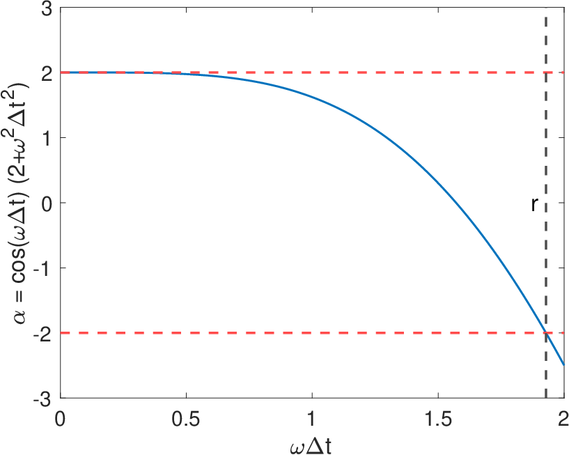
From Figure 9 we see that for where . This choice of the time-step corresponds to a requirement of at least four time-steps per iteration. However, the WaveHoltz kernel evaluates to a constant if four time-steps are taken for the forward solve. Thus at least five time-steps are needed for stability.
Appendix B Accuracy of the Discrete Filter Transfer Function
Consider the (continous) rescaled filter transfer function,
with discrete analogue (via trapezoidal rule)
Let us now take a look at the rescaled discrete filter function, . It is sufficient to consider only the range , which we plot in Figure 10.


From Figure 10 we see that it is possible to integrate and get eigenvalues of the WHI operator to be larger than one for a small range near resonance, . To get a sense of the size of this gap, we perform a simple bisection where we find the leftmost point such that for increasing number of quadrature points . We plot the result below in Figure 11.

From Figure 11 we see that, perhaps unsurprisingly, the gap shrinks with increasing number of quadrature points. The curve in red in Figure 11 indicates the bound
so that we see that this gap shrinks as . Moreover, if then . For , we may thus obtain convergence of the iteration if it can be guaranteed the time-step is chosen such that .
References
- [1] T. Airaksinen, A. Pennanen, and J. Toivanen, A damping preconditioner for time-harmonic wave equations in fluid and elastic material, Journal of computational physics, 228 (2009), pp. 1466–1479.
- [2] R. Anderson, J. Andrej, A. Barker, J. Bramwell, J.-S. Camier, J. Cerveny, V. Dobrev, Y. Dudouit, A. Fisher, T. Kolev, W. Pazner, M. Stowell, V. Tomov, I. Akkerman, J. Dahm, D. Medina, and S. Zampini, MFEM: A modular finite element methods library, Computers & Mathematics with Applications, 81 (2021), pp. 42–74.
- [3] D. Appelö, F. Garcia, and O. Runborg, WaveHoltz: Iterative solution of the Helmholtz equation via the wave equation, SIAM Journal on Scientific Computing, 42 (2020), pp. A1950–A1983.
- [4] D. Appelö and T. Hagstrom, An energy-based discontinuous Galerkin discretization of the elastic wave equation in second order form, Comput. Meth. Appl. Mech. Engrg., 338 (2018), pp. 362–391.
- [5] D. Appelö and G. Kreiss, A new absorbing layer for elastic waves, Journal of Computational Physics, 215 (2006), pp. 642–660.
- [6] D. Appelö and N. A. Petersson, A stable finite difference method for the elastic wave equation on complex geometries with free surfaces, Communications in Computational Physics, 5 (2009), pp. 84–107.
- [7] I. Babuška and S. Sauter, Is the pollution effect of the FEM avoidable for the Helmholtz equation considering high wave numbers?, SIAM Journal on Numerical Analysis, 34 (1997), pp. 2392–2423.
- [8] A. H. Baker, T. V. Kolev, and U. M. Yang, Improving algebraic multigrid interpolation operators for linear elasticity problems, Numerical Linear Algebra with Applications, 17 (2010), pp. 495–517.
- [9] M. M. Baumann, Fast Iterative Solution of the Time-Harmonic Elastic Wave Equation at Multiple Frequencies, PhD thesis, PhD thesis, Delft University of Technology, 2018.
- [10] E. Bécache, S. Fauqueux, and P. Joly, Stability of perfectly matched layers, group velocities and anisotropic waves, J. Comput. Phys., 188 (2003), pp. 399–433.
- [11] M. Belonosov, V. Kostin, D. Neklyudov, and V. Tcheverda, 3D numerical simulation of elastic waves with a frequency-domain iterative solver, Geophysics, 83 (2018), pp. T333–T344.
- [12] M. Bristeau, R. Glowinski, and J. Périaux, Controllability methods for the computation of time-periodic solutions; application to scattering, Journal of Computational Physics, 147 (1998), pp. 265–292.
- [13] R. Brunet, V. Dolean, and M. J. Gander, Can classical Schwarz methods for time-harmonic elastic waves converge?, in Domain Decomposition Methods in Science and Engineering XXV, Cham, 2020, Springer International Publishing, pp. 425–432.
- [14] R. Brunet, V. Dolean, and M. J. Gander, Natural domain decomposition algorithms for the solution of time-harmonic elastic waves, SIAM Journal on Scientific Computing, 42 (2020), pp. A3313–A3339.
- [15] T. Chaumont-Frelet, M. J. Grote, S. Lanteri, and J. H. Tang, A controllability method for Maxwell’s equations, 2021.
- [16] J. D. De Basabe, M. K. Sen, and M. F. Wheeler, The interior penalty discontinuous Galerkin method for elastic wave propagation: grid dispersion, Geophysical Journal International, 175 (2008), pp. 83–93.
- [17] A. El Kacimi and O. Laghrouche, Wavelet based ILU preconditioners for the numerical solution by PUFEM of high frequency elastic wave scattering, Journal of Computational Physics, 230 (2011), pp. 3119–3134.
- [18] B. Engquist and L. Ying, Sweeping preconditioner for the Helmholtz equation: hierarchical matrix representation, Communications on pure and applied mathematics, 64 (2011), pp. 697–735.
- [19] , Sweeping preconditioner for the Helmholtz equation: moving perfectly matched layers, Multiscale Modeling & Simulation, 9 (2011), pp. 686–710.
- [20] Y. Erlangga, Advances in iterative methods and preconditioners for the Helmholtz equation, Archives of Computational Methods in Engineering, 15 (2008), pp. 37–66.
- [21] O. Ernst and M. Gander, Why it is difficult to solve Helmholtz problems with classical iterative methods, in Numerical analysis of multiscale problems, Springer, 2012, pp. 325–363.
- [22] M. Gander and H. Zhang, A class of iterative solvers for the Helmholtz equation: Factorizations, sweeping preconditioners, source transfer, single layer potentials, polarized traces, and optimized Schwarz methods, SIAM Review, 61 (2019), pp. 3–76.
- [23] F. Garcia, D. Appelö, and O. Runborg, Extensions and analysis of an iterative solution of the Helmholtz equation via the wave equation, in preparation.
- [24] D. Gordon and R. Gordon, Robust and highly scalable parallel solution of the Helmholtz equation with large wave numbers, Journal of Computational and Applied Mathematics, 237 (2013), pp. 182–196.
- [25] M. Grote and J. Tang, On controllability methods for the Helmholtz equation, Journal of Computational and Applied Mathematics, 358 (2019), pp. 306–326.
- [26] M. J. Grote, A. Schneebeli, and D. Schötzau, Discontinuous Galerkin finite element method for the wave equation, SIAM Journal on Numerical Analysis, 44 (2006), pp. 2408–2431.
- [27] J. Hoe Tang, R. Brossier, and L. Métivier, Solving frequency-domain elastic wave equations via parallel controllability methods, in First International Meeting for Applied Geoscience & Energy, Society of Exploration Geophysicists, 2021, pp. 2470–2474.
- [28] H.-O. Kreiss and J. Oliger, Comparison of accurate methods for the integration of hyperbolic equations, Tellus, 24 (1972), pp. 199–215.
- [29] R. J. LeVeque, Finite volume methods for hyperbolic problems, Cambridge University Press, Cambridge, 2002.
- [30] Y. Li, L. Métivier, R. Brossier, B. Han, and J. Virieux, 2d and 3d frequency-domain elastic wave modeling in complex media with a parallel iterative solver, Geophysics, 80 (2015), pp. T101–T118.
- [31] Marcus J. Grote, Frédéric Nataf, Jet Hoe Tang, and Pierre-Henri Tournier, Parallel controllability methods for the Helmholtz equation, Computer Methods in Applied Mechanics and Engineering, 362 (2020), p. 112846.
- [32] S. Mönkölä, E. Heikkola, A. Pennanen, and T. Rossi, Time-harmonic elasticity with controllability and higher-order discretization methods, Journal of Computational Physics, 227 (2008), pp. 5513–5534.
- [33] Z. Peng and D. Appelö, EM-Waveholtz: A flexible frequency-domain method built from time-domain solvers, arXiv preprint arXiv:2103.14789, (2021).
- [34] G. Rizzuti and W. Mulder, Multigrid-based ‘shifted-Laplacian’ preconditioning for the time-harmonic elastic wave equation, Journal of Computational Physics, 317 (2016), pp. 47–65.
- [35] K. Shahbazi, An explicit expression for the penalty parameter of the interior penalty method, Journal of Computational Physics, 205 (2005), pp. 401–407.
- [36] C. C. Stolk, A time-domain preconditioner for the Helmholtz equation, 2020.
- [37] E. Treister, Shifted Laplacian multigrid for the elastic Helmholtz equation, 2018.
- [38] P. Tsuji, J. Poulson, B. Engquist, and L. Ying, Sweeping preconditioners for elastic wave propagation with spectral element methods, ESAIM: Mathematical Modelling and Numerical Analysis-Modélisation Mathématique et Analyse Numérique, 48 (2014), pp. 433–447.
- [39] S. Wang, M. V. de Hoop, J. Xia, and X. S. Li, Massively parallel structured multifrontal solver for time-harmonic elastic waves in 3-D anisotropic media, Geophysical Journal International, 191 (2012), pp. 346–366.