A Two-Stage Mechanism for Demand Response Markets

Consider a power system consisting of (i) an ISO, (ii) a generator that should be scheduled in the day-ahead market, (iii) a fast-acting reserve from which the ISO can purchase energy in the spot market to balance real-time demand-supply mismatches, (iv) a renewable energy source such as solar or wind, (v) $n$ demand response-providing loads which we refer to henceforth as the DR loads, and (vi) inelastic loads.

We divide time into days and each day into several time intervals. There are often constraints such as ramp rates that couple energy generation across different time intervals of a day, and constraints such as total energy requirements (eg., charge requirements of electric vehicles) that couple the demand across different time intervals of a day. However, for ease of exposition of the main ideas, we assume that there are no inter-temporal constraints that couple generation or demand across time so that it suffices to describe the problem and the mechanism for an arbitrarily fixed time interval $t$. Hence, in all forthcoming notation, we only include the index $l\in\mathbb{N}$ denoting the day and suppress the index $t$ which denotes the time interval within the day.

Denote by $z(l)$ the net demand of inelastic loads on day $l\in\mathbb{N}$ (at the arbitrarily fixed time $t$), by which we mean the difference between the sum demand of all inelastic loads and the renewable energy that is produced on day $l$ (at the arbitrarily fixed time $t$). A quintessential feature of renewable energy sources is that the energy that they produce on any day $l$ is a random variable in the day-ahead market. Consequently, $z(l)$ is a random variable in the day-ahead market and we denote by $\theta_{z}$ its probability distribution. We also assume that $\{z(1),z(2),\ldots,\}$ is an Independent and Identically Distributed (IID) sequence.

Denote by $d_{i}(l)$ the baseline demand of DR load $i$ on day $l$, $i\in\{1,\ldots,n\}$ and $l\in\mathbb{N}.$ By baseline demand $d_{i}(l)$, we mean the energy that DR load $i$ consumes on day $l$ if it does not adjust its energy consumption for demand response. To keep the analysis simple, we quantize power so that $d_{i}(l)\in\{0,1,\ldots,d_{\mathrm{max}}\}$ for all $i,l.$

Real-world loads exhibit two important characteristics: (i) Their baselines could be different on different days, and (ii) their appetite for reducing energy consumption could be different on different days. We model these two factors by the notion of a type. Hence, the baseline of a DR load and its appetite for reducing energy consumption being different on different days is tantamount to its type being different on different days. Section III-D provides a precise operational meaning for the type of a DR load. We denote by $\Delta$ the type space of the DR loads.

We model the time variation of a DR load $i$’s type by modeling it as a random variable that is drawn independently on each day $l$ from a probability distribution $\theta_{i}.$ Hence, denoting by $\delta_{i}(l)\in\Delta$ the type of DR load $i$ on day $l$, the sequence $\{\boldsymbol{\delta}(1),\boldsymbol{\delta}(2),\ldots\}$ is an IID sequence of random variables with $\boldsymbol{\delta}(1)\sim\theta_{1}\times\ldots\times\theta_{n}=\mathrel{\mathop{\mathchar 58\relax}}\theta_{\otimes}.$

Both the type distribution $\theta_{i}$ and the type realization $\{\delta_{i}(1),\delta_{i}(2),\ldots\}$ of DR load $i$ are private knowledge of the load. Moreover, these quantities are revealed to the load at different times. Specifically, in the day-ahead market, the load does not know precisely its baseline the next day, nor does it know precisely its appetite for reducing consumption the next day. Rather, it only knows the probability distribution $\theta_{i}$ according to which its type is drawn. The load observes its type realization $\delta_{i}(l)$ only on day $l$.

Note that we have assumed the type distribution of each DR load to remain the same on all days. This is only for ease of exposition and to simplify to some extent the already complicated notation. With minor modifications, the results of this paper will continue to hold even in the case when the type distributions are different on different days but the number of different distributions in $L$ days is $o(L).$

Providing demand response involves the DR loads reducing their energy consumption from their baseline to a lower quantity during times of power supply shortage. Power supply shortages could occur, for example, due to low renewable energy generation. Power consumption reductions come at a certain discomfort or productivity loss to the DR loads which we capture by means of a cost function. The cost incurred by a DR load on any given day is a function of both the consumption reduction and its type on that particular day. Specifically, we denote by $c_{i}(x,\delta_{i}(l))\in\mathbb{R}$ the cost incurred by DR load $i$ on day $l$ for consuming $x$ units of energy below its baseline (recall that the type $\delta_{i}(l)$ specifies the DR load’s baseline on day $l$).

Generators that have low ramp rates must have their power dispatch scheduled well in advance of the time of power delivery, and this is typically done in the day-ahead market. We denote by $c_{g}\mathrel{\mathop{\mathchar 58\relax}}\mathbb{R}_{+}\to\mathbb{R}$ the production function of the generator so that $c_{g}(x)$ specifies the cost that the generator incurs for producing $x$ units of energy.

We assume the availability of a fast-acting reserve generator that can produce or consume energy in real time to balance real-time demand-supply mismatches. We denote by $c_{r}\mathrel{\mathop{\mathchar 58\relax}}\mathbb{R}\to\mathbb{R}$ the production function of the reserve so that $c_{r}(x)$ specifies the cost incurred by the reserve generator for producing $x$ units of energy.

On any day $l$, the ISO observes the supply shortage $z(l)$ and each DR load $i$ observes its type ${\delta}_{i}(l)$. The type realizations are private to the DR loads but the ISO requires their knowledge to determine the optimal consumption reduction of each DR load on day $l$. Hence, the ISO requests the DR loads to report their types, but for strategic reasons that will become clear in Section III-J, they may not bid their types truthfully. Hence, we denote by $\widehat{\delta}_{i}(l)$ the type reported by DR load $i$ on day $l.$ A demand response policy $\boldsymbol{\pi}\mathrel{\mathop{\mathchar 58\relax}}\mathbb{R}\times\Delta^{n}\to\mathbb{R}^{n}$ is a rule by which the ISO determines the amount by which each DR load should reduce its energy consumption from its baseline as a function of $z(l)$ and the reported types ${\widehat{\boldsymbol{\delta}}}(l)$.

There are two decisions that the ISO should compute in the day-ahead market:

1. (i)

   the power dispatch of the generator, and

2. (ii)

   the demand response policy of the DR loads.

These quantities must be computed only based on the information that is available in the day-ahead market, namely, the type distributions $\theta_{1},\ldots,\theta_{n}$ of the DR loads, which are known privately to them, and the distribution $\theta_{z}$ of the net demand of the inelastic loads, which is public knowledge.

Since the type distributions are private to the DR loads, the ISO requests the DR loads to report them in the day-ahead market. However, for strategic reasons that we describe in Section III-J, the DR loads may not bid their type distributions truthfully and so we denote by $\widehat{\theta}_{i}$ the type distribution reported by DR load $i.$

Suppose for a moment that the DR loads bid their type distributions truthfully so that $\widehat{\theta}_{\otimes}\coloneqq\widehat{\theta}_{1}\times\ldots\times\widehat{\theta}_{n}=\theta_{\otimes}$, and that they bid their type realizations truthfully in real time so that $\boldsymbol{\widehat{\delta}}(l)=\boldsymbol{\delta}(l)$ for all $l$. How should the ISO compute the power dispatch of the generator and the demand response policy of the DR loads in this case?

To answer this, suppose that energy dispatch of the generator is chosen to be $g$ and that the demand response policy is chosen to be $\boldsymbol{\pi}$. Then, the demand-supply mismatch that occurs in real time on any day $l$ is

where $\pi_{i}(z(l),\widehat{\boldsymbol{\delta}}(l))$ denotes the $i$th component of $\boldsymbol{\pi}(z(l),\widehat{\boldsymbol{\delta}}(l))$ and $\widehat{d}_{i}(l)$ denotes the baseline reported by DR load $i$ on day $l$ (which, recall, is specified by $\widehat{\delta}_{i}(l)$). The ISO must purchase $g_{r}(l)$ units of energy from the reserve at cost $c_{r}(g_{r}(l))$. Note that $g_{r}(l)$ is a random variable in the day-ahead market whose distribution depends on $\theta_{\otimes},$ which we have assumed for the moment is known to the ISO. Consequently, the expected social cost — defined as the total cost incurred by the generator, the reserve, and the DR loads — on day $l$ is

The goal of the ISO in the day-ahead market is to minimize the total expected social cost the following day and therefore determines the power dispatch $g^{*}_{\widehat{\theta}_{\otimes}}$ and demand response policy $\boldsymbol{\pi}^{*}_{\widehat{\theta}_{\otimes}}$ as

We denote by $W^{*}(\widehat{\theta}_{\otimes})$ the optimal value of the above objective.

The problem of course is that the reported type distributions $(\widehat{\theta}_{1},\ldots,\widehat{\theta}_{n})$ may not be equal to the true type distributions $(\theta_{1},\ldots,\theta_{n})$, and so the decision $(g^{*}_{\widehat{\theta}_{\otimes}},\pi^{*}_{\widehat{\theta}_{\otimes}})$ which the ISO computes in the day-ahead market may not be equal to the optimal decision $(g^{*}_{\theta_{\otimes}},\pi^{*}_{\theta_{\otimes}})$. We describe in Section IV the mechanism by which the ISO can elicit the type distributions truthfully.

It is worth noting that the optimal power dispatch and demand response policy are functions of only $\theta_{\otimes}$ and $\theta_{z}$ which we assume remain the same on all days. Hence, it suffices for the DR loads to report their type distributions just once and for the ISO to compute the optimal power dispatch and demand response policy just once, namely, in the day-ahead market before day $1$. It can reuse these decisions on all days without any loss of optimality. As mentioned before, with minor modifications, the results of this paper extend to a more general case wherein the distributions are different on different days but the number of different distributions in $L$ days is $o(L).$

After the day-ahead decisions are made, the net demand $z(l)$ of the inelastic loads and the type profile $\boldsymbol{\delta}(l)$ of the DR loads realize on day $l$. The ISO requests the DR loads to report their type realizations and we denote by $\widehat{\delta}_{i}(l)$ the type reported by DR load $i$ on day $l,$ which may or may not be equal to its true type $\delta_{i}(l).$ The ISO then computes $\boldsymbol{\pi}^{*}_{\widehat{\theta}_{\otimes}}(z(l),\boldsymbol{\widehat{\delta}}(l))$, informs each DR load the amount by which it should reduce its consumption, and purchases the residual mismatch from the spot market. Each DR load $i$ is contractually obligated to set its actual energy consumption $y_{i}(l)$ as

where $\pi^{*}_{\widehat{\theta}_{\otimes},i}(z(l),\widehat{\boldsymbol{\delta}}(l))$ denotes the $i$th component of $\boldsymbol{\pi}^{*}_{\widehat{\theta}_{\otimes}}(z(l),\boldsymbol{\widehat{\delta}}(l)).$ Note that the ISO can check for each DR load $i$ whether its actual energy consumption satisfies the above equality, and declare it to be non-compliant with the DR program if not.

Note also that the ISO conducting the above check does not imply that a DR load $i$ truthfully reduces its energy consumption by $\pi_{\widehat{\theta}_{\otimes},i}^{*}(z(l),\boldsymbol{\widehat{\delta}}(l))$ since it could misreport its baseline. For example, it could inflate its baseline by reporting $\widehat{d}_{i}(l)>d_{i}(l)$ to give the impression of curtailing consumption without actually doing so. The mechanism presented in Section IV incentivizes the DR loads to truthfully report their baselines, thereby obligating them to reduce their real-time consumption by the ISO-specified amounts.

As described in Section III-F, the DR loads only know their type distributions in the day-ahead market which they have to report to the ISO. We denote by $\sigma_{i}\mathrel{\mathop{\mathchar 58\relax}}\Theta\to\Theta$ the day-ahead bidding strategy of DR load $i$ so that $\widehat{\theta}_{i}=\sigma_{i}(\theta_{i})$. Here, $\Theta$ denotes the set of probability distributions on $\Delta$.

In real time, DR loads bid their type realizations. We allow for the type bid $\widehat{\delta}_{i}(l)$ of DR load $i$ to be constructed based on all information that is available to it until day $l$, and in accordance with any arbitrary, randomized, history-dependent policy. Hence, a real-time bidding policy $\phi$ of DR load $i$ specifies $\mathbb{P}_{\phi}(\widehat{\delta}_{i}(l)|\delta_{i}^{l},{(\pi^{*}_{\widehat{\theta}_{\otimes},i})}^{l-1},g^{*}_{\widehat{\theta}_{\otimes}})$ for each $l\in\mathbb{N}$. I.e., it specifies a probability distribution over the type space $\Delta$ according to which $\widehat{\delta}_{i}(l)$ is chosen as a function of all observations available to DR load $i$ until day $l$. We denote by $\Phi_{i}$ the set of all real-time bidding policies.

Observe that the real-time bidding policy is a rule which specifies how a DR load should construct its type bid on any given day. While the output of the rule on any given day is a random variable which depends on the realization of the type sequence $\boldsymbol{\delta}^{\infty},$ there is nothing random about the rule itself. A load without any loss of generality can choose the rule in the day-ahead market corresponding to day $1$, and as a function of $\theta_{i}$ — the only information that is available to it at that time. This observation leads to the notion of a real-time bidding strategy. A real-time bidding strategy of DR load $i$ is a function that maps its type distribution $\theta_{i}$ to a real-time bidding policy in $\Phi_{i}.$ We denote by $\mu_{i}\mathrel{\mathop{\mathchar 58\relax}}\Theta\to\Phi_{i}$ the real-time bidding strategy of DR load $i$ so that $\mu_{i}(\theta_{i})$ is its real-time bidding policy.

Note that both the day-ahead bidding strategy $\sigma_{i}$ and the real-time bidding strategy $\mu_{i}$ are functions on the set $\Theta$, and a DR load $i$ without any loss of generality can choose these functions “offline,” i.e., even before it observes $\theta_{i}$.

We refer to the combination $S_{i}\coloneqq(\sigma_{i},\mu_{i})$ as the strategy of DR load $i$ and denote by $\mathcal{S}_{i}$ the set of strategies available to DR load $i.$ Note that once all DR loads fix their strategies, a functional relationship is established between $\boldsymbol{\widehat{\delta}}^{\infty}$ and $\boldsymbol{\delta}^{\infty},$ and all random variables become well defined.

We denote by $\mathcal{T}_{i}$ the set of truthful strategies available to DR load $i.$

The ISO has for every $(i,l)\in\{1,\ldots,n\}\times\mathbb{N}$ a payment rule $p_{i,l}\mathrel{\mathop{\mathchar 58\relax}}\theta_{\otimes}\times\Delta^{n\times l}\to\mathbb{R}$ that determines the payment that DR load $i$ receives on day $l$ for setting its consumption on that day to be equal to $\widehat{d}_{i}(l)-\pi^{*}_{\widehat{\theta}_{\otimes},i}(z(l),\boldsymbol{\widehat{\delta}}(l)).$ The payment is determined as a function of all information that is available to the ISO until day $l$, namely, $\widehat{\theta}_{\otimes}$ and $\widehat{\boldsymbol{\delta}}^{l}$.

The utility that DR load $i$ accrues on day $l$ is defined as

and its long-term average utility is defined as

Note that the above utility is a function not only of the strategy $S_{i}$ that DR load $i$ employs, but also of the strategies $\mathbf{S}_{-i}$ that the other DR loads employ. We will return to this point in the next subsection. Before that, it is necessary to recall the notion of a non-bankrupting strategy that was recently introduced in [15].

To elaborate, note that when the cost function of a DR load is bounded, the only way for its long-term average utility to be $-\infty$ is for its long-term average payment to be $-\infty,$ i.e., it pays an infinite sum to the ISO on average. Hence, the above definition essentially states that a DR load’s strategy is non-bankrupting if it is guaranteed to not expend an infinite amount by employing that strategy, regardless of what strategies the other DR loads employ and what their type distributions are.

There are three problems that the ISO faces in operating the grid optimally. The first is that the optimal day-ahead decision $(g^{*}_{\theta_{\otimes}},\boldsymbol{\pi}^{*}_{\theta_{\otimes}})$ is a function of the type distributions $\theta_{1},\ldots,\theta_{n}$ which may not be reported truthfully. Secondly, even if the ISO were to somehow compute the optimal day-ahead decisions, the optimal real-time curtailment $\boldsymbol{\pi}^{*}_{{\theta}_{\otimes}}(z(l),\boldsymbol{\delta}(l))$ on any day $l$ is a function of the type realizations $\delta_{1}(l),\ldots,\delta_{n}(l)$ which may not be reported truthfully. Finally, the ISO cannot verify if a DR load $i$ faithfully reduces its consumption by $\pi_{\widehat{\theta}_{\otimes},i}^{*}(z(l),\widehat{\boldsymbol{\delta}}(l))$ since it can only observe its actual consumption $y_{i}(l)$ and not its counterfactual baseline $d_{i}(l).$

All of these problems disappear if each DR load $i$ employs a truthful strategy. However, note from (3) that the utility of a DR load $i$ is a function not only of the strategy $S_{i}$ that it employs, but also of the strategies $\mathbf{S}_{-i}$ that the other DR loads employ. Consequently, a DR load $i$ may not employ a truthful strategy if there exists $(\mathbf{S}_{-i},\theta_{\otimes})$ such that with some non-zero probability, DR load $i$ accrues a larger long-term average utility by employing a non-truthful strategy. This brings us to the mechanism design problem. We wish to design the payment rule $\{p_{i,l}\mathrel{\mathop{\mathchar 58\relax}}(i,l)\in\{1,\ldots,n\}\times\mathbb{N}\}$ such that each DR load $i$’s utility (3) is almost surely maximized by choosing $S_{i}\in\mathcal{T}_{i}$ regardless of what non-bankrupting strategy profile $\boldsymbol{S}_{-i}$ the other DR loads employ, and regardless of what ${\theta}_{\otimes}$ is. The next section presents such a payment rule.

For every DR load $i,$ $i\in\{1,\ldots,n\},$ the first stage payment that it receives on any day $l$ is the Vickrey-Clarke-Groves (VCG) payment defined as

where $W^{*}(\widehat{\theta}_{\otimes,-i})$ denotes the optimal social cost that would be attained if DR load $i$ were absent.

One of the primary functions of the second-stage settlement is to penalize DR loads for type bids whose empirical distributions are not consistent with the type distribution that they bid in the day-ahead market. Towards this, define for each $i\in\{1,\ldots,n\},$ $\nu\in\Delta$ and $L\in\mathbb{N}$, the empirical deviation

where $\widehat{\theta}_{i}(\nu)$ denotes the probability that a random variable distributed according to $\widehat{\theta}_{i}$ takes the value $\nu$. It is easy to see that if DR load $i$ employs a truthful strategy, then $f_{i,\nu}(L)\to 0$ almost surely for all $\nu\in\Delta$.

Similarly, for every $i\in\{1,\ldots,n\},$ $\nu\in\Delta,$ $\boldsymbol{\eta}\in\Delta^{n-1},$ and $L\in\mathbb{N},$ define

and note that $h_{i,\nu,\boldsymbol{\eta}}(L)\to 0$ almost surely if the DR loads employ a truthful strategy.

The second stage settlement rule checks on each day $L$ if $f_{i,\nu}(L)$ or $h_{i,\nu,\boldsymbol{\eta}}(L)$ exceeds a certain threshold $r(L)$ for some $(\nu,\boldsymbol{\eta})$ and imposes penalty $J_{p}(L)$ if one of them does. Towards this, define

How should the threshold sequence $\{r\}$ and the penalty sequence $\{J_{p}\}$ be chosen? The sequence $\{r\}$ should be chosen to balance two competing objectives. On the one hand, $r(l)$ must tend to $0$ as $l\to\infty$ since otherwise, the set of type bids that fall within the threshold will be “large,” thereby violating incentive compatibility. However, if the sequence shrinks to $0$ too quickly, then even truthful type bids may fall outside the threshold often, thereby incurring penalties often which in turn violates individual rationality. To balance the objectives, $\{r\}$ must be chosen such that

and for some $\gamma>0,$

The penalty sequence must be chosen to satisfy

See [15, Section III] for further intuition for these conditions.

The second stage settlement that DR load $i$, $i\in\{1,\ldots,n\},$ receives on any day $l$, $l\in\mathbb{N},$ is defined as

The total payment received by DR load $i$ on day $l$ is the sum of the first-stage payment and the second-stage settlement. I.e.,

We now state the main result of the paper.

The posted price mechanism involves the ISO announcing a rebate for consumption reductions during times of power supply shortage. The DR loads react to the announced price and optimize their energy consumption which leads to energy consumption reductions.

To elaborate, denote by $p$ the rebate that the ISO provides a DR load for every unit of reduction in its energy consumption. On each day $l,$ each DR load $i$ determines its consumption reduction $x^{*}_{i}(l)$ as

Consequently, the total demand-supply mismatch on day $l$ is

which the ISO must purchase from the spot market on day $l.$ This costs $c_{r}(g_{r}(l))$ on day $l.$ Consequently, the social cost incurred on day $l$ equals

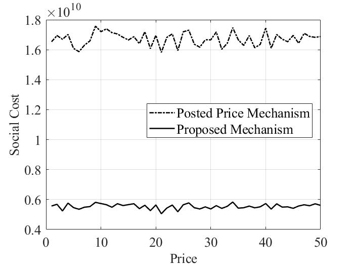
Note that the above quantity is a function of the price $p$ offered by the ISO, and in Fig. 2, the dotted curve plots the average social cost incurred by the posted price mechanism as a function of the price $p,$ averaged over $1000$ days. Section V-C contains further details.

The mechanism proposed in the Section IV incentivizes each DR load to bid its type distribution and type realizations truthfully, thereby allowing the system operator to determine the optimal energy consumption reductions and reserve generation on each day $l$ as a solution to optimization program

The optimal value of this program is a random variable that depends on the realization of $\boldsymbol{\delta}(l).$ The solid curve of Fig. 2 plots the optimal value averaged over a duration of $1000$ days. Note that the above quantity is independent of the price $p$ defined as a part of the posted price mechanism. The variation of the solid curve across different values of $p$ stems solely from averaging a random variable over a finite number of realizations.

For simulations, we assume a system with $10000$ demand response-providing loads, i.e., $n=10000$. We take all costs to be quadratic so that $c_{i}(x,\delta_{i}(l))=\frac{\delta_{i}(l)}{2}x^{2}$ for all $i,l$ and $c_{r}(x)=5x^{2}$. The distribution of $\delta_{i}(l)$ is taken to be uniform in $\{1,\ldots,10\}$ for all $i,l$, and the net demand of the inelastic loads $z(l)$ on each day $l$ is taken to be uniformly distributed in the interval [$0$J, $100$J]. We simulate both the posted price mechanism and the proposed mechanism for a duration of $1000$ days.

An alert reader would have noticed that in the description of the posted price mechanism, we have implicitly assumed the ISO to know the baseline of each DR load — an advantage not assumed for the ISO in the proposed mechanism. In spite of this advantage, the social cost incurred by the posted price mechanism is almost thrice as large as the social cost incurred by the proposed mechanism.

References

- [1] A. R. Jordehi, “Optimisation of demand response in electric power systems, a review,” Renewable and sustainable energy reviews, vol. 103, pp. 308–319, 2019.
- [2] R. Deng, Z. Yang, M.-Y. Chow, and J. Chen, “A survey on demand response in smart grids: Mathematical models and approaches,” IEEE Transactions on Industrial Informatics, vol. 11, no. 3, pp. 570–582, 2015.
- [3] J. S. Vardakas, N. Zorba, and C. V. Verikoukis, “A Survey on Demand Response Programs in Smart Grids: Pricing Methods and Optimization Algorithms,” IEEE Communications Surveys & Tutorials, vol. 17, no. 1, pp. 152–178, 2015.
- [4] P. Siano, “Demand response and smart grids: A survey,” Renewable and sustainable energy reviews, vol. 30, pp. 461–478, 2014.
- [5] N. O’Connell, P. Pinson, H. Madsen, and M. O’Malley, “Benefits and challenges of electrical demand response: A critical review,” Renewable and Sustainable Energy Reviews, vol. 39, pp. 686–699, 2014.
- [6] M. Lee, O. Aslam, B. Foster, D. Kathan, J. Kwok, L. Medearis, R. Palmer, P. Sporborg, and M. Tita, “Assessment of demand response and advanced metering,” Federal Energy Regulatory Commission, Tech. Rep, 2013.
- [7] S. Kwon, L. Ntaimo, and N. Gautam, “Optimal day-ahead power procurement with renewable energy and demand response,” IEEE Transactions on Power Systems, vol. 32, no. 5, pp. 3924–3933, Sep. 2017.
- [8] S. Wang, S. Bi, and Y. A. Zhang, “Demand response management for profit maximizing energy loads in real-time electricity market,” IEEE Transactions on Power Systems, vol. 33, no. 6, pp. 6387–6396, Nov 2018.
- [9] H. Xu, A. D. Domínguez-García, and P. W. Sauer, “Data-driven coordination of distributed energy resources for active power provision,” IEEE Transactions on Power Systems, vol. 34, no. 4, pp. 3047–3058, July 2019.
- [10] W. Hogan, “Demand response pricing in organized wholesale markets,” ISO/RTO Council Comments on Demand Response Compensation in Organized Wholesale Energy Markets, vol. 13, 2010.
- [11] M. Surampudy, B. Chew, M. Keller, and T. Gibson, “2019 utility demand response market snapshot,” Smart Electric Power Alliance (SEPA), Navigant Consulting, and Peak Load Management Alliance (PLMA, Tech. Rep., 2019.
- [12] D. Muthirayan, D. Kalathil, K. Poolla, and P. Varaiya, “Baseline estimation and scheduling for demand response,” in 2018 IEEE Conference on Decision and Control (CDC), 2018, pp. 4857–4862.
- [13] ——, “Mechanism design for demand response programs,” IEEE Transactions on Smart Grid, vol. 11, no. 1, pp. 61–73, 2020.
- [14] I. Schneider, M. Roozbehani, and M. Dahleh, “An online learning framework for targeting demand response customers,” IEEE Transactions on Smart Grid, vol. 13, no. 1, pp. 293–301, 2021.
- [15] B. Satchidanandan and M. A. Dahleh, “Incentive compatibility in two-stage repeated stochastic games,” arXiv preprint arXiv:2203.10206 [econ.TH], March 2022.
- [16] S. Park, S. Ryu, Y. Choi, J. Kim, and H. Kim, “Data-driven baseline estimation of residential buildings for demand response,” Energies, vol. 8, no. 9, pp. 10 239–10 259, 2015.
- [17] J. L. Mathieu, D. S. Callaway, and S. Kiliccote, “Examining uncertainty in demand response baseline models and variability in automated responses to dynamic pricing,” in 2011 50th IEEE Conference on Decision and Control and European Control Conference, 2011, pp. 4332–4339.
- [18] X. Wang and W. Tang, “To overconsume or underconsume: Baseline manipulation in demand response programs,” in 2018 North American Power Symposium (NAPS). IEEE, 2018, pp. 1–6.
- [19] D. T. Nguyen, M. Negnevitsky, and M. de Groot, “Market-based demand response scheduling in a deregulated environment,” IEEE Transactions on Smart Grid, vol. 4, no. 4, pp. 1948–1956, 2013.
- [20] B. Xia, K.-Y. Lee, S. Shakkottai, and D. Kalathil, “A market for retail electric provider based demand response,” in 2019 IEEE 58th Conference on Decision and Control (CDC), 2019, pp. 8429–8434.
- [21] D. Muthirayan, D. Kalathil, K. Poolla, and P. Varaiya, “Mechanism design for self-reporting baselines in demand response,” in 2016 American Control Conference (ACC), 2016, pp. 1446–1451.
- [22] D. Muthirayan, E. Baeyens, P. Chakraborty, K. Poolla, and P. P. Khargonekar, “A minimal incentive-based demand response program with self reported baseline mechanism,” IEEE Transactions on Smart Grid, vol. 11, no. 3, pp. 2195–2207, 2020.
- [23] D. Muthirayan, D. Kalathil, S. Li, K. Poolla, and P. Varaiya, “Selling demand response using options,” IEEE Transactions on Smart Grid, vol. 12, no. 1, pp. 279–288, 2021.
- [24] Y. Chen, W. S. Lin, F. Han, Y.-H. Yang, Z. Safar, and K. J. R. Liu, “A cheat-proof game theoretic demand response scheme for smart grids,” in 2012 IEEE International Conference on Communications (ICC), 2012, pp. 3362–3366.
- [25] A. Ramos, C. De Jonghe, D. Six, and R. Belmans, “Asymmetry of information and demand response incentives in energy markets,” in 2013 10th International Conference on the European Energy Market (EEM), 2013, pp. 1–8.
- [26] D. G. Dobakhshari and V. Gupta, “A contract design approach for phantom demand response,” IEEE Transactions on Automatic Control, vol. 64, no. 5, pp. 1974–1988, 2019.
List of Symbols