Gamma/Hadron Separation with the HAWC ObservatoryJournal: Nuclear Instruments and Methods in Physics Research Section A
Abstract
The High Altitude Water Cherenkov (HAWC) gamma-ray observatory observes atmospheric showers produced by incident gamma rays and cosmic rays with energy from 300 GeV to more than 100 TeV. A crucial phase in analyzing gamma-ray sources using ground-based gamma-ray detectors like HAWC is to identify the showers produced by gamma rays or hadrons. The HAWC observatory records roughly 25,000 events per second, with hadrons representing the vast majority () of these events. The standard gamma/hadron separation technique in HAWC uses a simple rectangular cut involving only two parameters. This work describes the implementation of more sophisticated gamma/hadron separation techniques, via machine learning methods (boosted decision trees and neural networks), and summarizes the resulting improvements in gamma/hadron separation obtained in HAWC.
Keywords:
High Energy , Crab Nebula , G/H separation , Machine Learning1 Introduction
Technological advances have enabled the expansion of the study of the cosmos to wavebands outside the small window in the optical region. The most energetic astrophysical sources emit radiation primarily in the gamma-ray band. One of the crucial issues in using ground-based detectors to study gamma-ray sources at Very High Energy (50 GeV - 100 TeV) and Ultra-High Energy (100 TeV - 100 PeV) is that the vast majority () of air showers detected come from cosmic rays, rather than gamma rays.
Ground-based gamma-ray observatories detect the passage of secondary particles produced after a primary particle impinges on an atmospheric nucleus, leading to the generation of an Extensive Air Shower (EAS). Using ground level data, EAS properties can be characterized via a set of parameters, and then used to deduce the nature of the primary particle. While gamma-ray induced showers contain mainly positrons, electrons, and gamma rays11 1 Though they may contain some muons, their numbers are small., hadron-induced showers contain muons from the decay of secondary charged pions and kaons. These muons, typically created with high transverse momentum, result in hadronic showers being more spread out, with a multi-core structure, compared to gamma-ray-induced showers, which are more compact, with a single-core structure [1].
Machine Learning Techniques (MLT) are a set of statistical and computer algorithms that can be used to build complex, non-linear, models from data, to tackle a broad range of tasks, including some in gamma-ray astronomy. On the specific task of gamma/hadron separation (hereafter simply G/H separation), ground-based gamma-ray observatories like HEGRA [2], MAGIC [3], H.E.S.S. [4], VERITAS [5], ARGO-YBJ [6], and LHAASO-WCDA [7], among others, have reported excellent results using such techniques.
1.1 The HAWC Observatory
The High-Altitude Water Cherenkov (HAWC) [8] gamma-ray observatory is a second-generation ground-based instrument located on the northern slope of the Sierra Negra volcano in the state of Puebla, Mexico, at an altitude of 4,100 meters above sea level. Like its predecessor, Milagro [9, 10], HAWC is based on the water Cherenkov technique. It consists of an array of 300 water Cherenkov detectors, each made of a cylindrical metal structure, 7.3 meters in diameter and 5 meters high, containing 180,000 liters of purified water and four photomultiplier tubes (PMTs) at the bottom. The PMTs detect Cherenkov light generated by the secondary particles of the EAS as they traverse the water. The HAWC software trigger requires 28 PMT hits within a 150 ns time window, which results in roughly 25,000 events being recorded every second [11]. The direction of the primary particle is reconstructed using the PMT timing information, while the shower core is computed using the charge on the PMTs. Thus, by measuring the detected charge and time at the PMTs, HAWC can reconstruct the characteristics of the EAS [12].
Because HAWC detects 99.9% charged cosmic-ray (hadron) events, the level of background must be significantly reduced in order to perform gamma-ray observations with HAWC. The current method of G/H separation used by the HAWC collaboration applies a simple rectangular cut to the data, involving only two parameters. Cuts on these two parameters define a rectangular region containing, preferentially, gamma-ray events. Generally speaking, this is not an optimal classification strategy because the boundary between gamma-like and hadron-like events is not defined by the actual distribution of the two types of events. In addition, the performance of the two parameters depends on the size of the observed shower (they are more sensitive for large events), so determining their optimum combination is not straightforward. A non-linear classification method should, in principle, provide a more effective discriminator.
This paper describes the implementation of two new G/H separation methods in HAWC, using MLT; one based on Boosted Decision Trees (BDT) and another using Neural Networks (NN). The performance of the new techniques is compared with previously used HAWC cuts [13, 14].
The outline of the paper is as follows: Section 2 gives an overview of the key parameters generated from HAWC data, which are used as inputs in our G/H separation models. Section 3 describes the HAWC data used in our study, both Monte Carlo (MC) simulated data, as well as real data on three astrophysical sources. Section 4 describes the G/H separation models discussed in the paper, including the current (standard) methods used by HAWC, as well as our two new proposed techniques. Section 5 describes how we build the different models, including details on determining the optimal cuts for each method. Section 6 reports the performance of the various methods, comparing them via MC and real data. We conclude, in Section 7, with a discussion of the overall performance of the models, along with possible implications regarding the future improvements of our results.
2 HAWC G/H separation parameters
Among the many parameters generated by the HAWC experiment for each event, we considered those that could help to characterize the nature of the EAS, ultimately settling on seven, which we used as inputs in our G/H separation algorithms. These parameters broadly fall into three classes: those related to the energy of the event, those sensitive to the muon content of the shower, and those connected to the shower’s lateral development, via the lateral charge distribution function.
2.1 Energy parameters
Two official gamma-ray energy estimators are currently used in HAWC: one based on charge density and the second using a neural network [14]. In both estimators, the HAWC data are grouped in a 2D binning scheme consisting of a fraction hit bin, , and an energy bin, ebin. The bin is defined as fHit = nHit/nCh, where nHit is the number of PMTs activated during the event within 20 ns of the shower front, and nCh is the total number of PMTs in operation at the time. The energy bin (ebin) used in this work is given by the neural network energy estimator [14]. We use ten22 2 Note that the bin is currently not being used in standard HAWC analyses, as it has low sensitivity with the standard G/H classifiers. We nevertheless report on it here, to study the behavior of our machine learning algorithms over the full range. bins and twelve quarter-decade energy bins, starting from 316 GeV (see Table 1).
| Range (%) | ebin | |
|---|---|---|
| 0 | 4.4 – 6.7 | 2.50 |
| 1 | 6.7 – 10.5 | 2.75 |
| 2 | 10.5 – 16.2 | 3.00 |
| 3 | 16.2 – 24.7 | 3.25 |
| 4 | 24.7 – 35.6 | 3.50 |
| 5 | 35.6 – 48.5 | 3.75 |
| 6 | 48.5 – 61.8 | 4.00 |
| 7 | 61.8 – 74.0 | 4.25 |
| 8 | 74.0 – 84.0 | 4.50 |
| 9 | 84.0 – 100.0 | 4.75 |
| 5.00 | ||
| 5.25 |
2.2 Muon content parameters
Typically, the muons present in a hadronic cascade are produced at a considerable distance from both the shower axis and one another. In the HAWC detector, these lead to strong signals in widely-separated PMTs. Two HAWC parameters can be used to try to identify them:
- 1.
LIC is the log transformation of the inverse of the compactness parameter, an empirical parameter originally developed by the Milagro Collaboration [10], as described in Abeysekara et al. 2017 [13]:
LIC= = ,
where is the charge measured in the PMT with the largest effective charge far (40 m) from the shower core. When a muon passes near a PMT, the resulting charge (and, thus, LIC) will be large (see Figure 3 of Pretz et al. 2015 [15]), indicating that the shower is more likely produced by a hadron. Since gamma ray showers contain few, if any, muons, they are characterized by a small LIC value.
- 2.
disMax measures the physical distance, in meters, between the two brightest PMTs. Hadronic showers are expected to have large values of disMax, while gamma-ray showers are characterized by small values.
2.3 Lateral development parameters
In gamma-ray showers, most secondary particles are generated close to the shower axis. Thus, HAWC registers their signals near this axis, with a smooth decrease with distance from the core. Three HAWC parameters can be used to describe the lateral development of the shower:
- 1.
PINC (Parameter for IdeNtifying Cosmic rays) is a parameter that quantifies the smoothness of the lateral charge distribution function (LDF) (see Figure 4 of Abeysekara et al. 2017 [13]). Gamma-ray showers are characterized by having PMTs with a high charge near the core, and a smoothly decreasing LDF. By contrast, hadronic showers typically contain several clumps of charges caused by widely-separated muons, thus leading to a “wrinkled" LDF. PINC, in essence, is the of the difference between the effective log charge of each PMT hit () and the expected mean value () computed by averaging all PMTs within an annulus, 5 m in width, centered on the core of the air shower containing the PMT hit.
Here is the uncertainty in , based on a study of gamma shower data from the Crab [13], and is the number of annuli.
- 2.
LDFChi2 is the reduced chi-square obtained from fitting the LDF, with the expected shape given by the NKG function [16]:
,
where is the distance from the shower axis () at the observation level, in units of the Molière radius33 3 = 124 m at HAWC. (), A is the amplitude, and the shower age. Because the charge distribution is more homogeneous in a gamma-ray shower, than a hadronic one [17], the model fits better in gamma-ray events than hadronic ones.
- 3.
LDFAmp is the logarithm of the amplitude obtained from the LDF fit. Gamma-ray and hadronic events in a given fraction hit bin are expected to have different values of LDFAmp because of differences in the lateral distributions of gamma vs. hadron events.
3 Data sets
3.1 Monte Carlo Data
The Monte Carlo (MC) simulations of HAWC data are generated using a set of standard software packages (e.g., CORSIKA44 4 https://www.iap.kit.edu/corsika/, GEANT455 5 https://geant4.web.cern.ch), in combination with HAWC-specific simulations that model the PMT response. CORSIKA 7.4 [18] was used to simulate extensive air showers initiated by high energy particles in the atmosphere, using the QGSJET-II-04 and FLUKA hadronic interaction models. GEANT4 [19] was used to simulate the passage of the shower particles through the HAWC detector.
Nine species of primary particles were simulated: eight atomic nuclei66 6 H, He, C, O, Ne, Mg, Si, and Fe. (MC background), along with gamma rays (MC signal). Approximately 23 million signal and 13 million background events were generated, using a power-law energy spectrum with a spectral index of -2.0 between 5 GeV and 500 TeV, uniformly on the sky within a zenith angle below 60∘. The choice of a relatively hard spectrum results in increased statistics at higher energies at a considerable savings in computing time. For analyses which simulate the transit of a specific astrophysical source (e.g., the Crab Nebula, with a spectral index of -2.63), our simulated events must be weighted by energy and location. The number of simulated events we used was found to be sufficient for previous studies carried out by the HAWC Collaboration, such as the application of neural networks to estimate the primary particle energy in HAWC [14].
3.2 Real HAWC data on astrophysical sources
In order to test our classification models on real data, we selected all available HAWC data from June 2015 to December 2017 ( 837 live days). We explored three different sources: the Crab Nebula, and the extra-galactic sources Markarian 421 and Markarian 501.
Crab
The Crab is the remnant of the historical supernova explosion, recorded by Chinese astronomers in 1054. One of the most famous astrophysical objects77 7 Also known as M1, the first entry in the famous catalog of astronomical objects compiled by Charles Messier in the 18th century., the Crab is detected across the electromagnetic spectrum [20] and its brightness and relatively steady flux at TeV energies have made it the definitive reference/calibration source for all TeV instruments.
Markarian 421 and 501
Markarian 421 and 501 (hereafter Mrk 421 and Mrk 501) are two relatively nearby ( 150 Mpc) Active Galactic Nuclei (AGN) of the blazar variety (i.e., with jets of accelerating particles pointed towards our line of sight) [21]. They have been known to emit at very high energy ( 100 GeV) for decades, and they routinely experience outbursts during which they become even brighter than the Crab. HAWC detects them at high significance, and indeed, monitors them daily for any unusual activity [22].
3.3 Real HAWC data as background data
4 G/H separation models
The goal of the G/H separation task is to keep a majority of gamma-ray events while rejecting most hadron events. We define as the fraction of gamma-ray events passing the G/H selection, in other words, the fraction of gamma-ray events correctly classified. Conversely, we define as the fraction of hadron events passing the G/H selection cut, and thus being misclassified. Thus, our aim is to achieve a gamma efficiency () close to 1 while keeping the hadron misidentification rate () near 0.
Figure 1 shows the Receiver Operating Characteristic (ROC) curves [23] for three of the shower parameters described in Section 2. These curves, obtained from our MC simulations, illustrate the effect that varying thresholds in the different parameters have on the resulting values of and .

In the high energy bin (upper curves), the PINC and LDFChi2 parameters have a similar response, with a good (high) and an excellent (low) . Both perform significantly better than LIC at high energy. In the lower energy bin, all three parameters have roughly the same G/H performance, significantly worse than at high energy. Although PINC and LDFChi2 are highly correlated (they are both based on the LDF of the gamma shower, see B), they report different information, so we keep them both; at low energy, their performance differs more than at high energy. Lower bins typically have worse G/H performance because the shower has fewer PMTs participating in the event measurement.
In order to improve on the performance of any individual parameter, one can combine them, for example, by applying cuts on several parameters simultaneously [24]. Indeed, the current official G/H separation method in HAWC uses a simple 2 parameter cut, as described in Section 4.1.
Other more sophisticated approaches include using a likelihood ratio method to combine several parameters [17], or using MLT, as implemented successfully in the HEGRA [2] and H.E.S.S. [4] observatories, among others.
In Section 4.2, we describe the implementation, in HAWC, of two new G/H separation methods using MLT, which combine the various input parameters described in Section 2, to produce a single output value indicating the likely nature of the primary particle.
4.1 The Standard Cut (SC) in HAWC
Building on the experience with Milagro, where a cut on a single parameter was used successfully for G/H separation [10], the HAWC collaboration first implemented a similar single parameter cut, based on the compactness parameter [8] (as defined in Section 2). Subsequently, a cut on a second parameter was found to improve the performance. Rectangular cuts on these two variables as a function of the one-dimensional bins defined by , we refer to as the 1D standard cut (SC1D). Similarly, the current official, or standard cut (SC), in HAWC involves selecting only events in a rectangular region defined by the same two parameters: PINC and LIC (see Section 2), as given by the expression:
,
where and are the LIC and PINC parameter thresholds, respectively.
Events within this region are classified as gammas, while those outside are labeled as hadrons. The major difference between SC1D and the two-dimensional SC cut is that for SC, the thresholds ( and ) depend on both the fraction of PMTs activated during the event and the reconstructed primary particle energy; thus, each (, ebin) bin has a specific threshold for each parameter.
4.2 Machine Learning Techniques
In recent years, the use of computer algorithms to automatically build complex models based solely on data has been gaining ground in a range of fields, including gamma-ray astronomy. These Machine Learning Techniques (MLT) not only have the advantage of automating (and thus speeding up) repetitive tasks, but also have the potential for yielding new insights that may only be revealed as the computer processes (or “learns" from) large quantities of data.
MLT fall under two broad categories: supervised and unsupervised. The former use “labeled" data to train algorithms (e.g., classification), which can then be used to predict the labels/categories of new (unlabeled) data; the latter, by contrast, are applied to unlabeled data, allowing the algorithms themselves to uncover hidden structures in the data (e.g., via clustering) .
In this work, we apply supervised learning methods to the classification task of distinguishing between gamma rays (signal) and hadrons (background). Among the large number of machine learning algorithms, we focus on two of the most successful ones: Boosted Decision Trees (BDT) [4, 17], and Neural Networks (NN) [2, 25]. We briefly describe these two algorithms, along with their inputs in the following paragraphs.
Boosted Decision Trees (BDT)
Traditional decision trees are a simple, non-parametric flowchart-like model, that use a series of binary sequential decision nodes to split data into branches, ultimately sorting them into leaf nodes [26]. They are extensively used to tackle problems of classification (e.g., signal vs. background).
Despite their advantages, simple decision trees have a number of drawbacks, including the high variance problem, where a slight change in the data can result in a significant change in the final model; in addition, a simple binary split often leads to a lack of smoothness in the model [26]. To overcome these problems, an ensemble of trees can be combined, to ultimately produce a more powerful, boosted, model: as more trees are added, the model “learns" from the errors of the existing trees, and thus improves.
In this work, we use a Gradient boosting algorithm for our BDT model [27], as implemented in the xgboost python package88 8 https://xgboost.readthedocs.io/en/stable/. We use 500 trees, a low learning rate99 9 This learning rate affects how model weights are updated, based on the estimated error at each stage. of 0.1, to avoid large jumps around the minimum error, and a maximum tree depth of 5 nodes. For each tree, we use only a random 60% selection for each individual tree1010 10 That is, 30% of the total sample., to avoid over-fitting. The minimum value of loss reduction (error) for splitting the leaf node in each tree is set to 1. These parameters are advertised as likely to avoid overtraining. We verified this by checking that the output distributions in testing is consistent with the training output distributions.
Neural Networks (NN)
Neural Networks (NN) are non-linear algorithms that use a collection of artificial neurons to attempt to mimic a human brain [28]. Artificial neurons, like their biological counterparts, are composed of dendrites, which collect input information, a nucleus, which combines and generates a signal, and finally, an axon, that sends the information to the output. The mathematical model consists of three blocks: input parameters; a synapse function, combining the input information (i.e., a sum); and an activation function defining the output, sometimes restricting it to a specific range (e.g., sigmoid, tanh, linear). Thus, NN generally can be described as having three types of layers: an input layer, a set of hidden layers, and an output layer. The number of neurons in the input layer equals the number of input parameters. The number of hidden layers may vary, with each having any number of neurons. Typically, the neurons of the input and output layers follow a linear model (i.e., a sum as synapse function and a linear activation function, ).
Our NN models were trained using the Toolkit for MultiVariate data Analysis (TMVA), a ROOT-integrated software package that provides a user-friendly environment for processing and evaluating MLT in high-energy physics [29]. We used a multilayer Perceptron with a 7:10:10:1 architecture1111 11 Several architectures were tested, but this one provided the best performance at a reasonable computational cost.. The first layer has one neuron per input parameter. The two hidden layers have ten neurons each and a sigmoid activation function. Finally, the output layer has one neuron, giving the probability that an event is a gamma ray.
5 Building the models
Both the BDT and NN models have the potential advantage over the cuts described in Section 4.1 of combining several number of input parameters, to produce a more powerful classifier. Ultimately, however, the effectiveness of the new classifier will depend on the discriminating power of each individual parameter, as well as the correlations among them. Seven parameters were selected as inputs for our BDT and NN algorithms, as described in Section 2.
In building a model based on MLT, one commonly requires three stages: training, verification, and testing [30]. The first and second stages typically work together to build the model, while the last stage is used to evaluate the performance and stability of the model. Each stage has an independent event sample; the purpose is to avoid memorizing the events instead of learning generalizable features. We chose to split our simulation data into two equal sets: 50% for training and verification and 50% for the testing stage. Thus, the algorithms use only half of the data to build a mathematical model that can recognize the differences between gamma-ray events and charged cosmic rays, while the remaining 50% of the events are used to quantify the performance of the models. The output value for our models was defined in all cases as 1 for gamma-ray events, and 0 or -1 for hadrons, for the NN or BDT model, respectively.
Unfortunately, there is no clear answer to the question “what is the best model?”; each has its pros and cons. Both the NN and BDT show a good performance in classification; however, their training is slow. The NN response calculation is somewhat faster than the BDT (though neither significantly affects event reconstruction time). The BDT is more robust at ignoring weak variables but is more vulnerable to overtraining. Rather than training separate models in each { and ebin} bin, the data were grouped into three containers and NN and BDT models were trained on these larger groups: (low), (medium) and (high). This grouping allowed us to include more training samples per model; the use of two different (albeit correlated) energy-related input parameters (see Section 2.1), allowed our models to better interpolate over the relatively large range of bins covered by each of these containers, as suggested in [31].
Nevertheless, the cuts applied on the model output were chosen separately for each (, ebin) pair, as described in the next section.
Optimizing the cuts
Although our models are designed for the classification task, they still allow us the freedom to choose the specific cuts that will determine the separation between the signal and background classes. In this work, we set a goal of removing as much background as possible while keeping at least 50% of the signal. Section 3 describes the data set used to determine the cuts for each model. In order to define the best cut, we quantify the expected significance enhancement via the Q factor (described below). Sections 5.1 and 5.2 describe how we use this information to choose the specific cuts for the SC and MLT models, respectively; in both cases the final cuts are optimized for each individual bin.
Q factor
The quality factor, Q, of a given selection cut is a parameter commonly used in ground-based gamma-ray astronomy (e.g., Milagro [10], VERITAS [17]) to measure the expected increase in the significance of an astrophysical source, after making the cut. Thus, optimizing the Q factor predicts the best way to classify the events. We use a Gaussian approximation to the Poisson significance improvement, assuming each bin contains a sufficiently large number of events. The Q factor is thus defined as
| (1) |
5.1 Standard Cuts
The SC involves finding optimal cuts for two parameters, separately, for each bin. First, is computed using many candidate cuts on PINC and LIC, using the MC signal data. Next, is computed for these cuts using the real background set. Finally, the Q factor is calculated with Equation 1, as a function of the candidate and cuts. Figure 2 shows the results obtained for the (=3, ebin 3.0) bin, with energy between 1.00 and 1.78 TeV. The optimal cut values are those giving the maximum Q factor, with the proviso that at least 50% of the gamma-ray events are retained. This process is repeated for each (, ebin) bin. Not all bin combinations contain enough data to determine the cuts, since and the particle energy are correlated; therefore, the cuts are not computed if the sample has less than 500 events.

5.2 Machine Learning Techniques
After the training and verification stages, the BDT and NN model outputs give the probability that an event is a gamma ray: if the output value is close to 1, there is a high probability that the event is a gamma, while an output close to 0 (or -1 for BDT), means the model predicts it is likely a background event. Figure 3 shows the distribution of the NN output using the events of the =3 bin, with energy between 1.00-1.78 TeV using signal and background MC events, as well as the corresponding Q factor as a function of threshold on the NN output. The optimal cut (0.98) for the model is the one with the maximum Q factor. As in the case of the SC, the process is repeated for each {, ebin} bin to find the optimal cuts for the NN and BDT models.

6 Testing stage
The testing stage is used to evaluate and compare the models. We first test the models using samples of simulated events of known types, calculating the predicted efficiencies and Q factors (Section 6.1). Next, we applied our G/H separation models to real data, in order to obtain the actual significances of known gamma-ray sources; specifically, we looked at three well-known sources: the Crab, Markarian 421, and Markarian 501 (Section 6.2).
6.1 Testing on MC data
Our sample of signal events was taken from the MC simulation of gamma-ray showers (see Section 3.1), and is used in the training of all models (SC and MLT models).
For our background events, we chose two different samples; the first, from the set of background events in our MC simulation of hadron showers (see Section 3.1). In addition, however, we used a set of randomly selected real data events (which are known to be mostly charged cosmic rays) from a single day.
The SC model used MC signal and real data background samples for training. The MLT models were trained on MC signal and MC background events. The MC simulation agrees with real data (both signal and background) for all the discrimination variables [32]. We chose to train with MC background because we obtained slightly worse MC testing results when training with real data1212 12 We also found that the NN produced significantly worse results on real Crab signals in upper bins when trained with real data. See further discussion in A..
Having used half of our MC sample of events for the training & verification stages, we used the remaining half of our MC data sample for the testing stage. In order to compare the performance of all methods, we compute the Q factor for each {, ebin} bin for each G/H separation model, using the optimal cutoff in each case. We checked that the models were not overtrained by verifying that the model outputs on MC testing were compatible with the training outputs.
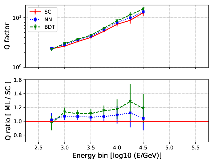
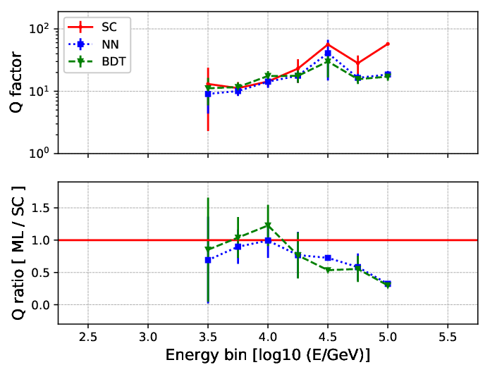
Once we have fixed the optimal cuts for each bin, we then evaluate the predicted performance on the Crab by using the testing sample, weighted appropriately to simulate transits of the Crab. Based on the MC results, the NN and BDT have better performance than the SC on the first six bins, while the SC is better for the rest of the bins. Figure 4 shows the value of the predicted Q factor of the three models for two bins (3 and 6). The bottom of the figures show the comparison of the MLT versus SC. For the =3 bin, the SC is the worst of the G/H separation models, with the NN and BDT showing an average improvement over the SC of 12% and 30%, respectively. On the other hand, for the bin, the SC reports better results than the MLT at energies above 56.2 TeV (ebin=4.75).
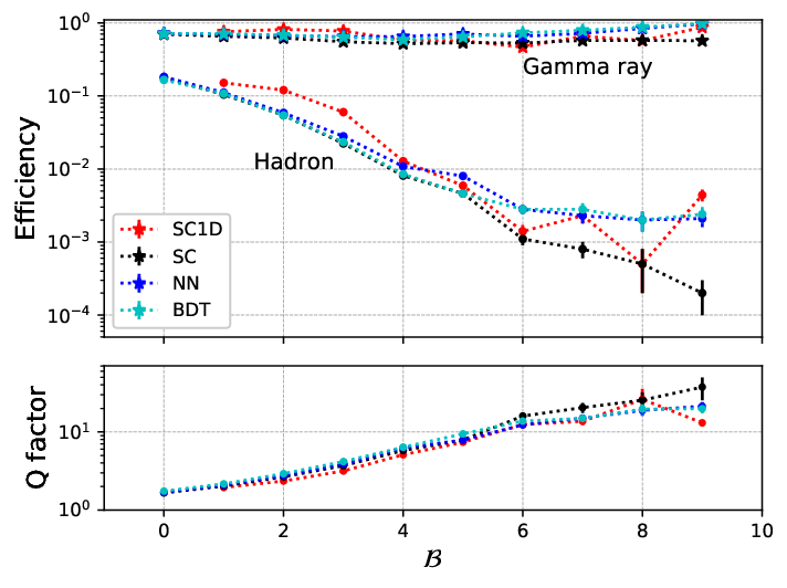
The SC1D (see Section 4.1) is the original G/H separation technique used by HAWC1313 13 Though now mostly superseded by the 2-D SC model, SC1D continues to be useful for analyses of weak or low-energy sources because it uses a less restrictive data selection than needed for applying improved energy estimators. [13]. The SC1D cuts, on PINC and compactness (and thus LiC), were optimized for each bin using a year of early Crab signal and background data. In the initial publication, G/H separation was not attempted for . Figure 5 shows and as a function of bin. The SC1D cuts were (by definition) different for each bin. For this comparison, we applied the 2D cuts separately to each {, ebin}) bin, then combined the ebins belonging to each individual bin. The MLT reports a higher at large bins. The fraction of mis-classified hadrons in the 2D models is lower in the first four bins than for SC1D, because these 2D models reject more background events. Thus, Figure 5 implies that the 2D models generally have a greater predicted Q factor, according to the MC testing comparison.
6.2 Testing on real data
In order to carry out tests on real data, we first applied our models to remove hadron events, and then proceeded to construct sky maps, using the official HAWC software in the standard way, as described in [13], with a power law spectrum of index -2.7, and a pivot energy of 7 TeV.
The G/H separation method was used to obtain the Crab significance to show the actual performance of the various methods (rather than the predicted one, based on the MC testing set), in order to compare them. In this analysis, 67 2D bins with a significance at the source position of are used1414 14 Of these, four bins belong to the =0.. For the rest of the bins (53), the maps are not included because they have too few counts or are dominated by background so that the signal is overshadowed by the noise [14]. Figure 6 shows the results for the =3 and =6 bins of the 2D G/H separation models. In the specific case of =3, the results follow the same behavior as the testing with simulation; the MLTs show an improvement over the SC. However, in the case of =6, the models have similar results except for energies greater than 56.2 TeV (ebin 4.75), where the SC is better.


In order to determine the significance as a function of the bin, we combine all ebins, thus summarizing the performance of each G/H separation model per bin. Table 2 reports the significance at the Crab location for each G/H separation method; the next three columns contain the fractional significance improvement of the 2D G/H separation models over the older SC1D; and the last two columns show the comparison between MLT and SC cuts. The last two rows report the combined significance using all 67 bins (), and the official bins only (). For most bins, the 2D models provide better results than SC1D. BDT improves the Crab significance compared to SC1D by 19% for the official bins, while the SC and NN improve, by 9% and 8%, respectively. The BDT improves over SC in every bin, while the NN improves in over half. Adding gives only a slight improvement, even with MLT methods, suggesting that this low bin requires a different approach if a useful signal is to be extracted from it.
| Significance | Difference in % between | ||||||||
| SC | NN | BDT | NN | BDT | |||||
| SC1D | SC | NN | BDT | & | & | & | & | & | |
| SC1D | SC1D | SC1D | SC | SC | |||||
| 0 | - | 15.2 | 14.7 | 16.0 | - | - | - | -3 | 5 |
| 1 | 26.9 | 27.6 | 27.5 | 28.22 | 3 | 2 | 5 | 0 | 2 |
| 2 | 37.8 | 44.1 | 44.6 | 46.4 | 17 | 18 | 23 | 1 | 5 |
| 3 | 59.2 | 62.4 | 66.1 | 72.0 | 5 | 12 | 22 | 6 | 15 |
| 4 | 70.6 | 69.7 | 76.3 | 76.2 | -1 | 8 | 8 | 10 | 9 |
| 5 | 67.3 | 71.3 | 69.7 | 80.1 | 6 | 4 | 19 | -2 | 12 |
| 6 | 52.3 | 61.5 | 48.3 | 66.0 | 18 | -8 | 26 | -21 | 7 |
| 7 | 39.1 | 47.7 | 49.2 | 50.3 | 22 | 26 | 28 | 3 | 5 |
| 8 | 27.6 | 32.8 | 35.1 | 34.8 | 19 | 27 | 26 | 7 | 6 |
| 9 | 28.2 | 28.7 | 31.3 | 31.3 | 2 | 11 | 11 | 9 | 9 |
| 1-9 | 144.0 | 155.7 | 156.9 | 170.7 | 8 | 9 | 19 | 1 | 10 |
| 0-9 | - | 156.3 | 157.5 | 171.3 | - | - | - | 1 | 10 |
We also summarize the Crab performance as a function of the energy (ebin). The flux points were obtained for the Crab in quarter-decade energy bins, using the method described in [14]. We repeated it for each G/H separation model, using a log-parabola model to fit the spectrum (see Figure 7). Table 3 reports our results, which are similar to the bin projection. The 2D models give the best G/H separation in most bins. MLT gives better results than SC at low energies, but above 41.6 TeV (ebin=4.50), the SC generally has better performance.

| ebin | Significance | |||
|---|---|---|---|---|
| SC1D | SC | NN | BDT | |
| 2.50 | 12.1 | 12.4 | 12.3 | 12.6 |
| 2.75 | 31.2 | 32.5 | 34.0 | 34.6 |
| 3.00 | 52.2 | 54.7 | 56.9 | 58.4 |
| 3.25 | 64.4 | 65.3 | 65.6 | 72.9 |
| 3.50 | 70.1 | 71.1 | 74.0 | 79.5 |
| 3.75 | 60.3 | 66.5 | 58.6 | 74.6 |
| 4.00 | 46.2 | 54.6 | 59.0 | 62.3 |
| 4.25 | 36.3 | 41.5 | 45.0 | 44.3 |
| 4.50 | 26.7 | 36.0 | 30.6 | 32.9 |
| 4.75 | 15.7 | 21.8 | 23.0 | 21.5 |
| 5.00 | 8.4 | 13.9 | 11.3 | 10.1 |
| 5.25 | 1.9 | 3.0 | 4.8 | 4.4 |
Table 4 and 5 report the significance for Mrk 421 and Mrk 501 for each bin and for the combination of all bins (0–9 and 1–9). The MLT results for Mrk 421 are consistent with those seen in the Crab in bins where both are significantly detected. MLT has similar improvement over SC for 421 as for the Crab, but all 2D methods have smaller fractional improvement over SC1D than for the Crab. However, for Mrk 501 the NN results are worse than for SC or SC1D. The performance of the SC is better than SC1D (though again not as much as for the Crab), while the BDT improvement over SC on this source is comparable to that seen for the Crab analysis. It is difficult to assess trends by bin for Mrk 501, because the source is not as strongly detected as Mrk 421 or the Crab.
| Significance | Difference in % between | ||||||||
| SC | NN | BDT | NN | BDT | |||||
| SC1D | SC | NN | BDT | & | & | & | & | & | |
| SC1D | SC1D | SC1D | SC | SC | |||||
| 0 | - | 8.46 | 8.28 | 8.40 | - | - | - | -2 | -1 |
| 1 | 11.9 | 13.2 | 12.5 | 13.0 | 11 | 5 | 10 | -5 | -1 |
| 2 | 16.2 | 16.2 | 15.6 | 16.6 | 0 | -4 | 2 | -3 | 2 |
| 3 | 19.0 | 18.9 | 19.9 | 21.2 | -1 | 4 | 11 | 5 | 12 |
| 4 | 21.6 | 19.5 | 21.9 | 20.7 | -10 | 2 | -4 | 12 | 6 |
| 5 | 16.5 | 15.0 | 15.5 | 17.6 | -9 | -6 | 7 | 4 | 18 |
| 6 | 9.7 | 9.3 | 8.4 | 11.0 | -4 | -13 | 13 | -9 | 18 |
| 7 | 4.2 | 5.6 | 7.2 | 6.9 | 34 | 72 | 65 | 28 | 23 |
| 8 | - | - | - | - | - | - | - | - | - |
| 9 | - | - | - | - | - | - | - | - | - |
| 1-9 | 35.9 | 35.3 | 36.0 | 38.6 | -2 | 0 | 8 | 2 | 10 |
| 0-9 | - | 36.0 | 36.6 | 39.3 | - | - | - | 2 | 9 |
| Crab Improvements | |||||||||
| 1-9 | 8 | 9 | 19 | 1 | 10 | ||||
| Significance | Difference in % between | ||||||||
| SC | NN | BDT | NN | BDT | |||||
| SC1D | SC | NN | BDT | & | & | & | & | & | |
| SC1D | SC1D | SC1D | SC | SC | |||||
| 0 | - | - | - | - | - | - | - | - | - |
| 1 | 3.4 | 3.8 | 4.2 | 4.6 | 12 | 25 | 36 | 11 | 21 |
| 2 | 4.5 | 2.9 | 3.1 | 3.7 | -36 | -32 | -17 | 6 | 29 |
| 3 | 4.7 | 5.3 | 4.5 | 4.2 | 14 | -5 | -10 | -16 | -21 |
| 4 | 5.1 | 5.1 | 6.2 | 4.4 | 0 | 20 | -14 | 20 | -14 |
| 5 | 4.1 | 3.8 | 4.3 | 5.7 | -9 | 4 | 38 | 15 | 51 |
| 6 | 3.8 | 5.0 | 2.0 | 5.7 | 31 | -47 | 50 | -59 | 14 |
| 7 | 1.6 | 2.2 | 2.5 | 2.9 | 43 | 60 | 85 | 12 | 30 |
| 8 | 2.6 | 2.7 | 2.3 | 2.9 | 3 | -10 | 12 | -13 | 8 |
| 9 | - | - | - | - | - | - | - | - | - |
| 1-9 | 10.3 | 10.6 | 10.2 | 11.9 | 4 | 0 | 16 | -4 | 12 |
| Crab Improvements | |||||||||
| 1-9 | 8 | 9 | 19 | 1 | 10 | ||||
7 Discussion and Conclusions
The current G/H separation method used by HAWC is based on a simple rectangular cut involving only two parameters. However, the sensitivity of high energy observatories depends strongly on their ability to reject hadrons, because these overshadow the gamma-ray signal coming from astrophysical sources by several orders of magnitude. To improve on the performance of current methods, we must combine the information of additional parameters. We investigated new methods using MLT to improve the G/H separation over the official standard cuts (SC and SC1D). We focus on two techniques, Neural Networks (NN) and Boosted Decision Trees (BDT), which have proven to be highly effective in a range of applications (including in VHE gamma-ray astronomy [5, 4]).
The machine learning models were trained and tested on the standard HAWC MC data, simulating an astrophysical source with energy spectrum and declination similar to the Crab. These methods were compared, using simulated data, with the HAWC official cuts (SC1D and SC, see Figure 5), with the MLT models resulting in a hadron rejection similar to the SC for low bins, but a higher at high bins.
We then tested the models using real data. From figure 4, MC predicts that NN and BDT models have a greater Q factor than SC in the bin, and this is borne out in practice, based on the observed significance for the Crab (using real HAWC data) presented in Figure 6. Similarly, for the bin, SC has a better performance in the high-energy bin (ebin).
A summary of our Crab results is shown in Tables 2 and 3, where it is clear that all the 2D models have better performance than SC1D (cuts binned in only). This is of interest because SC1D was tuned on Crab data and real background, while SC and MLT use MC signal. The BDT is the best overall G/H separation model, with an improvement of % over the best-present-practice SC and % over SC1D. While BDT improves over SC in all bins, the improvements were not as prominent in the higher ebins as in the lower bins, perhaps because of limited MC statistics at high energy or residual simulation modeling issues. All of the 2D models would have benefited from larger background samples for tuning the bin cuts, as in some upper bins fewer than 100 background events passed the cuts. It is worth noting that the MLT models had the SC variables as inputs but were unable to improve on SC in most high-energy ebins.
The models were also applied to two additional astrophysical gamma-ray sources: Mrk 421 and Mrk 501, two well-known extra-galactic objects with different energy spectra and declination than the Crab, for which all cuts had been tuned. The BDT gave an excellent performance in most bins, and the overall improvement in (1-9) with respect SC1D is 8% and 16% on Mrk 421 and 501, respectively. The NN had similar performance to SC1D on the two Markarians, while the 2-dimensional standard cut (SC) only slightly improved over SC1D (by less than one sigma) in Mrk 501 and was worse for Mrk 421. This may be due to the differences in source declination or energy spectrum, compared to the Crab, which extends to higher energy and transits nearly overhead at HAWC. But in the case of SC, it also could reflect some differences between using real Crab photon signal for SC1D and the MC photon signal used in tuning SC (and MLT).
The BDT consistently improved the observed significance over present state of the art SC by 10%, 10%, and 12% for the Crab, Mrk 421, and Mrk 501, respectively. The NN results reflect less of an improvement over SC: 1%, 2%, and -4% respectively. The BDT does not seem to be strongly dependent on the differences in the strength, declination, or spectra of the sources. However, for most present HAWC analyses, the gains shown by the BDT are not felt to be large enough to be worth adding the corresponding additional systematic uncertainty.
General experience in the High Energy Physics (HEP) community has been that BDT often outperforms neural nets. BDT is also typically more robust to weak or correlated variables, because of the algorithm’s explicit focus on incremental variable selection. A significant part of BDT’s advantage may be simply having more free parameters. The neural network energy estimator [14] has 479 parameters, while the 3 NN models together have 670 parameters. The SC works with 134 parameters and the BDT, with 1500 trees, has up to 90K parameters. Because of lower weights on later trees and the automated leaf pruning, the effective number of parameters might be considerably lower, but the BDT has at least an order of magnitude more parameters than the NN. Despite its larger size, the BDT generalized better from the training sample than the NN, so it is unlikely that the MC sample size intrinsically limited the smaller NN model. But larger background samples (particularly at high energy) might well have further improved the bin-by-bin cut optimization and performance of MLT, and possibly of the SC as well.
The MLT are powerful algorithms that help to improve the recognition between gamma rays and hadrons. In this paper, we show an improvement in three known sources. However, the performance of these models in other sources with different characteristics (e.g. those reported in the third HAWC catalog [33]) is yet to be determined. On the other hand, the field of MLT is vast, and includes many more models than the ones explored here. For example, Convolutional Neural Networks could be explored that can be trained with weakly supervised learning [34], where the primary goal would be to build a model with pure Crab data that avoids the discrepancy between training and testing data [35].
Appendix A MC vs. Data Background
A surprise in our study was that training MC signal against MC background produced better results than training against our real data background sample. This is despite the real data sample having more events, including in the highest energy bins. One would expect to do better with real background. In general we had slightly better results in MC testing when using MC background, for both NN and BDT. But on real Crab data, the NN performance was significantly worse in the top bins using event data background. However, the BDT Crab results were similar when trained with either background. We looked into various possible explanations.
One might wonder whether this could be caused by problems in correctly simulating the distributions of discriminating variables. We had studied these variables before beginning training of the models, and published results [32] showing that we saw no significant problems with the simulation matching data compared to real data around the Crab nebula, at least until upper bins where real data necessarily runs out of statistics. Our comparisons included both a background region, and a background-subtracted signal region. Further, one would have expected both ML methods to be similarly affected by any MC vs data discrepancy.
Adding the interpolation energy variables fHit and improved MC testing results by a few %. While we had been thinking of them as interpolation variables, the MLT can treat them as discriminating variables. The upper tail of the fHit distribution (the highest bins), while similar between MC signal and MC background, differed between MC background and data background. This reflects differences in the number of available PMTs in simulation compared to data. The MC attempted to sample appropriately over long-term detector evolution, while we used only a single data run to form the MLT training data background sample. Again, one would have naively expected this to affect BDT and NN similarly, but we believe it affected NN more (see B).
In the original ML interpolation publication[31], the interpolation was on a signal theory parameter, with the background (randomly) forced to have exactly the same distribution. Using measured values, we could not force the distributions to be identical and restrict the energy variables to interpolation, leading to some sensitivity to the distributions of the interpolation variables. However, the choice to train with MC background added some robustness, since signal and background were generated with the same PMT availability. Using data as background requires care to ensure a compatible detector setup between the data selected, and that in the signal MC.
Appendix B Correlation and Variable Importance Effects
It is considered good practice in MLT to reduce, if possible, the dimensionality (number of input variables) in a model.
One possibility is eliminating one of a pair of heavily correlated variables.
In our simulations, PINC and LDFChi2 are highly correlated in both signal and background (see Figure 8). Figure 9 shows some of the correlations among variables in MC samples.


To test whether the largest correlation was inhibiting ML performance, we trained a BDT after removing PINC; the BDT performance was a few percent worse instead of better. This is consistent with experience in HEP that BDT is often successful using collections of correlated variables. However, when we trained a NN removing LDFChi2 or PINC, its performance is somewhat worse in some bins and somewhat better in others, and NN generally seemed more sensitive to removal of specific variables than BDT. We would tend to attribute this to the correlations making backpropagation more difficult in NN. BDT optimizes rather differently, by raising weights of mis-classified events to purify leaves.
Table 6 shows the relative importance of the input variables in training on MC data. The NN ordering is based on summed weights applied to the inputs (after linearly normalizing all variables into a range of [-1,1]). The BDT orders variables by the number of times trees use them to define splits. NN and the BDT both rank PINC and LDFChi2 as among the most important variables, but the algorithms appear to use the inputs rather differently, perhaps because NN emphasizes functional dependence, while BDT emphasizes classification more directly. For the High bin, the BDT ranks fHit a bit higher than NN does, but it is a low-priority variable for both, at least for MC background training.
| NN | BDT | ||||
| 0-2 | 3-5 | 6-9 | 0-2 | 3-5 | 6-9 |
| PINC | PINC | PINC | LDFChi2 | PINC | PINC |
| LDFChi2 | LDFChi2 | LDFChi2 | LiC | LiC | LDFAmp |
| fHit | LiC | LDFAmp | PINC | LDFAmp | LDFChi2 |
| disMax | fHit | fHit | LDFChi2 | LiC | |
| LiC | fHit | disMax | LDFAmp | fHit | fHit |
| disMax | LiC | disMax | disMax | ||
| LDFAmp | LDFAmp | disMax | |||
Differences in correlation effects and variable importance is our best guess as to why difference of the fHit distribution between real data background and MC signal was interpreted differently by the two ML methods (BDT seemed to ignore this difference, but NN lost performance). Using MC for both background and signal had the virtue of consistent energy distributions and fHit (PMT availability), and in fact demonstrated improvements over the SC trained on MC signal and real data background. However, using fHit and as interpolation variables may have made ML methods more vulnerable compared to SC.
Acknowledgments We acknowledge the support from: the US National Science Foundation (NSF); the US Department of Energy Office of High-Energy Physics; the Laboratory Directed Research and Development (LDRD) program of Los Alamos National Laboratory; Consejo Nacional de Ciencia y Tecnología (CONACyT), México, grants 271051, 232656, 260378, 179588, 254964, 258865, 243290, 132197, A1-S-46288, A1-S-22784, cátedras 873, 1563, 341, 323, Red HAWC, México; DGAPA-UNAM grants IG101320, IN111716-3, IN111419, IA102019, IN110621, IN110521; VIEP-BUAP; PIFI 2012, 2013, PROFOCIE 2014, 2015; the University of Wisconsin Alumni Research Foundation; the Institute of Geophysics, Planetary Physics, and Signatures at Los Alamos National Laboratory; Polish Science Centre grant, DEC-2017/27/B/ST9/02272; Coordinación de la Investigación Científica de la Universidad Michoacana; Royal Society - Newton Advanced Fellowship 180385; Generalitat Valenciana, grant CIDEGENT/2018/034; Chulalongkorn University’s CUniverse (CUAASC) grant; Coordinación General Académica e Innovación (CGAI-UdeG), PRODEP-SEP UDG-CA-499; Institute of Cosmic Ray Research (ICRR), University of Tokyo, H.F. acknowledges support by NASA under award number 80GSFC21M0002; This research was partially carried out using the HKU Information Technology Services research computing facilities that are supported in part by the Hong Kong UGC Special Equipment Grant (SEG HKU09). P.S.P. and T.C. were supported at HKU by a grant from the Big Data Project Fund (BDPF) and a GRF grant (Project 17304920) from the Hong Kong Government. We also acknowledge the significant contributions over many years of Stefan Westerhoff, Gaurang Yodh and Arnulfo Zepeda Dominguez, all deceased members of the HAWC collaboration. Thanks to Scott Delay, Luciano Díaz and Eduardo Murrieta for technical support.
References
- [1] P. K. F. Grieder, Extensive Air Showers: High Energy Phenomena and Astrophysical Aspects - A Tutorial, Reference Manual and Data Book, Springer-Verlag Berlin Heidelberg, 2010. doi:10.1007/978-3-540-76941-5.
- [2] S. Westerhoff, et al., Separating - and hadron-induced cosmic ray air showers with feed-forward neural networks using the charged particle information, Astroparticle Physics 4 (1995) 119–132. doi:10.1016/0927-6505(95)00028-4.
- [3] J. Albert, et al., Implementation of the Random Forest Method for the Imaging Atmospheric Cherenkov Telescope MAGIC, Nuclear Instruments and Methods in Physics Research A588 (3) (2008) 424–432. arXiv:0709.3719, doi:10.1016/j.nima.2007.11.068.
- [4] S. Ohm, C. van Eldik, K. Egberts, /hadron separation in very-high-energy -ray astronomy using a multivariate analysis method, The Astroparticle Physics.31 (2009) 383–391. arXiv:0904.1136, doi:10.1016/j.astropartphys.2009.04.001.
- [5] M. Krause, E. Pueschel, G. Maier, Improved /hadron separation for the detection of faint -ray sources using boosted decision trees, The Astroparticle Physics.89 (2017) 1–9. arXiv:1701.06928, doi:10.1016/j.astropartphys.2017.01.004.
- [6] A. Pagliaro, G. D’Alí Staiti, F. D’Anna, A discrimination technique for extensive air showers based on multiscale, lacunarity and neural network analysis, Nuclear Physics B Proceedings Supplements 212 (2011) 286–292. doi:10.1016/j.nuclphysbps.2011.03.051.
- [7] X. Wang, Gamma Hadron separation using traditional single parameter method and multivariate algorithms with LHAASO-WCDA experiment, in: 36th International Cosmic Ray Conference (ICRC2019), Vol. 36 of International Cosmic Ray Conference, 2019, p. 820.
- [8] A. U. Abeysekara, et al., Sensitivity of the High Altitude Water Cherenkov Detector to Sources of Multi-TeV Gamma Rays, The Astroparticle Physics.50 (2013) 26–32. arXiv:1306.5800, doi:10.1016/j.astropartphys.2013.08.002.
- [9] A. A. Abdo, et al., TeV Gamma-Ray Sources from a Survey of the Galactic Plane with Milagro, The Astrophysical Journal664 (2) (2007) L91–L94. arXiv:0705.0707, doi:10.1086/520717.
- [10] R. Atkins, et al., Observation of TeV Gamma Rays from the Crab Nebula with Milagro Using a New Background Rejection Technique, The Astrophysical Journal595 (2) (2003) 803–811. arXiv:astro-ph/0305308, doi:10.1086/377498.
- [11] A. U. Abeysekara, et al., Data acquisition architecture and online processing system for the hawc gamma-ray observatory, Nuclear Instruments and Methods in Physics Research A888 (2018) 138–146. arXiv:1709.03751, doi:10.1016/j.nima.2018.01.051.
- [12] A. J. Smith, HAWC: Design, Operation, Reconstruction and Analysis, PoS ICRC2015 (2016) 966. arXiv:1508.05826, doi:10.22323/1.236.0966.
- [13] A. U. Abeysekara, et al., Observation of the Crab Nebula with the HAWC Gamma-Ray Observatory, The Astrophysical Journal843 (1) (2017) 39. arXiv:1701.01778, doi:10.3847/1538-4357/aa7555.
- [14] A. U. Abeysekara, et al., Measurement of the Crab Nebula Spectrum Past 100 TeV with HAWC, The Astrophysical Journal881 (2) (2019) 134. arXiv:1905.12518, doi:10.3847/1538-4357/ab2f7d.
- [15] J. Pretz, Highlights from the High Altitude Water Cherenkov Observatory, in: 34th International Cosmic Ray Conference (ICRC2015), Vol. 34 of International Cosmic Ray Conference, 2015, p. 25. arXiv:1509.07851.
- [16] K. Kamata, J. Nishimura, The Lateral and the Angular Structure Functions of Electron Showers, Progress of Theoretical Physics Supplement 6 (1958) 93–155. doi:10.1143/PTPS.6.93.
- [17] H. Krawczynski, et al., Gamma-Hadron Separation Methods for the VERITAS Array of Four Imaging Atmospheric Cherenkov Telescopes, The Astroparticle Physics.25 (2006) 380–390. arXiv:astro-ph/0604508, doi:10.1016/j.astropartphys.2006.03.011.
- [18] D. Heck, J. Knapp, J. N. Capdevielle, G. Schatz, T. Thouw, CORSIKA: A Monte Carlo code to simulate extensive air showers, Tech. rep. (2 1998).
- [19] S. Agostinelli, et al., GEANT4: A Simulation toolkit, Nuclear Instruments and Methods in Physics Research A506 (2003) 250–303. doi:10.1016/S0168-9002(03)01368-8.
- [20] S. Mitton, The Crab Nebula, Scribner, 1978.
- [21] A. Albert, et al., A Survey of Active Galaxies at TeV Photon Energies with the HAWC Gamma-Ray Observatory, The Astrophysical Journal907 (2) (2021) 67. arXiv:2009.09039, doi:10.3847/1538-4357/abca9a.
- [22] A. U. Abeysekara, et al., Daily Monitoring of TeV Gamma-Ray Emission from Mrk 421, Mrk 501, and the Crab Nebula with HAWC, The Astrophysical Journal841 (2) (2017) 100. arXiv:1703.06968, doi:10.3847/1538-4357/aa729e.
- [23] T. Fawcett, An introduction to roc analysis, Pattern Recognition Letters27 (8) (2006) 861–874. doi:10.1016/j.patrec.2005.10.010.
- [24] D. J. Fegan, TOPICAL REVIEW: /hadron separation at TeV energies, Journal of Physics G Nuclear Physics 23 (9) (1997) 1013–1060. doi:10.1088/0954-3899/23/9/004.
- [25] P. Boinee, et al., Neural networks for gamma-hadron separation in MAGIC, in: Frontiers of Fundamental and Computational Physics 6, 2006, p. 297. arXiv:astro-ph/0503539, doi:10.1007/1-4020-4339-2\_41.
- [26] T. Hastie, R. Tibshirani, J. Friedman, The Elements of Statistical Learning, Springer Series in Statistics, Springer New York Inc., New York, NY, USA, 2001.
- [27]
J. H. Friedman, Greedy function
approximation: A gradient boosting machine., The Annals of Statistics29 (5) (2001) 1189 –
1232.
doi:10.1214/aos/1013203451.
URL https://doi.org/10.1214/aos/1013203451 - [28] C. M. Bishop, Pattern Recognition and Machine Learning (Information Science and Statistics), Springer-Verlag, Berlin, Heidelberg, 2006.
- [29] A. Hoecker, et al., TMVA - Toolkit for Multivariate Data Analysis, arXiv e-prints (2007) physics/0703039arXiv:physics/0703039.
- [30] Y. S. Abu-Mostafa, M. Magdon-Ismail, H.-T. Lin, Learning From Data, AMLBook, 2012.
- [31] P. Baldi, K. Cranmer, T. Faucett, P. Sadowski, D. Whiteson, Parameterized neural networks for high-energy physics, European Physical Journal C 76 (5) (2016) 235. arXiv:1601.07913, doi:10.1140/epjc/s10052-016-4099-4.
- [32] T. Capistrán, K. L. Fan, J. T. Linnemann, I. Torres, P. M. Saz Parkinson, P. L. H. Yu, Use of Machine Learning for gamma/hadron separation with HAWC, arXiv e-prints (2021) arXiv:2108.00112arXiv:2108.00112.
- [33] A. Albert, et al., 3HWC: The Third HAWC Catalog of Very-high-energy Gamma-Ray Sources, The Astrophysical Journal905 (1) (2020) 76. arXiv:2007.08582, doi:10.3847/1538-4357/abc2d8.
- [34] E. M. Metodiev, B. Nachman, J. Thaler, Classification without labels: learning from mixed samples in high energy physics, Journal of High Energy Physics 2017 (10) (2017) 174. arXiv:1708.02949, doi:10.1007/JHEP10(2017)174.
- [35] I. Watson, et al., Convolutional Neural Networks for Low Energy Gamma-Ray Air Shower Identification with HAWC, in: Proceedings of 37th International Cosmic Ray Conference — PoS(ICRC2021), Vol. 395, 2021, p. 770. doi:10.22323/1.395.0770.