Competitive Prediction-Aware Online Algorithms for Energy Generation Scheduling in MicrogridsConference: The Thirteenth ACM International Conference on Future Energy Systems; June 28–July 1, 2022; Virtual Event, USAThe Thirteenth ACM International Conference on Future Energy Systems (e-Energy ’22), June 28–July 1, 2022, Virtual Event, USAPrice: 15.00DOI: 10.1145/3538637.3538867ISBN: 978-1-4503-9397-3/22/06CCS: Theory of computation Online algorithms
Abstract.
Online decision-making in the presence of uncertain future information is abundant in many problem domains. In the critical problem of energy generation scheduling for microgrids, one needs to decide when to switch energy supply between a cheaper local generator with startup cost and the costlier on-demand external grid, considering intermittent renewable generation and fluctuating demands. Without knowledge of future input, competitive online algorithms are appealing as they provide optimality guarantees against the optimal offline solution. In practice, however, future input, e.g., wind generation, is often predictable within a limited time window, and can be exploited to further improve the competitiveness of online algorithms. In this paper, we exploit the structure of information in the prediction window to design a novel prediction-aware online algorithm for energy generation scheduling in microgrids. Our algorithm achieves the best competitive ratio to date for this important problem, which is at most where is the prediction window size. We also characterize a non-trivial lower bound of the competitive ratio and show that the competitive ratio of our algorithm is only away from the lower bound, when a few hours of prediction is available. Simulation results based on real-world traces corroborate our theoretical analysis and highlight the advantage of our new prediction-aware design.
Keywords:
microgrids, prediction-aware online algorithm, energy generation scheduling, competitive analysis1. Introduction
Central to online decision-making problems is the presence of future information, which, if available, determines the optimal decisions taken currently. Without knowledge of future information, competitive online algorithms are robust decision-making algorithms that can offer a worst-case guarantee to their sub-optimal decisions, against the optimal offline decisions with complete future information. In microgrids, it is essential to serve the fluctuating demands using local generators, intermittent renewable energy sources, and an external grid with time-varying tariffs. This is a well-studied class of problems in smart grid literature (including economic dispatching (Gaing 2003) and unit commitment problems (Kazarlis et al. 1996)). It is appealing to employ competitive online algorithms for efficient energy management in microgrids (Narayanaswamy et al. 2012). In practice, however, prediction is often plausible within a limited time window. For example, in smart grid, the advances of machine learning and big data analytics enable relatively accurate renewable energy forecasting with several hours ahead (Wang and Li 2018). The availability of predicted future information will certainly enhance the design of online decision-making algorithms, providing the missing information for optimal decisions. Nonetheless, prediction is never perfect. When we consider only a limited time window of accurate prediction, it may not be sufficient to determine the current optimal decisions. Thus, a worst-case guarantee is still desirable to benchmark an online algorithm’s sub-optimal decisions using limited future information against the optimal decisions with complete future information.
In this paper, a novel prediction-aware online algorithm is provided for energy generation scheduling in microgrids that considers a prediction window. We note that it is non-trivial to design a competitive prediction-aware online algorithm. A straightforward approach is to use receding horizon control (RHC), which determines the best possible decisions based on only the predicted future information, but does not consider any future events beyond the prediction window. Hence, RHC is not robust against the uncertainty beyond prediction. Therefore, a more robust algorithm is needed that can both harness the predicted information and accommodate the uncertainty beyond prediction. Such an algorithm should be sufficiently general to consider a parameterized prediction window with any window size. In this paper, we consider the energy generation scheduling problem for microgrids, where one needs to decide when to switch energy supply between a cheaper local generator with startup cost and the costlier on-demand external grid, considering intermittent renewable generation and fluctuating demands. There have been a number of recent studies about online energy generation scheduling. In the previous study (Lu et al. 2013), a prediction-oblivious algorithm called CHASE has been proposed to solve this problem. It is shown that CHASE achieves a competitive ratio of , which is the best among all deterministic online algorithms. More generally, there is an abstract framework called Metrical Task System (MTS) problem (Borodin and El-Yaniv 2005), which considers general online decision-making processes for state changes with uncertain future switching costs among the states. We note that the online energy generation scheduling problem belongs to a class of scalar MTS problems, where the states are the number of generators being on (or off). However, there is no prediction-aware online algorithm for MTS in the literature so far, to the best of our knowledge. In this paper, we present a novel prediction-aware online algorithm with the best competitive ratio to date; see Sec. 2 for the discussion. Our algorithm not only solves the online energy generation scheduling problem, but also paves the way of tackling more general MTS problems with limited predicted information. MTS is capable of modeling many problems arising in a wide range of applications, including embedded systems and data centers (Irani et al. 2003), transportation systems (Coester and Koutsoupias 2018), and online learning (Blum and Burch 2000). As another novelty considered in this work, the previous study (Lu et al. 2013) focuses on a homogeneous setting of local generators. In practice, however, microgrids may employ different types of generators with heterogeneous operating constraints. In this paper, we consider a more general setting where local generators can be heterogeneous with different capacities. We summarize our main contributions as follows:
- (1)
We propose CHASEpp as a novel prediction-aware online algorithm that can further improve the competitive ratio of the state-of-the-art CHASElk. This algorithm achieves competitive ratio of , where is the system parameter that captures price discrepancy between using local generation and external sources to supply energy. Our algorithm achieves the best competitive ratio to date with up to improvement than the state-of-the-art CHASElk. This competitive ratio also decreases twice faster with respect to than CHASElk. We explore a new design space in our algorithm called cumulative differential cost in the prediction window, to better utilize the prediction information in making more competitive decisions. Our approach proactively monitors the possible online to offline cost ratio in the prediction window and makes intelligent online decisions.
- (2)
We also characterize a non-trivial lower bound of the competitive ratio. To obtain the lower bound, we create an adversary that progressively generates a worst-case input for any algorithm. We assume at anytime the accurate prediction of a future window is available to the algorithm. This means the adversary needs to build a window of input () without knowing the algorithm’s behavior in the upcoming window, which makes it difficult to establish the lower bound. In Sec. 9, we show that the competitive ratio of CHASEpp is close to the lower bound. For example, they only differ by (i.e., 1.94 vs. 1.75) when we have a few hours of predictions.
- (3)
We use both theoretical analysis and trace-driven experiments to evaluate the performance of our algorithm by comparing it with the state-of-the-art algorithms. We also elaborate on how the input structure and system parameters can affect its performance. We note that our approach, with both perfect and noisy prediction information, can be extended to the online algorithm design for a general class of MTS problems with a similar structure.
2. Related Work
Generation scheduling problems have attracted considerable attention. In large-scale power systems, with high aggregation effect on demand and small percentage of the erratic renewable generation, predicting the demand in the entire time horizon with a good level of accuracy is possible. Therefore the energy generation scheduling is basically an offline problem. Two main forms of this problem are economic dispatching (Chen and Chang 1995; Selvakumar and Thanushkodi 2007; Gaing 2003) and unit commitment (Kazarlis et al. 1996; Guan et al. 2003; Padhy 2004). In the literature, researchers tackled this problem in different ways including dynamic programming (Snyder et al. 1987), stochastic programming (Takriti et al. 1996), and mixed-integer programming (Carrión and Arroyo 2006). In recent years, with the increasing integration of the highly fluctuating renewable sources and deployment of small-scale microgrids, the uncertainty and intermittency have increased substantially on both supply and demand sides, and local supply-demand matching has become an essential part of the microgrid operation. Therefore, the previous approaches for the traditional grid are not applicable to this new scenario, where we do not know all the information on the time horizon (Kroposki 2017; Yang et al. 2018). The microgrid operator is the responsible party for local power balancing, which determines the optimal power generation and scheduling of all on-site resources (Li et al. 2018a). To address the supply-demand matching problem in microgrids, researchers proposed different approaches which aim at scheduling either dispatchable generation on the supply side (Narayanaswamy et al. 2012) or flexible load on the demand side (e.g., (Chang et al. 2013; Huang et al. 2014)). Some other works combined these two with energy storage management (Chen et al. 2013; Guo et al. 2013), in order to achieve power balance in microgrid.
In recent years, online optimization has emerged as a foundational topic in a variety of computer systems. It has seen considerable attention from applications in a wide range of research, including networking and distributed systems (Tu et al. 2013; Urgaonkar et al. 2011; Neely 2010).
| Reference | Structure Exploitation | Competitive Ratio | Lower Bound | Heterogeneous Generators |
|---|---|---|---|---|
| Lin et al. (Lin et al. 2020) | ✗ | arbitrarily large (in a more general setting) | ✗ | ✗ |
| Hajiesmaili et al. (Hajiesmaili et al. 2016) | ✗ | heuristic | ✗ | ✗ |
| Lu et al. (Lu et al. 2013) | ✗ | sub-optimal (partial use of the information) | ✗ | ✗ |
| This work | ✓ | reduces twice faster than (Lu et al. 2013) with | ✓ | ✓ |
In (Narayanaswamy et al. 2012), online convex optimization (OCO) framework (Zinkevich 2003) is used to design algorithms for the microgrid economic dispatch. OCO is a prominent paradigm being increasingly applied in different applications (Cao et al. 2018; Cao and Liu 2018; Chen et al. 2016; Chen et al. 2015; Lin et al. 2012; Shi et al. 2018). There are some similarities between OCO with switching cost for dynamic scaling in datacenters (Lin et al. 2011) and the one of energy generation (Lu et al. 2013). However, the inherent structures of both problems and solutions are significantly different. First, OCO considers a continuous feasible region, while in our setting with energy generators, the decision variable can only take discrete values. Second, their solution only applies to the homogeneous setting, while our solution can utilize multiple heterogeneous local generation units. Finally, in their recent work (Lin et al. 2020), the competitive ratio is sub-optimal compared to the existing solutions and our new algorithm. By increasing the switching cost, their competitive ratio increases linearly, while our algorithm’s competitive ratio is always upper bounded by a constant that is independent of the switching cost. Other prediction-aware online algorithms like the one in (Li et al. 2018b) also produce competitive ratios that grow unbounded as the switching cost increases. Some recent works (Shi et al. 2019; Shi et al. 2021) tried to solve this issue by designing online algorithms with bounded competitive ratios. Still, their algorithm can only leverage prediction for large enough window sizes , where is a constant that grows unbounded as the switching cost increases. For example, in a real-world setting used in our numerical experiments (Sec. 9), for hours, their competitive ratio is a constant that is independent of the window size. Meanwhile, the competitive ratio of our algorithm always keeps decreasing as the window size increases. In (Zhang et al. 2016), a competitive algorithm design approach is used to solve the online economic dispatching problem with a peak-based charging model, which does not take the startup cost into account. The study in (Lu et al. 2013) incorporates the startup cost and turns the problem into a joint unit commitment and economic dispatch problem. In (Hajiesmaili et al. 2016), a randomized online algorithm is proposed to solve this problem. In this paper, we aim to solve this problem with accurate prediction of the near future demand. In (Lu et al. 2013), a prediction-aware online algorithm has been proposed to this end, but it fails to utilize all the given predicted information. Here we propose a novel competitive online algorithm that will further improve both theoretical and practical performance over the previous algorithm. There are several aspects both in algorithm design and theoretical analysis that make our work to be different from other online solutions. We compare the most important aspects of these works and our work in Table 1.
3. Energy Generation Scheduling Problem
The objective of energy generation scheduling in microgrids is to coordinate various energy sources such as local generation units and renewable sources to fulfill both electricity and heat demands while minimizing the total energy cost. It can be formulated as a microgrid cost minimization problem (MCMP). We consider a system that operates in a time-slotted fashion, where is the set of time slots, and the total length of the time horizon is time slots (). The key notations are presented in Table 2.
3.1. System Model
Energy demand: The energy demand profile includes two types of energy demand, namely electricity demand and heat demand. Let and be the net electricity demand (i.e., the residual electricity demand not covered by renewable generation) and the heat demand at time , respectively.
External grid and heating: We assume the microgrid operates in the “grid-connected” mode, and the unbalanced electricity demand can be acquired from the external grid in an on-demand manner. We denote as the spot price from the electricity grid at time , where . To keep the generality of the problem, we do not assume any specific stochastic model for the input profile . Finally, to cover the heating demand, we can use external natural gas, costing per unit of demand.
Local generation: We consider a heterogeneous setting where the power output capacity for power generation is , and these capacities can be different from each other. This generalizes the homogeneous setting considered in (Lu et al. 2013), where local generators have identical capacities. By adopting the widely-used generator model (Kazarlis et al. 1996), We denote as the startup cost of turning on a generator, as the sunk cost per unit time of running a generator in its active state, and as the incremental operational cost per unit time for an active generator to output one unit of energy. In a more realistic model of generators, two additional operational constraints are considered. Namely, minimum turning on/off periods, and ramping up/down rates. In (Lu et al. 2013), a general problem that includes these additional constraints is considered, and the approach to solve them is also proposed. In this paper, we focus on the “fast-responding” generators whose minimum on/off period constraint and ramping-up/down constraint is negligible. Our solution can then be extended to the case with general generators using the same approach as in (Lu et al. 2013). Finally, we assume the local generators are CHP generators that can generate both electricity and heat simultaneously. We denote as the heat recovery efficiency for co-generation i.e., for each unit of electricity generated, unit of useful heat can be supplied for free. Thus, is the cost-saving due to using co-generation to supply heat, provided that there is sufficient heat demand. Note that by setting , the problem reduces to the case of a system with no co-generation. We assume , which means it is cheaper to obtain heat by using natural gas than purely by generators. To keep the problem interesting, we assume that . This assumption ensures that the minimum co-generation energy cost is cheaper than the maximum external energy price. If this assumption does not hold, the optimal decision is to always acquire power and heat externally and separately. In this paper, we do not consider using energy storage in the generation scheduling problem. The reason is that for the typical size of microgrids, e.g., a college campus, existing energy storage systems are rather expensive and not widely available (Menati and Xie 2021).
| Notation | Definition | |
|---|---|---|
| Generator | The startup cost of local generator ($) | |
| The sunk cost per interval of running local generator ($) | ||
| The incremental operational cost per interval of running local generator to output an additional unit of power ($/Watt) | ||
| The maximum power output of generator (Watt) | ||
| The heat recovery efficiency of co-generation | ||
| Demand | The set of time slots () | |
| The price per unit of heat obtained externally using natural gas ($/Watt) | ||
| The net electricity demand minus the instantaneous renewable supply at time (Watt) | ||
| The heat demand at time (Watt) | ||
| The spot price per unit of power obtained from the electricity grid () ($/Watt) | ||
| The joint input at time : | ||
| Opt. Var | The on/off status of the local generator (on as “” and off as “”) | |
| The power output level when the generator is on (Watt) | ||
| The heat level obtained externally by natural gas (Watt) | ||
| The power level obtained from electricity grid (Watt) | ||
3.2. Problem Formulation
Let and be the amount of electricity and heat obtained from the external grid and the external natural gas at time , respectively. Let be the generator binary on/off status ( as on and as off), and be the power output level of the -th generator. The microgrid aggregated operational cost over the time horizon is given by
| (1) | |||
that includes the grid electricity, external gas costs, and cost of the local generators, which is calculated by adding their operational cost and their switching cost over the entire time horizon . In this paper, we assume the initial status of all generators is off, i.e., . Given the cost function and decision variables we formulate the Microgrid Cost Minimization Problem (MCMP) as follows:
| (2a) | |||||
| (2b) | s.t. | ||||
| (2c) | |||||
| (2d) | |||||
| vars. | |||||
where the constraint (2b) captures the capacity limit of the generators and the constraints (2c)-(2d) assure the electricity and heat demands are covered using the grid, natural gas, and the generators. It should be noted that the constraint (2c) is in the form of equality, which means that the electricity power-balance constraint is strictly satisfied. To ensure this, we run the local CHP generators, which might produce a heating supply that is more than the demand. There are various mechanisms to manage the excessive generated heat, including thermal storage systems coupled with CHP units, which allow storing energy and reusing it later by lowering the temperature of a substance, such as water (Fiorini and Aiello 2019).
We note that the AC Optimal Power Flow (OPF) constraints in the microgrid are not considered in MCMP, which is a joint unit commitment and economic dispatch problem. For certain microgrids, the ACOPF and economic dispatch should be coupled. However, if the microgrid is relatively large, similar to the conventional electric grids, to reduce the computational complexity, first unit commitment and economic dispatch are solved in hour-ahead time-scales, and then optimal power flow is solved minutes ahead of real-time (Li et al. 2020). On the other hand, for relatively small-scale microgrids, because of the short distances, negligible losses, and large line capacities, the constraints of the ACOPF problem will not be activated, and usually, the generation cost has the dominant impact on microgrid planning. Therefore, although in some microgrids with fast-responding generators, the economic dispatch and the ACOPF are solved together, for relatively small or relatively large microgrids, this is not the case. In a general setting, the minimum turning on/off periods, and the ramping up/down rates can also be formulated as additional constraints. In (Lu et al. 2013) the authors propose an approach, which obtains the solution to the general problem using the solution to the “fast-responding” generators setting. A simple heuristic is to first compute solutions using the online and offline algorithms without the constraints and then modify the solutions to respect the switching constraints. In this paper, we also focus on the “fast-responding” generators, but our offline and online algorithms can be easily updated to incorporate the switching constraints of the general case using the same approach. Note that this minimization problem is challenging to solve for several reasons. First, even in offline setting, this problem is a mixed-integer linear problem, which is generally difficult to solve. Second, the startup cost term in the objective function makes decisions coupled across the time, hence the problem cannot be decomposed. Finally, the input profile arrives online and we may not know the complete future input. In this paper, we first consider a microgrid with a single generator and solve the MCMP. Later in Sec. 7, we extend the solution to the multiple generator scenario. Therefore, we drop the subscript , and the problem MCMP reduces to the problem for a single generator. We also utilize a useful observation to simplify the formulation: if the on/off status is given, the startup cost is determined, and reduces to a timewise decoupled linear program. According to (Lu et al. 2013) given a fixed on/off status , the solution that minimizes is
| (3) |
4. Preliminary on Offline and Online Solutions
We first review state-of-the-art online solutions and the optimal offline solution for , providing necessary understandings towards designing a new algorithm later.
4.1. Optimal Offline Algorithm Design
In the offline setting the input is given at the beginning. We define
| (4) |
to capture the single-slot cost difference between using or not using the local generation. When (resp. ), we tend to turn on (resp. off) the generator. However, to avoid turning on/off the generator too frequently, the cumulative cost difference is defined as
| (5) |
where the initial value is . Now that is defined, we divide the time horizon into several disjoint sets called critical segments. As shown in Fig. 1, each critical point is defined using a pair corresponds to an interval where goes from - to or from to -, without touching the boundaries. Based on the boundary values of these critical segments, we classify them into four categories as follows:
- •
type-start:
- •
type-: , if and
- •
type-: , if and
- •
type-end: .
In (Lu et al. 2013), the optimal offline solution of is given by
| (6) |
After getting the generator on/off status , we apply (3) to obtain the optimal , , and .
4.2. Online Algorithm Without Prediction
To evaluate the performance of the online algorithm, the competitive ratio is defined as follows:
Definition 1.
Let be an online algorithm for . Define
| (7) |
It is the worst-case ratio of the online cost over the offline cost. We proceed by explaining the online algorithm CHASE (Lu et al. 2013) that is later used in designing our new prediction-aware online algorithm. Recall that in the offline setting, we can detect the beginning of each critical segment right after the process enters them and set accordingly. However, in the online setting, with no future information, it is impossible to do so. But, as shown in Fig. 1, when (resp. ), we are sure that we entered a type-1 (resp. type-2). Hence, CHASE sets (resp. ). Intuitively, CHASE tracks the offline optimal in an online manner, and its competitive ratio satisfies
| (8) |
where
| (9) |
and no other deterministic online algorithm can achieve a better competitive ratio. The adversarial input that results in this worst-case competitive ratio for CHASE is the input that always tries to make the online algorithm incur the maximum cost. Therefore, when the generator is on, the adversary gives zero demand , and when the generator is off, the adversary gives maximum demand as the input, as follows:
| (10) |
Later in Sec. 6.1, when analyzing the competitive ratio of our new prediction-aware online algorithm, we also present its corresponding worst-case input.

4.3. Online Algorithm With Prediction
CHASE can be extended straightforwardly to the setting with prediction, where at each time slot the precise prediction of the input for a window of time slots , is available. As one can see from the Fig. 1, the algorithm CHASElk (Lu et al. 2013) behaves exactly the same as CHASE, except that it can detect the critical segment type and turn on/off the generator time slots ahead of CHASE. Hence, CHASElk achieves a better competitive ratio that satisfies
| (11) |
where
| (12) |
As discussed in Sec. 2, CHASElk achieves the best competitive ratio with prediction prior to our study.
Next, we tackle this problem from a different perspective and propose a new threshold-based online algorithm that is substantially different from the existing algorithms. This prediction-aware online algorithm attains the best competitive ratio to date by exploiting a new design space.
5. Novel Prediction-Aware Online Algorithm
5.1. Intuitions
Consider the first and second type-1 critical segments in Fig. 1. For both of these segments the previous algorithm CHASElk() detects the segment type at and , respectively and turns on the generator. Using these two examples, we explain two intuitions that motivate us to design better prediction-aware online algorithms.
- •
The first intuition is that in the first type-1 segment the cumulative cost difference in the window is large (). This means there is a substantial demand in the look-ahead window, and it is cost-effective to turn on the generator because spending the startup cost is worthy when we can enjoy the significant benefit of using the generator. Meanwhile, in the second type-1 segment, this cumulative cost difference is almost zero, which means sporadic demand in the look-ahead window. Hence, it is better to keep the generator off and avoid spending the high startup cost.
- •
The second intuition is that in the second type-1 segment, when reaches zero is almost zero and it means we already suffered from not turning on the generator earlier. Hence, turning on the generator at the current time , when there is not enough demand in the look-ahead window, is not beneficial. On the other hand, in the first type-1 segment at time , we have , which means that we are still at the beginning of the type-1 segment and turning on the generator at this moment is worthy.
Following these intuitions, in the online setting, we turn on the generator only if we detect entering a type-1 critical segment, and there is a substantial benefit in using the generator in the look-ahead window. Meanwhile, as soon as we detect the type-2 critical segment, we should turn off the generator. Otherwise, the online algorithm will spend unit per time slot of idling cost, while the offline has already turned off the generator and does not cost a penny. This is similar to a ski-rental problem where keeping the generator on is like the skier keeps renting the ski, and its online cost keeps increasing while the offline algorithm bought the ski, and its cost is fixed. To capture the benefit of using the generator, we define an important parameter named cumulative differential cost in the prediction window.
Definition 2.
For any , we define as the cumulative differential cost between using or not using the generator in the time interval as follows:
| (13) |
This parameter utilizes all the predicted information, and it is critical for our novel online algorithm design.
5.2. Algorithm Description
We denote our prediction-aware online algorithm as CHASEpp(), as presented in Algorithm 1. In line 3 of the algorithm, if we detect being in a type-2 critical segment, we turn off the generator. Meanwhile, if we detect being in a type-1 critical segment (lines 5 to 13), we check for detecting the next type-2 critical segment. If we can not detect it by the end of the window (lines 7), we turn on the generator if we have , which means there is enough benefit in using the generator for the prediction window. Similarly, if we can detect the next type-2 critical segment, and (line 9), we turn on the generator since there is enough benefit that can compensate the startup cost. Otherwise, we just keep the generator status unchanged.
We note that the online algorithm design space explored in this paper is new, in which turning on the generator depends on satisfying two conditions at the same time. First, we need to make sure the offline algorithm has turned on the generator. Second, we turn on the generator only if there is a significant benefit in using it for the future window. By comparing CHASEpp() with the existing algorithms, one can see that the state-of-the-art algorithm CHASElk() is a simple extension of CHASE, which tracks the offline solution in an online manner. But with checking the cumulative differential cost in the prediction window, CHASEpp() makes smarter decisions when tracking the offline optimal to ensure better competitiveness. This new and effective design space improves the state-of-the-art competitive ratio.
6. Performance Analysis
6.1. Competitive Ratio
Let us denote the algorithm with as its threshold to be . We have:
Theorem 1.
The competitive ratio of Algorithm 1 with is
| (14) |
where is a decreasing function given by
| (15) | |||
and is an increasing function given by
| (16) |
All the results presented in this paper have rigorous proofs, but due to page limit, we only provide a sketch of the idea behind our proof and present the details in Appendix A.
Sketch of Proof.
One can show that this algorithm has two and only two possible worst-case inputs. We explain each of these inputs, and the competitive ratio can be found by finding the maximum of the performance ratio among these two values.


First worst-case input: Consider the input in Fig. 3. The algorithm turns on the generator at and turns it off at . We calculate performance ratio for this input as presented in (15), where . This performance ratio is calculated by finding the maximum across the possible values of .
Second worst-case input: Consider the example in Fig. 3. At time we have and the algorithm keeps the generator off, but at time we have and the algorithm turns on the generator. When calculating the performance ratio for this input, we observe that the ratio of the online cost increment over the offline cost increment is upper bounded by presented in (16). Hence, the competitive ratio is equal to the maximum of these two values.
∎
6.2. The Optimal Threshold
We find the optimal threshold that minimizes the competitive ratio
| (17) |
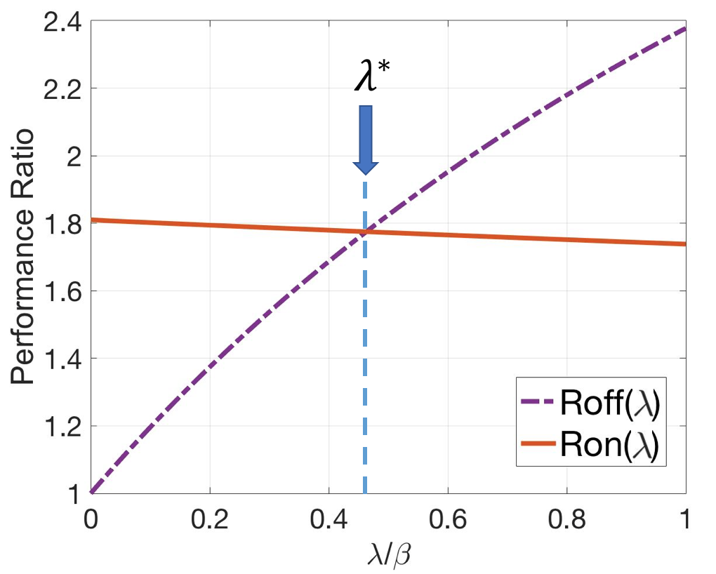
To understand how to find and its corresponding , we consider the example given in Fig. 5. In this example we observe that at , we have . Meanwhile, from Theorem 1 we know that is always a decreasing function and is always an increasing function. Hence, can be computed by finding the intersection of these two functions:
| (18a) | |||||
| (18b) | s.t. | ||||
| (18c) | |||||
| (18d) | |||||
where (18b) ensures the threshold is not larger than the startup cost; otherwise, it is always optimal to turn on the generator. The constraint (18c) ensures that the threshold is within the maximum possible value, and (18d) ensures that we find the threshold that gives us the minimum competitive ratio. We can find the intersection of the two functions by using a simple binary search. As we can see in Fig. 5, by increasing the window size, the value of the threshold over the startup cost () monotonically increases and approaches 1.
Now that the optimal threshold is calculated, we present the competitive ratio of our proposed online algorithm:
Theorem 2.
The competitive ratio of the algorithm CHASEpp satisfies
| (19) |
where
| (20) | ||||
which is and monotonically increases from to as increases.

Proof.
Refer to Appendix B. ∎
If there is no prediction (), we have , and (19) reduces to the competitive ratio of CHASE. Meanwhile, if is large, (20) turns to
| (21) | ||||
One can see that by increasing the value of or , value of the function keeps increasing thus, the competitive ratio keeps decreasing. To understand how the new algorithm improves the competitive ratio of CHASElk, we compare with presented in (11). One can see that in , the term denoted as is larger than the corresponding part in in (11) by . This means that the competitive ratio decreases twice faster with respect to than the previous algorithm. Therefore, our new algorithm always achieves better competitive ratio than the state-of-the-art algorithm CHASElk as much as improvement as shown in Fig. 10 to be discussed later.
Note that from the definition, maximum value of is , which is the competitive ratio of the algorithm that only uses the external supply. Hence, when , it means that instead of using our algorithm it is better to never turn on the generator. We summarize this result in Algorithm 2 denoted as .
Corollary 1.
The competitive ratio of satisfies
| (22) |
By the same logic can be defined. In the rest of this paper, we evaluate the performance of these new algorithms. In Fig. 6, this competitive ratio is depicted as a function of and . When is large, it means the economic advantage of using local generation over external sources is small. Hence, both online and offline algorithms tend to use local generation less often. This improves the competitiveness of online algorithms. Thus, by increasing from to , the competitive ratio decreases from to monotonically.
7. Multiple Generator Scenario
In this section, we solve the multi-generator MCMP problem presented in Sec. 3, where we have N units of heterogeneous generators. Without loss of generality, we assume that . The key is to slice the demand into multiple layers, assign each sub-demand to a different generator, and solve an optimization problem for a single generator. For partitioning, we start from the bottom up, and we slice the demand such that the -th layer has at most units of electricity demand and units of heat demand. Once we used all the local generation capacities, for the remaining demands , we use the external sources. In this way, the bottom layers have the least frequent variations of demand, and we assign these layers to the generators with larger capacities. As a result, we use fewer generators, and these generators observe less variations, which helps to reduce the startup cost. The following theorem captures the performance of offline and online algorithms.
Theorem 3.
The offline algorithm that uses the layering approach produces an optimal offline solution for MCMP, and the online algorithm achieves the following competitive ratio:
| (23) |
where , and is defined in Theorem 2 .
Proof.
Refer to Appendix C. ∎

In the heterogeneous setting, each generator has its own unique prediction-aware online algorithm with a different optimal threshold that depends on their generation capacity . The significance of this result is that it extends the applicability of our online algorithm beyond the homogeneous setting.
8. Lower bound of the Competitive Ratio


Theorem 4.
Let be the length of each time slot. As goes to zero and the discrete time setting approaches to the continues time setting, the competitive ratio for any prediction-aware deterministic online algorithm for is lower bounded by
| (24) |
where is an optimal objective of an optimization problem with system parameters as input.
Proof.
Refer to Appendix D. ∎
Sketch of Proof.
The key idea is that given any deterministic online algorithm , we progressively construct a particular worst-case input , that for the performance ratio we have
| (25) |
In what follows, we explain this input, and it’s corresponding lower bound in Lemma 1. Consider an example of the input in Fig. 8. Starting from the beginning , by giving a large value of differential cost (), the adversary tries to encourage the algorithm to turn on the generator. As soon as the algorithm turns on the generator at , the adversary starts to hurt the algorithm as hard as possible by giving it . Hence, the function keeps decreasing until the algorithm turns off the generator at time . We denote the performance ratio for this input as . One can see that at the beginning, the adversary gives a larger differential cost () as the input. As time goes by and the offline cost changes, the adversary continues by giving a smaller differential cost as input.
Lemma 1.
The lower bound of the competitive ratio is
| (26) |
where is given by
| (27) |
and is given by
| (28) |
Proof.
Refer to Appendix D.1. ∎
Similar to Theorem 1, we find that maximizes the lower bound . First, for each , we find a corresponding such that . This reduces to a single variable function of . Now we find the maximum of the minimum of two single variable functions. We know that for , we have , and is an increasing function. Hence, similar to (18) we keep increasing until we find the intersection of the two functions. Therefore, we always have and , which completes the proof. ∎
In Fig. 8, we plot for different window sizes. As we can see, by increasing the window size, both and keep decreasing. As a result, the lower bound, which is a function of , keeps decreasing.
9. NUMERICAL EXPERIMENTS


We carry out numerical experiments using real-world traces to evaluate the performance of CHASEpp. We calculate the cost incurred by using only external electricity, heating, and wind energy (when no generator is utilized) as a benchmark, and we report the cost reduction of different algorithms compared to this benchmark. We compare performance of the optimal offline algorithm , , , , and , which is a popular algorithm widely used in the control literature (Kwon and Pearson 1977), with both perfect and noisy prediction. The length of each time slot is 1 hour and the total cost incurred during one week (T = 168) is reported.
9.1. Experiment Setting
We obtain the electricity and heat demand traces from (Commission 2021), which belongs to a college in San Francisco, with yearly electricity consumption of around , and gas consumption of around therms. We use wind power traces from (National Renewable Energy Laboratory 2021), which are collected from a wind farm outside San Francisco with an installed capacity of . We obtain the electricity and natural gas price from PG&E (Pacific Gas & Electric Company 2021), and we deploy generators with the same specifications as the one in (Tecogen 2021), with heat recovery efficiency set to be . The incremental cost and running cost per unit time are set to be and respectively. We consider a heating system with the unit heat generation cost of , according to (Green Energy UK 2021) and the startup cost is set to be . The peak for the electricity demand is , so we adopt generators with maximum capacity , , and to fully satisfy the demand. All the experiments are modeled and implemented in Matlab (MATLAB 2021) using Gurobi optimization tools (Gurobi Optimization, LLC 2022).
9.2. Theoretical Ratio


In Fig. 10, we plot the competitive ratio improvement of our algorithm over as a function of and . We can see that our algorithm improves the competitive ratio by up to . As expected by decreasing the value of , or increasing the window size, the competitive ratio improvement increases. But if we keep increasing the window size, both competitive ratios approach , and the competitive ratio gap starts to decrease. In a similar figure, the competitive ratio lower bound is depicted in Fig. 10. We can see that when approaches 0, the lower bound approaches , which is the lower bound of the prediction-oblivious CHASE. We also plot the competitive ratio and the lower bound for different values of in Fig. 12. Our algorithm’s competitive ratio is always better than the previous algorithm, and it is not far from the lower bound. With a 3-hour prediction, our algorithm’s competitive ratio is away from the lower bound by . In the worst case with hours, our algorithm is away by at most . One should note that in practice, 3 hours is a more typical prediction window size (Santhosh et al. 2020).
9.3. The Effect of Prediction Window
In this section, we change the window size from to , and we show the results in Fig. 12. We observe that when the window size is large, all the algorithms perform very well and approach the optimal offline solution. On the other hand, when the window size is small, RHC performs very poorly while our online algorithm performs better than the previous algorithm. It is important to note that depending on the input structure, there may be a large performance discrepancy between and . In the following section, we show how our new online algorithm can improve the previous algorithm’s performance by exploiting the structure of the predicted information.
Effect of the cumulative differential cost: In this section, we build two inputs and depict the cost reduction of the two algorithms for these inputs in Fig. 14 and Fig. 14. We observe that in the first input shown in Fig. 14 with when reaches zero the cumulative differential cost in the window is large, and hence both algorithms turn on the generator, and they have the same performance. On the other hand, in the second input shown in Fig. 14 with when reaches zero the cumulative differential cost is small, and the new algorithm does not turn on the generator and will not spend the additional startup cost, which leads to its better performance. Therefore, for a general input, if we have a large value of demand coming in every time slot, both algorithms perform very well. But if the demand is small , the cumulative differential cost is also small, and using our new algorithm significantly improves the performance.


9.4. The Effect of Prediction Error
While the day-ahead electricity demand prediction has an error range of , the highly fluctuating nature of the wind power makes the next hour’s prediction error to usually be around (Wang and Li 2018). Therefore, it is important to see how the prediction error can affect our online algorithm’s performance. We obtain real-world wind power forecasting error distributions from (Hodge et al. 2012b), where the mean and standard deviation of the errors are based on the typical forecasts in the U.S., and hyperbolic distribution is used to represent the error. In (Hodge et al. 2012a) it has been shown that hyperbolic distribution is superior to the normal distribution in capturing wind power forecasting error. Still, to compare these two, we generate wind power forecasting errors from both. We start with the real-world hyperbolic distribution and zero-mean Gaussian, and in each time slot, we add the errors to the actual values. We also increase the standard deviation by to of the total installed capacity and the total peak demand for the wind power error and the heat demand error, respectively. In Fig. 18 and 18, we report the average cost reduction of the algorithms over runs for two different lookahead window sizes of and hours with Gaussian errors. In Fig. 18 and 18 the results of the simulation for the real-world prediction errors with hyperbolic distribution are shown. It is important to note that for a -hour prediction window size the errors are often in range (Wang and Li 2018). Therefore, by increasing the standard deviation up to , we are stress-testing the algorithm. When is small, both algorithms are robust to the prediction error. When the window size increases, however, the previous algorithm becomes more sensitive, and its performance starts deteriorating. Because, for a large window size, the prediction error of each time slot aggregates over the window, and if the window size becomes too large, the prediction can even worsen the algorithm’s performance. On the other hand, the new online algorithm keeps its performance even for large prediction errors. The reason is that instead of only detecting the segment type, our algorithm checks the cumulative differential cost and only turns on the generator when it sees enough benefits in the look-ahead window.


10. Conclusion and Future Work
We investigate how to leverage the prediction of the near future for online energy generation scheduling in microgrids. We tackle this problem from a new perspective and propose an effective online algorithm design that is fundamentally different from the existing algorithms. Our novel threshold-based online algorithm attains the best competitive ratio to date, which is upper-bounded by , where is the prediction window size. We also characterize a non-trivial lower bound of the competitive ratio and show that the competitive ratio of our algorithm is only away from the lower bound, when a few hours of prediction is available. Our theoretical and empirical evaluations demonstrate that our online algorithm outperforms the state-of-the-art ones. An interesting future direction is to exploit our new design space in developing competitive algorithms for general MTS problems with limited prediction. We also plan to incorporate energy storage system into the problem setting and algorithm design.
11. Acknowledgement
The work presented in this paper was supported in part by a Start-up Grant from School of Data Science (Project No. 9380118), City University of Hong Kong, and a General Research Fund from Research Grants Council, Hong Kong (Project No. CityU 11206821).
References
- (1)
- Blum and Burch (2000) Avrim Blum and Carl Burch. 2000. On-line learning and the metrical task system problem. Machine Learning 39, 1 (2000), 35–58.
- Borodin and El-Yaniv (2005) Allan Borodin and Ran El-Yaniv. 2005. Online computation and competitive analysis. Cambridge University Press.
- Cao and Liu (2018) Xuanyu Cao and KJ Ray Liu. 2018. On the time-varying constraints and bandit feedback of online convex optimization. In 2018 IEEE International Conference on Communications (ICC). IEEE, 1–6.
- Cao et al. (2018) Xuanyu Cao, Junshan Zhang, and H Vincent Poor. 2018. A virtual-queue-based algorithm for constrained online convex optimization with applications to data center resource allocation. IEEE Journal of Selected Topics in Signal Processing 12, 4 (2018), 703–716.
- Carrión and Arroyo (2006) Miguel Carrión and José M Arroyo. 2006. A computationally efficient mixed-integer linear formulation for the thermal unit commitment problem. IEEE Transactions on power systems 21, 3 (2006), 1371–1378.
- Chang et al. (2013) Tsung-Hui Chang, Mahnoosh Alizadeh, and Anna Scaglione. 2013. Real-time power balancing via decentralized coordinated home energy scheduling. IEEE Transactions on Smart Grid 4, 3 (2013), 1490–1504.
- Chen et al. (2015) Niangjun Chen, Anish Agarwal, Adam Wierman, Siddharth Barman, and Lachlan L.H. Andrew. 2015. Online Convex Optimization Using Predictions. SIGMETRICS Perform. Eval. Rev. 43, 1 (2015), 191–204.
- Chen et al. (2016) Niangjun Chen, Joshua Comden, Zhenhua Liu, Anshul Gandhi, and Adam Wierman. 2016. Using predictions in online optimization: Looking forward with an eye on the past. ACM SIGMETRICS Performance Evaluation Review 44, 1 (2016), 193–206.
- Chen and Chang (1995) Po-Hung Chen and Hong-Chan Chang. 1995. Large-scale economic dispatch by genetic algorithm. IEEE transactions on power systems 10, 4 (1995), 1919–1926.
- Chen et al. (2013) Shengbo Chen, Ness B Shroff, and Prasun Sinha. 2013. Heterogeneous delay tolerant task scheduling and energy management in the smart grid with renewable energy. IEEE Journal on Selected Areas in Communications 31, 7 (2013), 1258–1267.
- Coester and Koutsoupias (2018) Christian Coester and Elias Koutsoupias. 2018. The Online -Taxi Problem. arXiv:1807.06645 [cs.DS]
- Commission (2021) California Energy Commission. 2021. California Commercial End-Use Survey. https://www.energy.ca.gov/data-reports/surveys/california-commercial-end-use-survey [Online].
- Fiorini and Aiello (2019) Laura Fiorini and Marco Aiello. 2019. Energy management for user’s thermal and power needs: A survey. Energy Reports 5 (11 2019), 1048–1076.
- Gaing (2003) Zwe-Lee Gaing. 2003. Particle swarm optimization to solving the economic dispatch considering the generator constraints. IEEE transactions on power systems 18, 3 (2003), 1187–1195.
- Green Energy UK (2021) Green Energy UK. 2021. Gas and Electricity Price Quote. https://www.greenenergyuk.com/quote [Online].
- Guan et al. (2003) Xiaohong Guan, Qiaozhu Zhai, and Alex Papalexopoulos. 2003. Optimization based methods for unit commitment: Lagrangian relaxation versus general mixed integer programming. In 2003 IEEE Power Engineering Society General Meeting (IEEE Cat. No. 03CH37491), Vol. 2. IEEE, 1095–1100.
- Guo et al. (2013) Yuanxiong Guo, Miao Pan, Yuguang Fang, and Pramod P Khargonekar. 2013. Decentralized coordination of energy utilization for residential households in the smart grid. IEEE transactions on smart grid 4, 3 (2013), 1341–1350.
- Gurobi Optimization, LLC (2022) Gurobi Optimization, LLC. 2022. Gurobi Optimizer Reference Manual.
- Hajiesmaili et al. (2016) Mohammad H Hajiesmaili, Chi-Kin Chau, Minghua Chen, and Longbu Huang. 2016. Online microgrid energy generation scheduling revisited: The benefits of randomization and interval prediction. In Proceedings of the Seventh International Conference on Future Energy Systems. 1–11.
- Hodge et al. (2012b) Bri-Mathias Hodge, Debra Lew, Michael Milligan, Hannele Holttinen, S Sillanpaa, Emilio Gómez-Lázaro, Richard Scharff, L Soder, Xiaoli Guo Larsén, Gregor Giebel, et al. 2012b. Wind power forecasting error distributions: An international comparison. Technical Report. National Renewable Energy Lab, Golden, CO (United States).
- Hodge et al. (2012a) Bri-Mathias S Hodge, Erik G Ela, and Michael Milligan. 2012a. Characterizing and modeling wind power forecast errors from operational systems for use in wind integration planning studies. Wind Engineering 36, 5 (2012), 509–524.
- Huang et al. (2014) Yingsong Huang, Shiwen Mao, and R Mark Nelms. 2014. Adaptive electricity scheduling in microgrids. IEEE Transactions on Smart Grid 5, 1 (2014), 270–281.
- Irani et al. (2003) Sandy Irani, Sandeep K. Shukla, and Rajesh K. Gupta. 2003. Online strategies for dynamic power management in systems with multiple power-saving states. ACM Trans. Embed. Comput. Syst. 2, 3 (2003), 325–346.
- Kazarlis et al. (1996) Spyros A Kazarlis, AG Bakirtzis, and Vassilios Petridis. 1996. A genetic algorithm solution to the unit commitment problem. IEEE transactions on power systems 11, 1 (1996), 83–92.
- Kroposki (2017) Benjamin Kroposki. 2017. Integrating high levels of variable renewable energy into electric power systems. Journal of Modern Power Systems and Clean Energy 5, 6 (2017), 831–837.
- Kwon and Pearson (1977) Wook Hyun Kwon and Allan E Pearson. 1977. A modified quadratic cost problem and feedback stabilization of a linear system. IEEE Trans. Automat. Control 22, 5 (1977), 838–842.
- Li et al. (2018a) Jie Li, Yikui Liu, and Lei Wu. 2018a. Optimal Operation for Community-Based Multi-Party Microgrid in Grid-Connected and Islanded Modes. IEEE Transactions on Smart Grid 9, 2 (2018), 756–765. https://doi.org/10.1109/TSG.2016.2564645
- Li et al. (2018b) Yingying Li, Guannan Qu, and Na Li. 2018b. Online Optimization with Predictions and Switching Costs: Fast Algorithms and the Fundamental Limit. arXiv:1801.07780
- Li et al. (2020) Zhongwen Li, Zhiping Cheng, Jing Liang, Jikai Si, Lianghui Dong, and Shuhui Li. 2020. Distributed Event-Triggered Secondary Control for Economic Dispatch and Frequency Restoration Control of Droop-Controlled AC Microgrids. IEEE Transactions on Sustainable Energy 11, 3 (2020), 1938–1950.
- Lin et al. (2012) Minghong Lin, Zhenhua Liu, Adam Wierman, and Lachlan L. H. Andrew. 2012. Online algorithms for geographical load balancing. In 2012 International Green Computing Conference (IGCC). 1–10. https://doi.org/10.1109/IGCC.2012.6322266
- Lin et al. (2011) Minghong Lin, Adam Wierman, Lachlan L. H. Andrew, and Eno Thereska. 2011. Dynamic right-sizing for power-proportional data centers. In 2011 Proceedings IEEE INFOCOM. 1098–1106. https://doi.org/10.1109/INFCOM.2011.5934885
- Lin et al. (2020) Yiheng Lin, Gautam Goel, and Adam Wierman. 2020. Online Optimization with Predictions and Non-Convex Losses. Proc. ACM Meas. Anal. Comput. Syst. 4, 1, Article 18 (May 2020), 32 pages.
- Lu et al. (2013) Lian Lu, Jinlong Tu, Chi-Kin Chau, Minghua Chen, and Xiaojun Lin. 2013. Online energy generation scheduling for microgrids with intermittent energy sources and co-generation. ACM SIGMETRICS Performance Evaluation Review 41, 1 (2013), 53–66.
- MATLAB (2021) MATLAB. 2021. version 9.10.0 (R2021a). The MathWorks Inc.
- Menati and Xie (2021) Ali Menati and Le Xie. 2021. A Preliminary Study on the Role of Energy Storage and Load Rationing in Mitigating the Impact of the 2021 Texas Power Outage. In 2021 North American Power Symposium (NAPS). IEEE, 1–5.
- Narayanaswamy et al. (2012) Balakrishnan Narayanaswamy, Vikas K Garg, and TS Jayram. 2012. Online optimization for the smart (micro) grid. In Proceedings of the 3rd international conference on future energy systems: where energy, computing and communication meet. 1–10.
- National Renewable Energy Laboratory (2021) National Renewable Energy Laboratory. 2021. National Wind Technology Center’s Information Portal. http://wind.nrel.gov [Online].
- Neely (2010) Michael J Neely. 2010. Stochastic network optimization with application to communication and queueing systems. Synthesis Lectures on Communication Networks 3, 1 (2010), 1–211.
- Pacific Gas & Electric Company (2021) Pacific Gas & Electric Company. 2021. Rate Information. http://www.pge.com/nots/rates/tariffs/rateinfo.shtml [Online].
- Padhy (2004) Narayana Prasad Padhy. 2004. Unit commitment-a bibliographical survey. IEEE Transactions on power systems 19, 2 (2004), 1196–1205.
- Santhosh et al. (2020) Madasthu Santhosh, Chintham Venkaiah, and DM Vinod Kumar. 2020. Current advances and approaches in wind speed and wind power forecasting for improved renewable energy integration: A review. Engineering Reports 2, 6 (2020), e12178.
- Selvakumar and Thanushkodi (2007) A Immanuel Selvakumar and K Thanushkodi. 2007. A new particle swarm optimization solution to nonconvex economic dispatch problems. IEEE transactions on power systems 22, 1 (2007), 42–51.
- Shi et al. (2018) Ming Shi, Xiaojun Lin, Sonia Fahmy, and Dong-Hoon Shin. 2018. Competitive Online Convex Optimization with Switching Costs and Ramp Constraints. In IEEE INFOCOM 2018 - IEEE Conference on Computer Communications. 1835–1843.
- Shi et al. (2019) Ming Shi, Xiaojun Lin, and Lei Jiao. 2019. On the Value of Look-Ahead in Competitive Online Convex Optimization.
- Shi et al. (2021) Ming Shi, Xiaojun Lin, and Lei Jiao. 2021. Combining regularization with look-ahead for competitive online convex optimization. In IEEE INFOCOM 2021-IEEE Conference on Computer Communications. IEEE, 1–10.
- Snyder et al. (1987) Walter L Snyder, H David Powell, and John C Rayburn. 1987. Dynamic programming approach to unit commitment. IEEE Transactions on Power Systems 2, 2 (1987), 339–348.
- Takriti et al. (1996) Samer Takriti, John R Birge, and Erik Long. 1996. A stochastic model for the unit commitment problem. IEEE Transactions on Power Systems 11, 3 (1996), 1497–1508.
- Tecogen (2021) Tecogen. 2021. Cogeneration Product Data. https://www.tecogen.com/resources?media=product-data [Online].
- Tu et al. (2013) Jinlong Tu, Lian Lu, Minghua Chen, and Ramesh K Sitaraman. 2013. Dynamic provisioning in next-generation data centers with on-site power production. In Proceedings of the fourth international conference on Future energy systems. 137–148.
- Urgaonkar et al. (2011) Rahul Urgaonkar, Bhuvan Urgaonkar, Michael J Neely, and Anand Sivasubramaniam. 2011. Optimal power cost management using stored energy in data centers. In Proceedings of the ACM SIGMETRICS joint international conference on Measurement and modeling of computer systems. 221–232.
- Wang and Li (2018) Jujie Wang and Yaning Li. 2018. Multi-step ahead wind speed prediction based on optimal feature extraction, long short term memory neural network and error correction strategy. Applied Energy 230 (2018), 429–443.
- Yang et al. (2018) Jingjie Yang, Bingqing Guo, and Bo Qu. 2018. Economic optimization on two time scales for a hybrid energy system based on virtual storage. Journal of Modern Power Systems and Clean Energy 6, 5 (2018), 1004–1014.
- Zhang et al. (2016) Ying Zhang, Mohammad H Hajiesmaili, Sinan Cai, Minghua Chen, and Qi Zhu. 2016. Peak-aware online economic dispatching for microgrids. IEEE transactions on smart grid 9, 1 (2016), 323–335.
- Zinkevich (2003) Martin Zinkevich. 2003. Online convex programming and generalized infinitesimal gradient ascent. In Proceedings of the 20th international conference on machine learning (icml-03). 928–936.
Appendix A Proof of Theorem 1
Proof.
Without loss of generality let us consider that in a type 1 critical segment the algorithm turns on the generator at time , where and . and gives us the case that we turn on the generator at . Here we first consider the case with , and then we extend the result to the general . In the case with we turn on the generator at time which means we keep the generator off from to , where .
We denote the outcome of by , and the outcome of the optimal offline algorithm by . Let us define as the set of indices of type- critical segments i.e.,
Denote the sub-cost for type- by
| (29) |
Hence, . We prove by comparing the sub-cost for each type-.
(Type-0): Note that both for all . Hence,
| (30) |
(Type-1): Based on the definition of critical segment, we recall that there is an auxiliary point , such that either ( and ) or ( and ). We assumed we turn on the generator at . Now we focus on the segment . We observe
| (31) |
We consider a particular type-1 critical segment: . Note that by the definition of type-1, at the beginning of this segment for both online and offline algorithms the generator status is off . For the offline algorithm switches from to at time , while for the online algorithm switches at time , both incurring startup cost . Hence, in the interval , the online and offline algorithms have a different status, while in the interval they have the same status. The cost difference between and within is
| (32) |
where .
If we repeat this process for all type-1 critical segments, and we have type-1 critical segments, we obtain
| (33) |
(Type-2) and (Type-3): Now, we repeat the same process for type-2 and type-3 (type-end) critical segments. Let the number of type- critical segments be . We derive similarly for or as
| (34) |
where .
Note that for all . Furthermore, we note , because it takes equal numbers of critical segments for increasing from to 0 and for decreasing from 0 to . We obtain
| (35) |
It should be noted that in the calculation a type-3 critical segment is exactly the same as a type-2 critical segment and hence in the rest of the calculation we just consider type-2 critical segments. As a result we can write for the ease of calculation. We have
| (36) |
By Lemma 2, and Lemma 3 and simplifications, we obtain:
| (37) |
We denote this value as . This is the performance ratio for the case with . Now if we increase , by using the same process we can see that both online and offline cost increase. Using the result from Lemma 4, if we change to general , the increment ratio is as follows:
| (38) |
We denote this ratio as . If this ratio is larger than the previous one , then by increasing , the value of the performance ratio keeps increasing and when goes to , this competitive ratio goes to . On the other hand, if , by increasing the value of , value of the competitive ratio will not increase and is still upper bounded by . This shows that the competitive ratio is upper bonded by the maximum of , and . In Lemma 5 we show that is always an increasing function while is always a decreasing function. This completes the proof. ∎
A.1. Proof of Lemma 2
Lemma 2.
For the (type-1), we have
| (39) |
Proof.
Consider a particular type-1 segment . We denote its offline cost as . We have:
| (40) |
By (Lu et al. 2013, Lemma. 4) and simplification we obtain
| (41) |
Now we need to find the lower bound of both and in the following two steps.
Step 1: We write the lower bound of as follows:
Step 2: To find the lower bound of the length of the interval , we have two cases with or we calculate the lower bound as follows:
Case 1: If , we can see that has two part as and . We note that is lower bounded by the steepest descend when , and ,
| (42) |
and for the second part we have which means
| (43) |
Case 2: On the other hand, when , we know the length of the interval is time slot and its cost difference is less than , hence to calculate the total length we have
| (44) | |||
where the last inequality comes from the fact that . We note that is lower bounded by the steepest descend when , and ,
| (45) |
So one can see that in both of these cases we always have
| (46) |
| (47) |
A.2. Proof of Lemma 3
Lemma 3.
For (type-2), we have
| (49) |
Proof.
Consider a particular type-2 segment . We denote its offline cost as . We have:
| (50) |
By (Lu et al. 2013, Lemma. 4) and simplification we obtain
| (51) |
Furthermore, we note that is lower bounded by the steepest descend when ,
| (52) |
A.3. Proof of Lemma 4
Lemma 4.
Consider a window , in the type-1 critical segment. If we have , then the cost of the online algorithm over the cost of the optimal offline algorithm in this window is upper bounded by the following:
| (55) |
Proof.
By (Lu et al. 2013, Lemma. 4) and simplification we know that in a type-1 critical segment for a window with , for the offline cost we have
On the other hand, if in the type-1 critical segment the online keep the generator off in this window, the cost difference between the online and the offline is equal to , which means
| (57) |
Hence we have
| (58) |
This completes the proof. ∎
A.4. Proof of Lemma 5
Lemma 5.
is always a decreasing function of and is always an increasing function of .
Proof.
: To prove that is always a decreasing function first we take the derivative as a function of . To compute the derivative we only consider the maximization part of . The denominator of the function is always positive and the numerator is given by
| (59) |
Note that we have . If the derivative is always negative. If we show that we have in the maximization part of the function which again shows that derivative is negative. To show that for we have , we first take the derivative as a function of and we can see that the denominator of the function is always positive and the numerator is given by
| (60) |
We can see that for value of the derivative is always negative which means that for the maximum value of happens at . This prove that for both cases the derivative is negative and hence is always a decreasing function.
: Now we show that is an increasing function. We take the derivative and we can see that the denominator of the function is always positive and the numerator is given by
| (61) |
which is always positive, and hence is always an increasing function. This completes the proof. ∎
Appendix B Proof of Theorem 2
Appendix C Proof of Theorem 3
Proof.
This theorem includes two parts as follows:
- •
Offline algorithm: As shown in (Lu et al. 2013, Theorem. 5, and 6), when we have homogeneous generators, the offline algorithm that uses the layering approach produces an optimal offline solution for MCMP. For the case with multiple heterogeneous generators, since assigning the bottom layers to the generators with larger capacities minimizes the start-up cost, it can easily be shown that the layering approach also leads to an optimal offline solution. On the other hand, the operational cost does not depend on the capacity , and it is the same for all the generators. Hence, it can be shown that the layering approach produces an offline optimal.
- •
Online algorithm: In this case, each generator is solving its own sub-problem with a given sub-demand. Hence, the competitive ratio of the algorithm is upper bounded by the largest competitive ratio among all generators.
(65) where
(66) Since the competitive ratio is an increasing function of and , we have:
(67)
This completes the proof.
∎
Appendix D Proof of Theorem 4
Proof.
Finding the lower bound of the competitive ratio is equal to constructing an special input such that for any deterministic online algorithm , we have:
| (68) |
In (Lu et al. 2013), it is shown that when we do not have any prediction , the following input gives us the lower bound.
| (69) |
As one can see in this input, as long as the algorithm keeps the generator off, the adversary keeps giving full demand () as the input, and as soon as the algorithm turns off the generator, the adversary starts giving zero demand () as the input. This simple input is designed in a way that it always tries to hurt the algorithm most. In creating the lower bound for the case with perfect prediction, we follow the same logic, but we need to design a different input.
If we keep giving full demand until the algorithm turns on the generator, at some point, we have already given a lot of full demand to the algorithm, and by turning on the generator, the algorithm can enjoy a window of full demand. In this way, we can not really hurt the algorithm. Therefore we need to carefully choose the demand in the future window in a way that it gives the algorithm some incentive to turn on the generator, but at the same time, it does not give it a lot of demand in the coming window to enjoy. By carefully adjusting this demand, we can find the lower bound.
At any time , we need to construct the input of the time , and the algorithm has already decided the generator status for the time . We need to know that for how many consecutive time slots the algorithm kept the generator off. To this end, we define a counter called . This counter will reset anytime we turn on the generator and keeps increasing when the algorithm keeps the generator off. We define it as follows:
| (70) |
where the initial value of we have , and .
We construct the worst-case input as follows:
| (71) |
Now we need to calculate the proper values for and . We use Lemma 1 toward this end.
D.1. Proof of Lemma 1
Proof.
Consider the input shown in Fig. 8. If the algorithm turns on the generator at some point , we can calculate the performance ratio as the online cost over the offline cost as follows:
| (72) |
where . Since we are looking for the lower bound, we find the minimum across all possible values of . We call this value and define it as follows:
| (73) |
By using the same logic in the proof of Theorem 1, if the algorithm does not turn on the generator in , and keeps the generator off, the ratio of the online cost increment over the offline cost increment is
| (74) |
Hence the lower bound can be calculated by finding the minimum of these two values:
| (75) |
This complete the proof of Lemma 1. ∎
Similar to Theorem 1, we want to find that maximizes the lower bound . First, for each , we find a corresponding such that . This reduces to a single variable function of .
| (76a) | |||||
| (76c) | s.t. | ||||
For a given , the function is a concave function of . Therefore we can easily find a corresponding for each . Now both and are a function of , and we find the maximum of the minimum of two single variable functions. We know that for , we have , and is an increasing function. Hence, similar to (18) we keep increasing until we find the intersection of the two functions. Therefore, can be obtained by solving the following optimization problem:
| (77a) | |||||
| (77e) | s.t. | ||||
Therefore, we always have and , which completes the proof of Theorem 4.
∎