跳到论文正文
W Papers独立论文阅读器 arXiv:2205.12077 论文正文 计算阅读时间 · 0%
引用这篇论文根据当前论文元数据生成,正式投稿前建议核对。


License: arXiv.org perpetual non-exclusive license
arXiv:2205.12077v5 [eess.SP] 30 Sep 2022

Asymptotic Analysis of RLS-based Digital Precoder with Limited PAPR in Massive MIMO

Xiuxiu Ma    Abla Kammoun       Ayed M. Alrashdi       Tarig Ballal       Tareq Y. Al-Naffouri    and Mohamed-Slim Alouini    Thanks: X. Ma, A. Kammoun, T. Ballal,T. Y. Al-Naffouri and M. Alouini are with the Division of Computer, Electrical and Mathematical Science & Engineering, King Abdullah University of Science and Technology (KAUST), Thuwal, KSA. A. M. Alrashdi is with the Department of Electrical Engineering, College of Engineering, University of Ha’il, P.O. Box 2440, Ha’il, 81441, Saudi Arabia. E-mails: ({xiuxiu.ma; abla.kammoun; tarig.ahmed;tareq.alnaffouri;slim.alouini}@kaust.edu.sa; am.alrashdi@uoh.edu.sa)
Abstract

This paper focuses on the performance analysis of a class of limited peak-to-average power ratio (PAPR) precoders for downlink multi-user massive multiple-input multiple-output (MIMO) systems. Contrary to conventional precoding approaches based on simple linear precoders such as maximum ratio transmission (MRT) and regularized zero-forcing (RZF), the precoders in this paper are obtained by solving a convex optimization problem. To be specific, these precoders are designed so that the power of each precoded symbol entry is restricted, and the PAPR at each antenna is tunable. By using the Convex Gaussian Min-max Theorem (CGMT), we analytically characterize the empirical distribution of the precoded vector and the joint empirical distribution between the distortion and the intended symbol vector. This allows us to study the performance of these precoders in terms of per-antenna power, per-user distortion power, signal-to-noise and distortion ratio (SINAD), and bit error probability. We show that for this class of precoders, there is an optimal transmit per-antenna power that maximizes the system performance in terms of SINAD and bit error probability.

Index Terms: 
Precoding, limited PAPR, regularized least squares, Convex Gaussian Min-max Theorem, Gaussian processes, asymptotic performance analysis

I Introduction

Massive multiple-input multiple-output (MIMO) systems are recognized among the key enabling technologies for next-generation communication systems[1, 2, 3]. However, there are still major implementation issues to address for massive MIMO systems to be a reality. First, the number of antennas that can be supported is limited by the transceiver’s form factor. In practice, this issue can be handled by moving the operating frequency to mmWave frequency bands [4]. Second, it requires equipping each antenna with a dedicated radio frequency (RF) chain, which allows the pass-band communication signals to be processed in the base-band [5], thereby leading to a prohibitively high cost and power consumption, calling into question the practicality of such systems. One possible solution is to reduce the number of RF chains by employing hybrid-precoding [6, 7]. However, the work in [8] shows that the power consumption of some hybrid precoding architectures still scales with the number of antennas, and proposed as a solution a linear and highly energy efficient reflect-array and transmit-array antennas scheme. Aside from power consumption, it is of interest to control the power of each RF chain allowing for cheap system modules. In light of this observation, the work in [9] proposed a precoder with fewer RF chains that constrains the power of each signal entry to be below a certain threshold.

The proposed precoder in [9] reminds the conventional regularized zero-forcing precoder (RZF) [10], in that it builds on the regularized least squares (RLS) method to minimize a penalty of the residue sum of squares (RSS). The main difference with RZF is that it constrains the absolute value of the precoded vector to not exceed a certain threshold. Referred to as the RLS-based precoder with limited peak-to-average power ratio (PAPR), the precoder in [9] allows for achieving the two sought-for goals, that is a lower number of RF chains together with a limited PAPR, making it possible to use inexpensive power amplifiers.

I-A Contributions and related works

Performance analysis of non-linear precoders. In this paper, we carry out a rigorous, asymptotic characterizaton of the performance of multi-user downlink transmission when an RLS precoder with limited PAPR is employed. More precisely, we study the asymptotic behavior of the per-antenna power, per-user distortion power, signal-to-noise and distortion ratio (SINAD), and bit error probability when the number of antennas and the number of served users grow large at the same pace. A similar problem has been recently studied in [11, 12] where asymptotic expressions for the distortion error and a lower bound on the achievable rate have been derived. Compared to these works, our contribution differs as follows. On a methodological level, while the works in [11, 12] are based on the non-rigorous replica method, the main tool in our work is the recently developed Convex Gaussian Min-max Theorem (CGMT) [13] framework. Using the CGMT, our analysis goes beyond the performance metrics studied in [11, 12]. Particularly, we assume BPSK modulation while [11, 12] rely on Gaussian signaling. Furthermore, we derive accurate characterization of the joint distribution between the transmitted symbol vector and the distortion error. This characterization allows us to analyze the bit error probability and a tight approximation of the SINAD. On an operational level, we derive several insights from our analysis by studying the obtained asymptotic expressions in different regimes describing small numbers of served users or small/large values of the power control parameter. Particularly, we show that the performance of the RLS precoder with limited PAPR is not always better when the transmit per-antenna power increases, for higher transmit power may also imply higher distortion power. In other words, there is an optimal per-antenna transmit power that maximizes the performance in terms of SINAD and bit error probability. It can be achieved by properly setting the power control parameter.

Convex Gaussian Min-max Theorem. The main ingredient of the proof of our main results is the Convex Gaussian Min-max Theorem (CGMT). This framework has been initiated by Stojnic [14] before being formally developed in [13] and [15]. It has been applied to characterize the asymptotic behavior of convex-optimization-based estimators with application to high-dimensional regression problems as well as binary classification problems. In this line, the work in [15] applied the CGMT to quantify the performances of several estimators including the Least Absolute Shrinkage and Selection Operator (LASSO). As far as wireless communications are concerned, the CGMT has been applied to characterize the performance of non-explicit decoders. In this context, under the assumption of real Gaussian channels, the CGMT was used to derive closed-form approximations of the bit error probability of convex-optimization-based decoders termed box relaxation decoders under Binary Phase Shift Keying (BPSK) signaling [16, 17] as well as M-ary Pulse Amplitude Modulation (M-PAM) signaling [18]. All these works have focused on the design of non-linear algorithms from the decoder perspective. The application of the CGMT for the design of non-linear precoders has not, to the best of our knowledge, been studied, which motivates our work.

I-B Paper Organization

In Section II, we introduce the system model and formulate the problem. Then, in Section III we state our main results characterizing the statistics of the precoded vector and the distortion, based on which we get the asymptotic behavior of the studied specifications and performance metrics, namely, the transmit per-antenna power, the per-user distortion power, the received SINAD, and the bit error probability. In Section IV, numerical simulations are provided to confirm the accuracy of our results before concluding the paper in Section V. For the readers’ convenience, the proofs are deferred to Section VI-X.

I-C Notations

For simplicity, we make use of the following notations onwards.

Our work is to characterize the behaviors of the RLS-based precoder with limited PAPR, in the large dimensional regime where m,n→∞m,n\rightarrow\infty with a fixed ratio δ=m/n\delta=m/n, and to keep the notations short we simply write n→∞n\rightarrow\infty. We say that an event ξ\xi holds with probability approaching 11 (w.p.a.1) if limn→∞​ℙ​[ξ]=1\mathrm{lim}_{n\rightarrow\infty}\mathbb{P}[\xi]=1. If a sequence of random variables XnX_{n} converges to a constant XX, we write Xn→PXX_{n}\stackrel{{\scriptstyle P}}{{\rightarrow}}X. For any vector 𝐱\mathbf{x}, we use xix_{i} or [𝐱]i[{\bf x}]_{i} to denote its ii-th element. We also use the notation ∥⋅∥\|\cdot\| to denote the Euclidean norm, and the notation (x)+(x)_{+} to denote max⁡(x,0)\max(x,0). We write f⁡(x)f(x) as O⁡(g⁡(x))O(g(x)) if there are constants MM such that |f⁡(x)|≤M​g​(x)|f(x)|\leq Mg(x) for all xx going to the limiting value in the analysis.

The empirical distribution of a vector 𝐭∈ℝm{\bf t}\in\mathbb{R}^{m} is given by 1m​∑i=1m𝜹ti\frac{1}{m}\sum_{i=1}^{m}\boldsymbol{\delta}_{t_{i}} where 𝜹ti\boldsymbol{\delta}_{t_{i}} is the Dirac delta mass at tit_{i}. For q∈ℕq\in\mathbb{N}, a function f:ℝq→ℝf:\mathbb{R}^{q}\to\mathbb{R} is said to be pseudo-Lipschitz of order kk if for all 𝐱{\bf x} and 𝐲{\bf y} in ℝq\mathbb{R}^{q}, |f⁡(𝐱)−f⁡(𝐲)|≤C⁡(1+‖𝐱‖k−1+‖𝐲‖k−1)​‖𝐱−𝐲‖\left|f({\bf x})-f({\bf y})\right|\leq C(1+\|{\bf x}\|^{k-1}+\|{\bf y}\|^{k-1})\|{\bf x}-{\bf y}\|. The Wasserstein−k-k distance [19] between two measures μ\mu and ν\nu is defined as Wk​(μ,ν)=(infρ𝔼(X,Y)∼ρ​|X−Y|k)1kW_{k}(\mu,\nu)=\left(\inf_{\rho}\mathbb{E}_{(X,Y)\sim\rho}|X-Y|^{k}\right)^{\frac{1}{k}} where the infimum is over all random variables (X,Y)(X,Y) such that X∼μX\sim\mu and Y∼νY\sim\nu marginally. A sequence of probability distributions νp\nu_{p} converges in WkW_{k} to ν\nu if Wk​(νp,ν)→0W_{k}(\nu_{p},\nu)\to 0 as p→∞.p\to\infty. An equivalent definition of the convergence in WkW_{k} is that, for any ff pseudo-Lipschitz of order kk, limp→∞𝔼⁡[f⁡(Xp)]=𝔼⁡[f⁡(X)]\lim_{p\to\infty}\mathbb{E}[f(X_{p})]=\mathbb{E}[f(X)] where the expectation is with respect Xp∼νpX_{p}\sim\nu_{p} and X∼νX\sim\nu.

II System model and problem formulation

Consider a conventional multiuser downlink, slow narrow band transmission between a base station equipped with nn transmit antennas and mm single antenna user terminals. The precoding scheme is a function that maps the user information symbols, collected in 𝐬=[s1,s2,…,sm]T={±1}m\mathbf{s}=[s_{1},s_{2},...,s_{m}]^{T}=\{{\pm}1\}^{m} and assumed to be drawn uniformly from the BPSK constellation, into an nn-dimensional signal 𝐱=[x1,x2,…,xn]T\mathbf{x}=[x_{1},x_{2},...,x_{n}]^{T}. Since the signal here is BPSK, we assume a real wireless channel and additive noise. Letting 𝐡k{\bf h}_{k} denote the channel vector between the base station and user kk, the received signal at the kk-th user writes as

yk=𝐡kT​𝐱+zk,{y}_{k}={\bf h}_{k}^{T}{\bf x}+z_{k}, (1)

where zk{z}_{k} is the additive noise, assumed to follow a Gaussian distribution with mean zero and variance σ2\sigma^{2}. Stacking the received signals into a vector 𝐲=[y1,⋯,ym]T{\bf y}=\left[y_{1},\cdots,y_{m}\right]^{T} yields

𝐲=𝐇𝐱+𝐳,{\bf y}={\bf H}{\bf x}+{\bf z},

where 𝐳=[z1,⋯,zm]T{\bf z}=\left[z_{1},\cdots,z_{m}\right]^{T} and 𝐇=[𝐡1,⋯,𝐡m]T{\bf H}=\left[{\bf h}_{1},\cdots,{\bf h}_{m}\right]^{T}.

The main goal of precoding is to remove the effect of the channel by minimizing the error between the channel-distorted received vector 𝐇𝐱{\bf Hx} and the information vector 𝐬{\bf s}. To meet this requirement, the non-linear least squares precoder proposed in [12] is formulated as the solution to the following regularized least squares problem:

𝐱^=arg⁡min𝐱∈𝕏n⁡‖𝐇𝐱−ρ​𝐬‖2+λ​‖𝐱‖2,\hat{\bf x}=\arg\min_{{\bf x}\in\mathbb{X}^{n}}\|{\bf Hx}-\sqrt{\rho}{\bf s}\|^{2}+\lambda\|{\bf x}\|^{2}, (2)

where ρ{\rho} is a positive power control factor, λ\lambda is a positive regularization parameter and 𝕏\mathbb{X} being a predefined set containing admissible values for the precoded signal. The formulation in (2) defines a whole class of precoded vectors for different choices of the set 𝕏\mathbb{X} and parameter λ\lambda. For example, if 𝕏=ℝ\mathbb{X}=\mathbb{R} and λ>0\lambda>0, we obtain the RZF precoding given by

𝐱^RZF=ρ​(𝐇T​𝐇+λ​𝐈n)−1​𝐇T​𝐬,\hat{\bf x}_{\rm RZF}=\sqrt{\rho}\left({\bf H}^{T}{\bf H}+\lambda{\bf I}_{n}\right)^{-1}{\bf H}^{T}{\bf s},

which for λ=0\lambda=0 reduces to the zero-forcing (ZF) precoding (assuming m>nm>n)

𝐱^ZF=ρ​(𝐇T​𝐇)−1​𝐇T​𝐬.\hat{\bf x}_{\rm ZF}=\sqrt{\rho}\left({\bf H}^{T}{\bf H}\right)^{-1}{\bf H}^{T}{\bf s}.

When 𝕏=[−P,P]\mathbb{X}=[-\sqrt{P},\sqrt{P}], the precoder in (2) does not admit a closed-form expression, characterizing the performance of the precoder is a challenging task. In this paper, we aim to study its performance in the large dimensional regime in which the number of antennas nn and the number of users mm grow large at the same pace. More formally, in our analysis, we rely on the following assumptions.

Assumption 1.

The number of antennas nn and the number of users mm grow to infinity at a fixed ratio δ:=mn\delta:=\frac{m}{n}.

Assumption 2.

The channel matrix 𝐇{\bf H} has independent and identically distributed Gaussian entries with zero mean and a variance equal to 1n\frac{1}{n}.

We are interested in characterizing the performance of the precoder in (2) with respect to the following specifications and performance metrics.

Per-antenna power: We define the per-antenna transmit power as

Pb:=‖𝐱^‖2n.P_{b}:=\frac{\|\hat{\bf x}\|^{2}}{n}. (3)

Per-user distortion error power: By expressing the received signal at user kk as

yk=ρ​sk+𝐡kT​𝐱^−ρ​sk+zk,y_{k}=\sqrt{\rho}{s_{k}}+{\bf h}_{k}^{T}\hat{\bf x}-\sqrt{\rho}{s_{k}}+z_{k}, (4)

the distortion error observed by user kk is represented by the quantity 𝐡kT​𝐱^−ρ​sk{\bf h}_{k}^{T}\hat{\bf x}-\sqrt{\rho}s_{k}. We define the per-user distortion error power as

Pd:=‖𝐇​𝐱^−ρ​𝐬‖2m.P_{d}:=\frac{\|{\bf H\hat{\bf x}}-\sqrt{\rho}{\bf s}\|^{2}}{m}. (5)

Average per-user SINAD: From (4), we can easily see that the SINAD{\rm SINAD} at user kk is given by

SINADk=ρ𝔼sk​|𝐡kT​𝐱^−ρ​sk|2+σ2.{\rm SINAD}_{k}=\frac{\rho}{\mathbb{E}_{s_{k}}\left|{\bf h}_{k}^{T}\hat{\bf x}-\sqrt{\rho}s_{k}\right|^{2}+\sigma^{2}}.

We define the average per user SINAD as:

SINAD¯=1m​∑k=1m𝔼⁡[SINADk].\overline{\rm SINAD}=\frac{1}{m}\sum_{k=1}^{m}\mathbb{E}\left[{\rm SINAD}_{k}\right]. (6)

Average per-user SINAD upper bound and lower bound: From Jensen’s inequality, we can easily check that the expected value of the SINAD at user kk can be upper bounded and lower bounded as

𝔼⁡[SINADk]≤𝔼⁡[ρ|𝐡kT​𝐱^−ρ​sk|2+σ2],\mathbb{E}[{\rm SINAD}_{k}]\leq\mathbb{E}\left[\frac{\rho}{\left|{\bf h}_{k}^{T}\hat{\bf x}-\sqrt{\rho}s_{k}\right|^{2}+\sigma^{2}}\right], (7)
𝔼⁡[SINADk]≥ρ𝔼⁡[|𝐡kT​𝐱^−ρ​sk|2]+σ2.\mathbb{E}[{\rm SINAD}_{k}]\geq\frac{\rho}{\mathbb{E}\left[\left|{\bf h}_{k}^{T}\hat{\bf x}-\sqrt{\rho}s_{k}\right|^{2}\right]+\sigma^{2}}. (8)

From (7) and (8), we can prove that the following quantities define upper and lower bounds for the average per-user SINAD:

SINADup\displaystyle{\rm SINAD}_{\rm up} =1m​∑k=1m𝔼⁡[ρ|𝐡kT​𝐱^−ρ​sk|2+σ2],\displaystyle=\frac{1}{m}\sum_{k=1}^{m}\mathbb{E}\left[\frac{\rho}{|{\bf h}_{k}^{T}\hat{\bf x}-\sqrt{\rho}s_{k}|^{2}+\sigma^{2}}\right], (9)
SINADlb\displaystyle{\rm SINAD}_{\rm lb} =ρ𝔼⁡[1m​∑k=1m|𝐡kT​𝐱^k−ρ​sk|2]+σ2.\displaystyle=\frac{\rho}{\mathbb{E}\left[\frac{1}{m}\sum_{k=1}^{m}|{\bf h}_{k}^{T}\hat{\bf x}_{k}-\sqrt{\rho}s_{k}|^{2}\right]+\sigma^{2}}. (10)

In practice, we predict the SINAD lower bound in (10) to provide a tight approximation for the SINAD. Indeed, under Assumption 2, all users experience the same channel statistics, we expect that

𝔼sk​|𝐡kT​𝐱^−ρ​sk|2\mathbb{E}_{s_{k}}\left|{\bf h}_{k}^{T}\hat{\bf x}-\sqrt{\rho}s_{k}\right|^{2}

is asymptotically close to 1m​∑k=1m|𝐡kT​𝐱^−ρ​sk|2\frac{1}{m}\sum_{k=1}^{m}\left|{\bf h}_{k}^{T}\hat{\bf x}-\sqrt{\rho}s_{k}\right|^{2}. This latter term should converge to its expectation 𝔼⁡[1m​∑k=1m|𝐡kT​𝐱^−ρ​sk|2]\mathbb{E}\left[\frac{1}{m}\sum_{k=1}^{m}\left|{\bf h}_{k}^{T}\hat{\bf x}-\sqrt{\rho}s_{k}\right|^{2}\right], and hence substituting it by its expectation leads to SINADlb{\rm SINAD}_{\rm lb}. Therefore, in Section IV, we compare the empirical SINAD with our approximation for SINADlb{\rm SINAD}_{\rm lb} and validate its accuracy.

Bit error rate and bit error probability: The bit error rate (BER) is defined as

BER:=1m∑i=1m𝟏{sign(yi)≠si},\mathrm{BER}:=\frac{1}{m}\sum_{i=1}^{m}{\bf 1}_{\{\mathrm{sign}(y_{i})\neq s_{i}\}}, (11)

where 𝟏{⋅}{\bf 1}_{\{\cdot\}} denotes the indicator function. Another related quantity of interest is the bit error probability PeP_{e}, which is defined as the expectation of the BER, i.e.,

Pe:=𝔼[BER]=1m∑i=1mℙ[sign(yi)≠si].P_{e}:=\mathbb{E}[\mathrm{BER}]=\frac{1}{m}\sum_{i=1}^{m}\mathbb{P}[\mathrm{sign}(y_{i})\neq s_{i}]. (12)

Although both the RZF and ZF precoding admit a closed-form expression, the PAPR at each RF chain is not restricted. Taking the definition in [9], the per-antenna PAPR is defined as follows:

𝐏𝐀𝐏𝐑i:=(1J​∑j=1J|xi​(j)|2)−1​maxj∈[J]​|xi​(j)|2,{\mathbf{PAPR}}_{i}:=\left(\frac{1}{J}\sum_{j=1}^{J}|x_{i}(j)|^{2}\right)^{-1}\max_{j\in[J]}|x_{i}(j)|^{2}, (13)

where 𝐱⁡(j){\bf x}(j) is the jj-th realization of the transmit vector, and JJ is the number of samples. We claim that

limJ→∞𝔼⁡[1J​∑j=1J|xi​(j)|2]=limn→∞𝔼⁡[1n​∑i=1n|xi​(j)|2],\lim_{J\to\infty}\mathbb{E}\left[\frac{1}{J}\sum_{j=1}^{J}|x_{i}(j)|^{2}\right]=\lim_{n\to\infty}\mathbb{E}\left[\frac{1}{n}\sum_{i=1}^{n}|x_{i}(j)|^{2}\right], (14)

which means the average PAPR over antennas equals that over time. The above result, verified by simulations, follows because the channel statistics over all antennas are the same, so there is no reason that one antenna experiences more power than any other one. As illustrated later in the following sections, the limiting of the per-antenna power represented by the right-hand side of (14) can be tuned to any target value by properly choosing the power control parameter. Moreover, by construction, the entries of the precoded vector are in the set 𝕏=[−P,P]\mathbb{X}=\left[-\sqrt{P},\sqrt{P}\right], where PP is carefully chosen so that the peak value of the precoded vector is restricted. As a consequence, the studied precoder achieves a PAPR that is less than P/ℰP/\mathcal{E} where ℰ\mathcal{E} is the target power value. (2) will be thus referred to as the RLS-based precoder with limited PAPR and for simplicity termed as limited PAPR-RLS precoder.

III Main results

III-A Distributional characterization of the precoded vector and the distortion error

A major result of our study is the theoretical characterization of the empirical distributions of the elements of the precoded vector 𝐱^\hat{\bf x} and the joint empirical distribution of the distortion error vector given by

𝐞^=(𝐇​𝐱^−ρ​𝐬)\hat{\bf e}=\left({\bf H}\hat{\bf x}-\sqrt{\rho}{\bf s}\right)

and the transmitted symbol 𝐬{\bf s}. As shown next, both of these distributional characterizations will be instrumental in sharply characterizing the convergences of the specifications and performance metrics introduced in the previous section.

Theorem 1 (Distributional characterization of the precoded vector).

Consider the following max-min optimization problem:

ϕ¯=maxβ≥0⁡minτ≥0​τ​β​δ2+ρ​β2​τ−β24+Y⁡(β,τ),\overline{\phi}=\max_{\beta\geq 0}\min_{\tau\geq 0}\frac{\tau\beta\delta}{2}+\frac{\rho\beta}{2\tau}-\frac{\beta^{2}}{4}+Y(\beta,\tau), (15)

where

Y(β,τ)=βα(𝔼H∼𝒩⁡(0,1)[(H−Pα)2𝟏{H≥Pα}]−12),Y(\beta,\tau)=\frac{\beta}{\alpha}\left(\mathbb{E}_{H\sim\mathcal{N}(0,1)}\left[(H-\sqrt{P}\alpha)^{2}{\bf 1}_{\left\{H\geq\sqrt{P}\alpha\right\}}\right]-\frac{1}{2}\right),

with α=1/τ+2​λ/β\alpha=1/\tau+2\lambda/\beta.

  1. (i)

    The optimization problem in (15) admits a unique finite saddle-point (β⋆,τ⋆)(\beta^{\star},\tau^{\star}) if and only if λ>0\lambda>0 or λ=0\lambda=0 and δ>1\delta>1.

  2. (ii)

    When λ=0\lambda=0 and δ>1\delta>1, the saddle point (β⋆,τ⋆)(\beta^{\star},\tau^{\star}) of (15) is given by

    τ⋆\displaystyle\tau^{\star} =arg⁡minτ≥0⁡(τ​δ2+ρ2​τ+Y~​(τ))+2,\displaystyle=\arg\min_{\tau\geq 0}\left(\frac{\tau\delta}{2}+\frac{\rho}{2\tau}+\tilde{Y}(\tau)\right)_{+}^{2}, (16)
    β⋆\displaystyle\beta^{\star} =(τ⋆​δ+ρτ⋆+2​Y~​(τ⋆))+,\displaystyle=\left({\tau^{\star}\delta}+\frac{\rho}{\tau^{\star}}+2\tilde{Y}(\tau^{\star})\right)_{+}, (17)

    where

    Y~(τ):=τ(𝔼[(H−Pτ)2𝟏{H≥Pτ}]−12).\tilde{Y}(\tau):=\tau\left(\mathbb{E}\left[(H-\frac{\sqrt{P}}{\tau})^{2}{\bf 1}_{\{H\geq\frac{\sqrt{P}}{\tau}\}}\right]-\frac{1}{2}\right).

    Moreover, ϕ¯\overline{\phi} reduces to

    ϕ¯=(τ​δ2+ρ2​τ+Y~​(τ))+2.\overline{\phi}=\left(\frac{\tau\delta}{2}+\frac{\rho}{2\tau}+\tilde{Y}(\tau)\right)_{+}^{2}.
  3. (iii)

    Let 𝐱^\hat{\bf x} be the solution of (2), and consider its associated empirical density function

    μ^​(𝐱^):=1n​∑i=1n𝜹𝐱^i.\hat{\mu}(\hat{\bf x}):=\frac{1}{n}\sum_{i=1}^{n}\boldsymbol{\delta}_{\hat{\bf x}_{i}}.

    Further, let the function θ:ℝ→[−P,P]\theta:\mathbb{R}\to[-\sqrt{P},\sqrt{P}],

    θ⁡(γ):={−Pif​γ≤−P​α⋆γα⋆if−P​α⋆≤γ≤P​α⋆Pif​γ≥P​α⋆,\theta(\gamma):=\left\{\begin{array}[]{ll}-\sqrt{P}&\mathrm{if}\gamma\leq-\sqrt{P}\alpha^{\star}\\ \frac{\gamma}{\alpha^{\star}}&\mathrm{if}-\sqrt{P}\alpha^{\star}\leq\gamma\leq\sqrt{P}\alpha^{\star}\\ \sqrt{P}&\mathrm{if}\gamma\geq\sqrt{P}\alpha^{\star}\end{array},\right.

    where α⋆=1/τ⋆+2​λ/β⋆\alpha^{\star}=1/{\tau^{\star}}+2\lambda/\beta^{\star}. Assume either λ>0\lambda>0 or λ=0\lambda=0 and δ>1\delta>1. Then, under Assumption 1 and Assumption 2, for any pseudo-Lipschitz function ff of order kk, it holds that

    1n​∑i=1nf⁡(𝐱^i)→P𝔼H​[f⁡(θ⁡(H))],\frac{1}{n}\sum_{i=1}^{n}f(\hat{\bf x}_{i})\stackrel{{\scriptstyle P}}{{\rightarrow}}\mathbb{E}_{H}\left[f(\theta(H))\right],

    where H∼𝒩⁡(0,1)H\sim\mathcal{N}(0,1). Particularly, the empirical density function μ^​(𝐱^)\hat{\mu}(\hat{\bf x}) converges in Wasserstein−k-k distance to θ⁡(H)\theta(H).

Proof.

See Section VI-C. ∎

Theorem 2 (Distributional characterization of the distortion).

Consider the setting of Theorem 1. Let f:ℝ2→ℝf:\mathbb{R}^{2}\to\mathbb{R} be a pseudo-Lipschitz function of order 22 and let α⋆=1/τ⋆+2​λ/β⋆\alpha^{\star}=1/\tau^{\star}+2\lambda/\beta^{\star}. Assume either λ>0\lambda>0 or λ=0\lambda=0 and δ>1\delta>1. Then, under Assumption 1 and Assumption 2, the following convergence holds true:

1m​∑i=1mf⁡([𝐞^]i,si)→P𝔼H,S​[f⁡(β⋆2​(τ⋆)2​δ−ρ​H−ρ​Sτ⋆​δ,S)],\begin{split}&\frac{1}{m}\sum_{i=1}^{m}f(\left[\hat{\bf e}\right]_{i},s_{i})\\ \stackrel{{\scriptstyle P}}{{\rightarrow}}&\mathbb{E}_{H,S}\left[f\left(\frac{\beta^{\star}}{2}\frac{\sqrt{(\tau^{\star})^{2}\delta-\rho}H-\sqrt{\rho}S}{\tau^{\star}\delta},S\right)\right],\end{split} (18)

where HH is a standard normal scalar variable and SS a discrete binary variable taking 11 and −1-1 with equal probabilities. Equivalently, letting

μ^​(𝐞,𝐬):=1m​∑i=1m𝜹([𝐞]i,si),\hat{\mu}({\bf e},{\bf s}):=\frac{1}{m}\sum_{i=1}^{m}\boldsymbol{\delta}_{([{\bf e}]_{i},s_{i})},

then μ^​(𝐞,𝐬)\hat{\mu}({\bf e},{\bf s}) converges in Wasserstein−2-2 distance to the distribution of (β⋆2​(τ⋆)2​δ−ρ​H−ρ​Sτ⋆​δ,S)(\frac{\beta^{\star}}{2}\frac{\sqrt{(\tau^{\star})^{2}\delta-\rho}H-\sqrt{\rho}S}{\tau^{\star}\delta},S).

Proof.

See Section VI-D. ∎

III-B Characterizations of specifications and performance metrics

As an application of Theorem 1 and Theorem 2, we derive closed-form approximations for the specifications and performance metrics defined in Section II:

Corollary 1 (Convergence of the average SINAD upper and lower bounds).

Consider Assumption 1 and 2, then SINAD¯up\overline{\rm SINAD}_{\rm up} converges to:

SINAD¯up→SINAD¯up⋆:⁣=𝔼H,S​[ρ(β⋆)24​(((τ⋆)2​δ−ρ)​H−ρ​S)2(τ⋆​δ)2+σ2],\begin{split}&\overline{\rm SINAD}_{\rm up}\to\overline{\rm SINAD}_{\rm up}^{\star}\\ :=&\mathbb{E}_{H,S}\left[\frac{\rho}{\frac{(\beta^{\star})^{2}}{4}\frac{\left((\sqrt{(\tau^{\star})^{2}\delta-\rho})H-\sqrt{\rho}S\right)^{2}}{(\tau^{\star}\delta)^{2}}+\sigma^{2}}\right],\end{split} (19)

and SINAD¯lb\overline{\rm SINAD}_{lb} converges to:

SINAD¯lb→PSINAD¯lb⋆:=ρ(β⋆)24​δ+σ2.\overline{\rm SINAD}_{\rm lb}\stackrel{{\scriptstyle P}}{{\rightarrow}}\overline{\rm SINAD}_{\rm lb}^{\star}:=\frac{\rho}{\frac{(\beta^{\star})^{2}}{4\delta}+\sigma^{2}}. (20)
Proof.

Function x↦ρx2+σ2x\mapsto\frac{\rho}{x^{2}+\sigma^{2}} is a Lipschitz function. Applying Theorem 2 yields:

1m​∑k=1mρ|ek|2+σ2→P𝔼H,S​[ρ(β⋆)24​(((τ⋆)2​δ−ρ)​H−ρ​S)2(τ⋆​δ)2+σ2].\begin{split}&\frac{1}{m}\sum_{k=1}^{m}\frac{\rho}{|e_{k}|^{2}+\sigma^{2}}\\ \stackrel{{\scriptstyle P}}{{\rightarrow}}&\mathbb{E}_{H,S}\left[\frac{\rho}{\frac{(\beta^{\star})^{2}}{4}\frac{\left((\sqrt{(\tau^{\star})^{2}\delta-\rho})H-\sqrt{\rho}S\right)^{2}}{(\tau^{\star}\delta)^{2}}+\sigma^{2}}\right].\end{split} (21)

Finally, since x↦ρx2+σ2x\mapsto\frac{\rho}{x^{2}+\sigma^{2}} is bounded by ρσ2\frac{\rho}{\sigma^{2}}, the convergence in (19) follows from the dominated convergence theorem. To prove (20), we use the fact that x↦x2x\mapsto x^{2} is a pseudo-Lipschitz function of order 22. Hence, we may again use Theorem 2 to obtain

1m​∑k=1m|ek|2→P(β⋆)24​δ.\frac{1}{m}\sum_{k=1}^{m}|e_{k}|^{2}\stackrel{{\scriptstyle P}}{{\rightarrow}}\frac{(\beta^{\star})^{2}}{4\delta}.

To prove the convergence in (20), it suffices to check that 1m​∑k=1m|ek|2\frac{1}{m}\sum_{k=1}^{m}|e_{k}|^{2} is bounded. Indeed, if this is true then one can in a similar way as before use the dominated convergence theorem to prove the convergence of the expectation of 1m​∑k=1m|ek|2\frac{1}{m}\sum_{k=1}^{m}|e_{k}|^{2} to its probability limit. Using the fact that 𝐱^\hat{\bf x} minimizes the cost in (2), the following inequality holds:

1m​‖𝐇​𝐱^−ρ​𝐬‖2+λm​‖𝐱^‖2≤1m​‖ρ​𝐬‖2\frac{1}{m}\|{\bf H}\hat{\bf x}-\sqrt{\rho}{\bf s}\|^{2}+\frac{\lambda}{m}\|\hat{\bf x}\|^{2}\leq\frac{1}{m}\|\sqrt{\rho}{\bf s}\|^{2}

and hence,

1m​‖𝐇​𝐱^−ρ​𝐬‖2≤ρ.\frac{1}{m}\|{\bf H}\hat{\bf x}-\sqrt{\rho}{\bf s}\|^{2}\leq\rho.

Recalling that 1m​∑k=1m|ek|2=1m​‖𝐇​𝐱^−ρ​𝐬‖2\frac{1}{m}\sum_{k=1}^{m}|e_{k}|^{2}=\frac{1}{m}\|{\bf H}\hat{\bf x}-\sqrt{\rho}{\bf s}\|^{2} we establish that 1m​∑k=1m|ek|2\frac{1}{m}\sum_{k=1}^{m}|e_{k}|^{2} is bounded. ∎

Corollary 2 (Convergence of the per-antenna power and the per-user distortion error power).

Under the setting of Theorem 1, the per-antenna and the per-user distortion error power satisfy the following convergences:

Pb→PPb⋆:=δ​(τ⋆)2−ρ,P_{b}\stackrel{{\scriptstyle P}}{{\rightarrow}}P_{b}^{\star}:=\delta(\tau^{\star})^{2}-\rho, (22)

and

Pd→PPd⋆:=(β⋆)24​δ.P_{d}\stackrel{{\scriptstyle P}}{{\rightarrow}}P_{d}^{\star}:=\frac{(\beta^{\star})^{2}}{4\delta}. (23)
Proof.

Note that Pd=1m​∑k=1m|ek|2P_{d}=\frac{1}{m}\sum_{k=1}^{m}|e_{k}|^{2}. The convergence of PdP_{d} to its probability limit has been established in the proof of Corollary 20. The convergence of PbP_{b} to the limit in (22) follows directly by applying Theorem 1 along with the first-order optimality condition for the variable τ\tau. ∎

Corollary 23 allows us to provide an interpretation of the parameters τ⋆\tau^{\star} and β⋆\beta^{\star}. From the convergences stated in this Corollary, it appears that τ⋆\tau^{\star} is related to how much power is devoted to the precoded vector 𝐱^\hat{\bf x}, while β⋆\beta^{\star} allows for quantifying the amount of distortion experienced by the PAPR precoder. The control factor ρ\rho can always be adjusted to fix the power Pb⋆P_{b}^{\star} to a given feasible value. However, this would lead to varying the coefficient β⋆\beta^{\star} which determines the distortion level. More details on the role of the control factor ρ\rho on the performance will be given in this section and in section IV.

Corollary 3 (Convergence of the bit error probability).

Under the setting of Theorem 1, the bit error probability defined in (12) converges to

Pe→Pe⋆:=Q⁡(ρ−β⋆​ρ2​τ⋆​δ(β⋆)24​(τ⋆)2​δ−ρ(τ⋆)2​δ2+σ2).P_{e}{\to}P_{e}^{\star}:=Q\left(\frac{\sqrt{\rho}-\frac{\beta^{\star}\sqrt{\rho}}{2\tau^{\star}\delta}}{\sqrt{\frac{(\beta^{\star})^{2}}{4}\frac{(\tau^{\star})^{2}\delta-\rho}{(\tau^{\star})^{2}\delta^{2}}+\sigma^{2}}}\right).
Proof.

The symbol sks_{k} is decoded erroneously if

𝐡kT​𝐱^−ρ+zk≤−ρ{\bf h}_{k}^{T}\hat{\bf x}-\sqrt{\rho}+z_{k}\leq-\sqrt{\rho}

when sk=1s_{k}=1 and

𝐡kT​𝐱^+ρ+zk≥ρ{\bf h}_{k}^{T}\hat{\bf x}+\sqrt{\rho}+z_{k}\geq\sqrt{\rho}

when sk=−1s_{k}=-1. So

Pe=12​ℙ​[𝐡kT​𝐱^−ρ​sk+zk≤−ρ|sk=1]+12​ℙ​[𝐡kT​𝐱^−ρ​sk+zk≥ρ|sk=−1].\begin{split}P_{e}&=\frac{1}{2}\mathbb{P}\left[{\bf h}_{k}^{T}\hat{\bf x}-\sqrt{\rho}s_{k}+z_{k}\leq-\sqrt{\rho}\ |\ s_{k}=1\right]\\ &+\frac{1}{2}\mathbb{P}\left[{\bf h}_{k}^{T}\hat{\bf x}-\sqrt{\rho}s_{k}+z_{k}\geq\sqrt{\rho}|s_{k}=-1\right].\end{split} (24)

Using Theorem 2 along with the Portemanteau Lemma [20], we prove that

Pe→\displaystyle P_{e}\to
12​ℙ​[β⋆2​(τ⋆)2​δ−ρ​H−ρ​Sτ⋆​δ+σ​Z≤−ρ|S=1]\displaystyle\frac{1}{2}\mathbb{P}\left[\frac{\beta^{\star}}{2}\frac{\sqrt{(\tau^{\star})^{2}\delta-\rho}H-\sqrt{\rho}S}{\tau^{\star}\delta}+\sigma Z\leq-\sqrt{\rho}|S=1\right]
+\displaystyle+ 12​ℙ​[β⋆2​(τ⋆)2​δ−ρ​H−ρ​Sτ⋆​δ+σ​Z≥ρ|S=−1]\displaystyle\frac{1}{2}\mathbb{P}\left[\frac{\beta^{\star}}{2}\frac{\sqrt{(\tau^{\star})^{2}\delta-\rho}H-\sqrt{\rho}S}{\tau^{\star}\delta}+\sigma Z\geq\sqrt{\rho}|S=-1\right] (25)
=\displaystyle= Q⁡(ρ−β⋆​ρ2​τ⋆​δ(β⋆)24​(τ⋆)2​δ−ρ(τ⋆)2​δ2+σ2).\displaystyle Q\left(\frac{\sqrt{\rho}-\frac{\beta^{\star}\sqrt{\rho}}{2\tau^{\star}\delta}}{\sqrt{\frac{(\beta^{\star})^{2}}{4}\frac{(\tau^{\star})^{2}\delta-\rho}{(\tau^{\star})^{2}\delta^{2}}+\sigma^{2}}}\right). (26)

where in (25) ZZ follows a standard normal distribution with mean zero and variance 11. ∎

It is important to note that although a BPSK modulation is assumed, (26) is different from the asymptotic bit error probability Pe=Q⁡(2​SNR){P_{e}}=Q(\sqrt{2{\rm SNR}}). The reason lies in the fact that the latter relation holds in the case of additive Gaussian noise that is independent of the transmitted symbols. In our case, we have not only noise but also the distortion 𝐞^\hat{\bf e} which is correlated with the transmitted symbols, as evidenced by Theorem 2.

III-C Special cases: RZF and ZF precoding (P→∞P\to\infty)

The analysis of the RZF and ZF precoding in multi-user downlink systems has been the focus of several studies in the literature. Among these studies, we cite the work in [21] which considered this problem with sophisticated channel models involving different correlations across users. However, to the best of our knowledge, none of the existing works studied the bit error probability approximation (all the focus being on the asymptotic characterization of the SINAD). In the sequel, we show that by taking P→∞P\to\infty in the asymptotic expressions of Theorem 1, we can simplify the expression (20) to reach the same results for the asymptotic SINAD performance obtained in the literature. Additionally, we obtain new asymptotic approximations for the bit error probability. For the sake of scientific rigor, since our proofs in Theorem 1 and Theorem 2 relied on the assumption of finite values of PP, we do not claim the convergence in probability of the specifications and performance metrics to the limits of their asymptotic equivalents when P→∞P\to\infty, although we believe this to be the case. A rigorous proof of the convergence would require us to re-consider the case where P→∞P\to\infty separately. However, we do not provide such a proof since the analysis of the RZF or the ZF can be conducted using tools from random matrix theory [22] and is thus less worthy of consideration.

Theorem 3 (P→∞P\to\infty and λ>0\lambda>0).

For a given value of PP, denote by τ⋆​(P)\tau^{\star}(P) and β⋆​(P)\beta^{\star}(P) the solutions to the max-min problem in (15). Assume λ>0\lambda>0, then as P→∞P\to\infty, the following convergences hold true:

limP→∞τ⋆​(P)\displaystyle\lim_{P\to\infty}\tau^{\star}(P) =ρδ−1(1+λ​s⋆)2,\displaystyle=\frac{\sqrt{\rho}}{\sqrt{\delta-\frac{1}{(1+\lambda s^{\star})^{2}}}}, (27)
limP→∞β⋆​(P)\displaystyle\lim_{P\to\infty}\beta^{\star}(P) =2​ρs⋆​δ−1(1+λ​s⋆)2,\displaystyle=\frac{2\sqrt{\rho}}{s^{\star}\sqrt{\delta-\frac{1}{(1+\lambda s^{\star})^{2}}}}, (28)

where s⋆s^{\star} is given by:

s⋆=(δ−λ−1)2+4​δ​λ−δ+λ+12​δ​λ.s^{\star}=\frac{\sqrt{(\delta-\lambda-1)^{2}+4\delta\lambda}-\delta+\lambda+1}{2\delta\lambda}. (29)

Particularly, in this regime, the asymptotic values of the per-antenna power, the distortion power, the SINAD lower bound SINAD¯lb⋆\overline{\rm SINAD}_{{\rm lb}}^{\star}, and the bit error probability converge to

limP→∞Pb⋆\displaystyle\lim_{P\to\infty}P_{b}^{\star} =ρδ​(1+λ​s⋆)2−1,\displaystyle=\frac{\rho}{\delta(1+\lambda s^{\star})^{2}-1}, (30)
limP→∞Pd⋆\displaystyle\lim_{P\to\infty}P_{d}^{\star} =ρ(s⋆)2​δ​(δ−1(1+λ​s⋆)2),\displaystyle=\frac{\rho}{(s^{\star})^{2}\delta(\delta-\frac{1}{(1+\lambda s^{\star})^{2}})}, (31)
limP→∞SINAD¯lb⋆\displaystyle\lim_{P\to\infty}\overline{\rm SINAD}_{{\rm lb}}^{\star} =(s⋆)2​δ​(δ−1(1+λ​s⋆)2)1+σ2ρ​(s⋆)2​δ​(δ−1(1+λ​s⋆)2),\displaystyle=\frac{(s^{\star})^{2}\delta(\delta-\frac{1}{(1+\lambda s^{\star})^{2}})}{1+\frac{\sigma^{2}}{\rho}(s^{\star})^{2}\delta(\delta-\frac{1}{(1+\lambda s^{\star})^{2}})}, (32)
limP→∞Pe⋆\displaystyle\lim_{P\to\infty}P_{e}^{\star} =Q⁡(ρ​(δ​s⋆−1)σ2​δ2​(s⋆)2+ρ(1+λ​s⋆)2−1).\displaystyle=Q\left(\frac{\sqrt{\rho}(\delta s^{\star}-1)}{\sqrt{\sigma^{2}\delta^{2}(s^{\star})^{2}+\frac{\rho}{(1+\lambda s^{\star})^{2}-1}}}\right). (33)
Proof.

See Section IX-A. ∎

Theorem 4 (P→∞P\to\infty, λ=0\lambda=0 and δ>1\delta>1).

For a given value of PP, denote by τ⋆​(P)\tau^{\star}(P) and β⋆​(P)\beta^{\star}(P) the solutions to the max-min problem in (15). Assume λ=0\lambda=0 and δ>1\delta>1. Then as P→∞P\to\infty,

limP→∞τ⋆​(P)\displaystyle\lim_{P\to\infty}\tau^{\star}(P) =ρ(δ−1),\displaystyle=\sqrt{\frac{\rho}{(\delta-1)}}, (34)
limP→∞β⋆​(P)\displaystyle\lim_{P\to\infty}\beta^{\star}(P) =2​ρ⁡(δ−1).\displaystyle=2\sqrt{\rho(\delta-1)}. (35)

Particularly, in this regime, the asymptotic values of the per-antenna power, the distortion power, the SINAD lower bound SINAD¯lb⋆\overline{\rm SINAD}_{{\rm lb}}^{\star}, and the bit error probability converge to

limP→∞Pb⋆\displaystyle\lim_{P\to\infty}P_{b}^{\star} =ρδ−1,\displaystyle=\frac{\rho}{\delta-1}, (36)
limP→∞Pd⋆\displaystyle\lim_{P\to\infty}P_{d}^{\star} =ρ⁡(1−1δ),\displaystyle=\rho(1-\frac{1}{\delta}), (37)
limP→∞SINAD¯lb⋆\displaystyle\lim_{P\to\infty}\overline{\rm SINAD}_{{\rm lb}}^{\star} =ρρ⁡(1−1δ)+σ2,\displaystyle=\frac{\rho}{\rho(1-\frac{1}{\delta})+\sigma^{2}}, (38)
limP→∞Pe⋆\displaystyle\lim_{P\to\infty}P_{e}^{\star} =Q⁡(ρρ⁡(δ−1)+σ2​δ2).\displaystyle=Q\left(\frac{\sqrt{\rho}}{\sqrt{\rho(\delta-1)+\sigma^{2}\delta^{2}}}\right). (39)
Proof.

By setting λ=0\lambda=0 in equation (176) of the proof of Theorem 3, we directly obtain (34) and (35), from which the approximations in (36)-(39) follow easily. ∎

III-D Limiting cases

The expressions derived so far are useful to characterize the performance of the limited PAPR precoder in terms of the design parameters, that is the ratio of mm to nn, and the power control parameter ρ\rho. To gain more insight into the impact of these parameters on the performance of the limited PAPR precoder, next we study the following limiting cases.

Theorem 5 (The number of users much smaller than the number of antennas (m≪n)(m\ll n)).

For a given value of δ\delta, denote by τ⋆​(δ)\tau^{\star}(\delta) and β⋆​(δ)\beta^{\star}(\delta) the solutions to the max-min problem in (15). Assume λ>0\lambda>0. Then as δ→0\delta\to 0, the following convergences hold true:

limδ→0τ⋆​(δ)ρδ\displaystyle\lim_{\delta\to 0}\frac{\tau^{\star}(\delta)}{\sqrt{\frac{\rho}{\delta}}} =1,\displaystyle=1, (40)
limδ→0β⋆​(δ)​(1+1λ)2​ρ​δ\displaystyle\lim_{\delta\to 0}\frac{\beta^{\star}(\delta)(1+\frac{1}{\lambda})}{2\sqrt{\rho\delta}} =1.\displaystyle=1. (41)

Particularly, in this regime, the asymptotic values for the per-antenna power, the distortion power, the SINAD lower bound SINAD¯lb⋆\overline{\rm SINAD}_{\rm lb}^{\star}, and the bit error probability converge to

limδ→0Pb⋆\displaystyle\lim_{\delta\to 0}P_{b}^{\star} =0,\displaystyle=0, (42)
limδ→0Pd⋆\displaystyle\lim_{\delta\to 0}P_{d}^{\star} =ρ(1+1λ)2,\displaystyle=\frac{\rho}{(1+\frac{1}{\lambda})^{2}}, (43)
limδ→0SINAD¯lb⋆\displaystyle\lim_{\delta\to 0}\overline{\rm SINAD}_{\rm lb}^{\star} =ρρ(1+1λ)2+σ2,\displaystyle=\frac{\rho}{\frac{\rho}{(1+\frac{1}{\lambda})^{2}}+\sigma^{2}}, (44)
limδ→0Pe⋆\displaystyle\lim_{\delta\to 0}P_{e}^{\star} =Q⁡(ρ(λ+1)​σ).\displaystyle=Q(\frac{\sqrt{\rho}}{(\lambda+1)\sigma}). (45)
Proof.

See Section X-A. ∎

Theorem 6 (The number of antennas much smaller than the the number of users (m≫n)(m\gg n)).

For a given value of δ\delta, denote by τ⋆​(δ)\tau^{\star}(\delta) and β⋆​(δ)\beta^{\star}(\delta) the solutions to the max-min problem in (15). Assume λ≥0\lambda\geq 0. Then as δ→∞\delta\to\infty, the following convergences hold true:

limδ→∞τ⋆​(δ)ρδ=1,\displaystyle\lim_{\delta\to\infty}\frac{\tau^{\star}(\delta)}{\sqrt{\frac{\rho}{\delta}}}=1, (46)
limδ→∞β⋆​(δ)2​ρ​δ=1.\displaystyle\lim_{\delta\to\infty}\frac{\beta^{\star}(\delta)}{2\sqrt{\rho\delta}}=1. (47)

Particularly, in this regime, the asymptotic values for the per-antenna power, the distortion power, the SINAD lower bound SINAD¯lb⋆\overline{\rm SINAD}_{\rm lb}^{\star}, and the bit error probability converge to

limδ→∞Pb⋆\displaystyle\lim_{\delta\to\infty}P_{b}^{\star} =0,\displaystyle=0, (48)
limδ→∞Pd⋆\displaystyle\lim_{\delta\to\infty}P_{d}^{\star} =ρ,\displaystyle=\rho, (49)
limδ→∞SINAD¯lb⋆\displaystyle\lim_{\delta\to\infty}\overline{\rm SINAD}_{\rm lb}^{\star} =ρρ+σ2,\displaystyle=\frac{\rho}{\rho+\sigma^{2}}, (50)
limδ→∞Pe⋆\displaystyle\lim_{\delta\to\infty}P_{e}^{\star} =12.\displaystyle=\frac{1}{2}. (51)
Proof.

See Section X-B. ∎

Refer to caption
Fig. 1: The theoretical per-antenna power, distortion power, SINAD lower bound and bit error probability versus δ\delta, for σ=0.05\sigma=0.05 and different parameter combinations.

Theorem 5 and Theorem 6 allow us to understand the behavior of the limited PAPR precoder when the number of available antennas largely exceeds the number of users or vice versa. As an important remark, we note that, interestingly, in both cases, all performance metrics do not asymptotically depend on PP. In other words, considering the regimes where δ→0\delta\to 0, or δ→∞\delta\to\infty, regardless of the maximum power at each antenna, the performance is almost the same. However, the results depend on λ\lambda when δ→0\delta\to 0 and do not depend on λ\lambda when δ→∞\delta\to\infty. This behavior can be attributed to the fact that the limited PAPR precoder becomes close to the RZF precoder when δ→0\delta\to 0 and to the ZF precoder when δ→∞\delta\to\infty. Below, we provide arguments supporting these claims.

Case 1 (δ→0\delta\to 0). In this case, the limited PAPR precoder solving (2) becomes close to the RZF precoder if the latter satisfies the per-antenna constraint. It turns out that when δ→0\delta\to 0, the Frobenius norm of 𝐇T{\bf H}^{T} scales as m\sqrt{m} and so does the per antenna power of the RZF 11 1 Here we used the fact that ‖𝐱^RZF‖≤1λ​‖𝐇T​𝐬‖\|\hat{\bf x}_{\rm RZF}\|\leq\frac{1}{\lambda}\|{\bf H}^{T}{\bf s}\| and that ‖𝐇T​𝐬‖\|{\bf H}^{T}{\bf s}\| can be approximated by tr⁡(𝐇T​𝐇)\sqrt{{\rm tr}({\bf H}^{T}{\bf H})} with high probability when m→∞m\to\infty, which leads to the RZF becoming asymptotically feasible with respect to the optimization problem (2). However, in this case, it is advisable to select a small regularization parameter. The reason lies in that a sufficient number of degrees of freedom are available to find 𝐱{\bf x} such that ‖𝐇𝐱−ρ​𝐬‖2{\|{\bf Hx}-\sqrt{\rho}{\bf s}\|^{2}} is as small as desired. Using a large regularization parameter will thus increase the bias, thereby deteriorating the performance.

Case 2 (δ→∞\delta\to\infty). In this case, we argue that the limited PAPR precoder solving (2) becomes close to the ZF precoder. This explains why the performances do not depend on either PP or λ\lambda.

Towards this goal, it will suffice to show that

  1. (i)

    The per-antenna power of the ZF precoder converges to zero as δ→∞\delta\to\infty, and thus the ZF precoder becomes feasible with respect to the optimization problem in (2).

  2. (ii)

    Denoting the optimal cost in (2) by G^\hat{G}, then as δ→∞\delta\to\infty,

    1m​G^−1m​‖𝐇​𝐱^ZF−ρ​𝐬‖2→P0.\frac{1}{m}\hat{G}-\frac{1}{m}\|{\bf H}\hat{\bf x}_{\rm ZF}-\sqrt{\rho}{\bf s}\|^{2}\stackrel{{\scriptstyle P}}{{\rightarrow}}0. (52)

To prove (i), we use concentration results of random matrices [23] to show that as δ→∞\delta\to\infty the spectral norm ‖nm​(𝐇T​𝐇)−𝐈p‖\|\frac{n}{m}({\bf H}^{T}{\bf H})-{\bf I}_{p}\| converges in probability to zero. Hence, the precoding vector 𝐱^ZF\hat{\bf x}_{\rm ZF} can be approximated by 𝐱~ZF:=nm​ρ​𝐇T​𝐬\tilde{\bf x}_{\rm ZF}:=\frac{n}{m}\sqrt{\rho}{\bf H}^{T}{\bf s} in the sense that ‖𝐱^ZF−𝐱~ZF‖\|\hat{\bf x}_{\rm ZF}-\tilde{\bf x}_{\rm ZF}\| converges to zero in probability. Denote by 𝐡~i\tilde{\bf h}_{i} the ii-th row of 𝐇T{\bf H}^{T}. Then, the ii-th entry of 𝐱~ZF\tilde{\bf x}_{\rm ZF} can be bounded as

|[𝐱~ZF]i|≤ρ​nm​n​𝐡~iT​𝐬m.\left|\left[\tilde{\bf x}_{\rm ZF}\right]_{i}\right|\leq\sqrt{\rho}\sqrt{\frac{n}{m}}\frac{\sqrt{n}\tilde{\bf h}_{i}^{T}{\bf s}}{\sqrt{m}}.

Since n​max1≤i≤n​|𝐡~iT​𝐬|m\frac{\sqrt{n}\max_{1\leq i\leq n}|\tilde{\bf h}_{i}^{T}{\bf s}|}{\sqrt{m}} is stochastically bounded, we conclude that with probability approaching 11, all entries of 𝐱^ZF\hat{\bf x}_{\rm ZF} are less than any fixed positive threshold ϵ\epsilon. Letting ϵ<P\epsilon<\sqrt{P} establishes the first statement (i).

To validate (ii), we use the following pair of inequalities

‖𝐇​𝐱^ZF−ρ​𝐬‖2m≤G^m≤min−P≤xi≤Pi=1,⋯,n⁡‖𝐇𝐱−ρ​𝐬‖2m+λ​P​nm.\frac{\|{\bf H}\hat{\bf x}_{\rm ZF}-\sqrt{\rho}{\bf s}\|^{2}}{m}\leq\frac{\hat{G}}{m}\leq\min_{\begin{subarray}{c}-\sqrt{P}\leq x_{i}\leq\sqrt{P}\\ i=1,\cdots,n\end{subarray}}\frac{\|{\bf Hx}-\sqrt{\rho}{\bf s}\|^{2}}{m}+\frac{\lambda Pn}{m}. (53)

From (i), the absolute value of the entries of the ZF precoder are less than P{\sqrt{P}}. Hence, with probability approaching 11,

min−P≤xi≤P⁡‖𝐇𝐱−ρ​𝐬‖2m=1m​‖𝐇​𝐱^ZF−ρ​𝐬‖2.\min_{-\sqrt{P}\leq x_{i}\leq\sqrt{P}}\frac{\|{\bf Hx}-\sqrt{\rho}{\bf s}\|^{2}}{m}=\frac{1}{m}\|{\bf H}\hat{\bf x}_{\rm ZF}-\sqrt{\rho}{\bf s}\|^{2}.

To continue, we substitute 𝐱^ZF\hat{\bf x}_{\rm ZF} by its expression into ‖𝐇​𝐱^ZF−ρ​𝐬‖2\left\|{\bf H}\hat{\bf x}_{\rm ZF}-\sqrt{\rho}{\bf s}\right\|^{2}, then we apply the quadratic forms convergence results [24] to conclude that

1m​‖𝐇​𝐱^ZF−ρ​𝐬‖2−ρ​m−nm→P0.\frac{1}{m}\|{\bf H}\hat{\bf x}_{\rm ZF}-\sqrt{\rho}{\bf s}\|^{2}-\rho\frac{m-n}{m}\stackrel{{\scriptstyle P}}{{\rightarrow}}0.

Plugging the above convergence into (53), we can deduce that as δ→∞\delta\to\infty, the left-hand side and the right-hand side of (53) are asymptotically equivalent to 1m​‖𝐇​𝐱^ZF−ρ​𝐬‖2\frac{1}{m}\|{\bf H}\hat{\bf x}_{\rm ZF}-\sqrt{\rho}{\bf s}\|^{2}, which proves the desired convergence in (52).

Numerical illustration. Figure 1 plots the theoretical values for all the studied performance metrics versus δ\delta. As expected from Theorem 5 and Theorem 6, the per-antenna power goes to zero as δ\delta tends to zero or δ\delta tends to infinity. Moreover, the performance in terms of bit error probability and SINAD becomes the best when δ\delta is close to zero due to the excess in the number of spatial degrees of freedom.

Refer to caption
Fig. 2: Pb⋆P_{b}^{\star} versus ρ\rho, for different PP values. n=256n=256, δ=1\delta=1, λ=0.01\lambda=0.01 and σ=0.05\sigma=0.05. (Markers show the simulated results averaged over 50 realizations of random quantities 𝐇\mathbf{H}, 𝐬\mathbf{s} and 𝐳\mathbf{z}.)
Theorem 7 (Power control parameter ρ→0\rho\to 0).

For a given value of ρ\rho, denote by τ⋆​(ρ)\tau^{\star}(\rho) and β⋆​(ρ)\beta^{\star}(\rho) the solutions to the max-min problem in (15). Then the following statements hold true:

  1. 1.

    Assume λ>0\lambda>0. Then, as ρ→0\rho\to 0, the following convergences hold

    limρ→0τ⋆​(ρ)ρδ−1(1+λ​s⋆)2=1,\displaystyle\lim_{\rho\to 0}\frac{\tau^{\star}(\rho)}{\frac{\sqrt{\rho}}{\sqrt{\delta-\frac{1}{(1+\lambda s^{\star})^{2}}}}}=1, (54)
    limρ→0β⋆​(ρ)2​ρs⋆​δ−1(1+λ​s⋆)2=1,\displaystyle\lim_{\rho\to 0}\frac{\beta^{\star}(\rho)}{\frac{2\sqrt{\rho}}{s^{\star}\sqrt{\delta-\frac{1}{(1+\lambda s^{\star})^{2}}}}}=1, (55)

    where s⋆s^{\star} is the same as in (29). Particularly, in this regime, the asymptotic values for the per-antenna power, the distortion power, the SINAD lower bound SINAD¯lb⋆\overline{\rm SINAD}_{\rm lb}^{\star}, and the bit error probability converge to:

    limρ→0Pb⋆ρδ​(1+λ​s⋆)2−1=1,\displaystyle\lim_{\rho\to 0}\frac{P_{b}^{\star}}{\frac{\rho}{\delta(1+\lambda s^{\star})^{2}-1}}=1, (56)
    limρ→0Pd⋆ρ(s⋆)2​δ​(δ−1(1+λ​s⋆)2)=1,\displaystyle\lim_{\rho\to 0}\frac{P_{d}^{\star}}{\frac{\rho}{(s^{\star})^{2}\delta(\delta-\frac{1}{(1+\lambda s^{\star})^{2}})}}=1, (57)
    limρ→0SINAD¯lb⋆ρσ2=1,\displaystyle\lim_{\rho\to 0}\frac{\overline{\rm SINAD}_{{\rm lb}}^{\star}}{\frac{\rho}{\sigma^{2}}}=1, (58)
    limρ→0Pe⋆12−12​π​ρ​(δ​s⋆−1)σ2​δ2​(s⋆)2+ρ(1+λ​s⋆)2−1=1.\displaystyle\lim_{\rho\to 0}\frac{P_{e}^{\star}}{\frac{1}{2}-\frac{1}{\sqrt{2\pi}}\frac{\sqrt{\rho}(\delta s^{\star}-1)}{\sqrt{\sigma^{2}\delta^{2}(s^{\star})^{2}+\frac{\rho}{(1+\lambda s^{\star})^{2}-1}}}}=1. (59)
  2. 2.

    Assume λ=0\lambda=0 and δ>1\delta>1. Then, as ρ→0\rho\to 0, the following convergences hold:

    limρ→0τ⋆​(ρ)ρδ−1=1,\displaystyle\lim_{\rho\to 0}\frac{\tau^{\star}(\rho)}{\frac{\sqrt{\rho}}{\sqrt{\delta-1}}}=1, (60)
    limρ→0β⋆​(ρ)2​ρ​δ−1=1.\displaystyle\lim_{\rho\to 0}\frac{\beta^{\star}(\rho)}{2\sqrt{\rho}\sqrt{\delta-1}}=1. (61)

    Particularly, in this regime, the asymptotic values for the per-antenna power, the distortion power, the SINAD lower bound SINAD¯lb⋆\overline{\rm SINAD}_{\rm lb}^{\star}, and the bit error probability converge to:

    limρ→0Pb⋆ρδ−1=1,\displaystyle\lim_{\rho\to 0}\frac{P_{b}^{\star}}{\frac{\rho}{\delta-1}}=1, (62)
    limρ→0Pd⋆ρ⁡(δ−1)δ=1,\displaystyle\lim_{\rho\to 0}\frac{P_{d}^{\star}}{\frac{\rho(\delta-1)}{\delta}}=1, (63)
    limρ→0SINAD¯lb⋆ρσ2=1,\displaystyle\lim_{\rho\to 0}\frac{\overline{\rm SINAD}_{{\rm lb}}^{\star}}{\frac{\rho}{\sigma^{2}}}=1, (64)
    limρ→0Pe⋆12−12​π​ρρ⁡(δ−1)+σ2​δ2=1.\displaystyle\lim_{\rho\to 0}\frac{P_{e}^{\star}}{\frac{1}{2}-\frac{1}{\sqrt{2\pi}}\frac{\sqrt{\rho}}{\sqrt{\rho(\delta-1)+\sigma^{2}\delta^{2}}}}=1. (65)
Proof.

See Section X-C. ∎

Refer to caption
Fig. 3: The per-antenna power, distortion power, SINAD lower bound and bit error probability versus ρ\rho for σ=0.05\sigma=0.05 and different parameter combinations.
Theorem 8 (Power control parameter ρ→∞\rho\to\infty).

For a given value of ρ\rho, denote by τ⋆​(ρ)\tau^{\star}(\rho) and β⋆​(ρ)\beta^{\star}(\rho) the solutions to the max-min problem in (15). Then, as ρ→∞\rho\to\infty, the following approximations hold true:

τ⋆​(ρ)\displaystyle\tau^{\star}(\rho) =ρδ+P2​δ​ρ+O⁡(1ρ),\displaystyle=\sqrt{\frac{\rho}{\delta}}+\frac{P}{2\sqrt{\delta\rho}}+O\left(\frac{1}{\rho}\right), (66)
β⋆​(ρ)\displaystyle\beta^{\star}(\rho) =2​ρ​δ−2​2​Pπ+O⁡(1ρ).\displaystyle=2\sqrt{\rho\delta}-2\frac{\sqrt{2P}}{\sqrt{\pi}}+O\left(\frac{1}{\sqrt{\rho}}\right). (67)

Moreover, in this regime, the asymptotic values for the per-antenna power, the distortion power, the SINAD lower bound SINAD¯lb⋆\overline{\rm SINAD}_{{\rm lb}}^{\star}, and the bit error probability can be approximated as:

Pb⋆\displaystyle P_{b}^{\star} =P+O⁡(1ρ),\displaystyle=P+O\left(\frac{1}{\sqrt{\rho}}\right), (68)
Pd⋆\displaystyle P_{d}^{\star} =ρ−2​2​P​ρπ​δ+O⁡(1),\displaystyle=\rho-2\sqrt{\frac{2P\rho}{\pi\delta}}+O(1), (69)
SINAD¯lb⋆\displaystyle\overline{\rm SINAD}_{\rm lb}^{\star} =1+2​2​Pπ​δ​ρ+O⁡(1ρ),\displaystyle=1+2\sqrt{\frac{2P}{\pi\delta\rho}}+O\left(\frac{1}{\rho}\right), (70)
Pe⋆\displaystyle P_{e}^{\star} =Q⁡(2​Pπ​δ​(P+σ2))+O⁡(1ρ).\displaystyle=Q\left(\sqrt{\frac{2P}{\pi\delta(P+\sigma^{2})}}\right)+O\left(\frac{1}{\sqrt{\rho}}\right). (71)
Proof.

See Section X-D. ∎

Theorem 7 and Theorem 8 allow us to shed light on the behavior of the limited PAPR precoder when the control parameter ρ\rho goes to either zero or infinity. As an interesting remark, we note that in the case where ρ→0\rho\to 0, the performance becomes independent of PP but dependent on the regularization parameter λ\lambda. In this case, we claim that the limited PAPR precoder becomes close to the RZF. This is because as ρ→0\rho\to 0, the entries of the RZF precoder tend to zero and thus the RZF becomes feasible with respect to the optimization problem in (2). On the other hand, when ρ→∞\rho\to\infty, the performance depends on PP but not on the regularization parameter. To explain such behavior, we argue that, in this case, the limited PAPR precoder becomes close to the non-linear least squares (LS) precoder given by:

𝐱^LS=arg⁡min−P≤xi≤P⁡‖𝐇𝐱−ρ​𝐬‖2.\hat{\bf x}_{{\rm LS}}=\arg\min_{-\sqrt{P}\leq x_{i}\leq\sqrt{P}}\|{\bf Hx}-\sqrt{\rho}{\bf s}\|^{2}. (72)

To see this, it suffices to note that for all 𝐱{\bf x}, the term ‖𝐇𝐱−ρ​𝐬‖2\|{\bf Hx}-\sqrt{\rho}{\bf s}\|^{2} becomes dominant in the minimization of (2) since for all feasible 𝐱{\bf x},

‖𝐇𝐱−ρ​𝐬‖2≥‖𝐇​𝐱^ZF−ρ​𝐬‖2=ρ​‖(𝐈−𝐇​(𝐇T​𝐇)−1​𝐇T)​𝐬‖2\|{\bf Hx}-\sqrt{\rho}{\bf s}\|^{2}\!\geq\!\|{\bf H}\hat{\bf x}_{\rm ZF}-\sqrt{\rho}{\bf s}\|^{2}\!=\!\rho\left\|({\bf I}-{\bf H}({\bf H}^{T}{\bf H})^{-1}{\bf H}^{T}){\bf s}\right\|^{2}

while the second term λ​‖𝐱‖2\lambda\|{\bf x}\|^{2} remains bounded by P​nPn as ρ\rho grows large.

Refer to caption
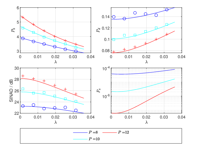
Fig. 4: Impact of the regularization parameter λ\lambda for different PP values. n=512n=512, δ=0.84\delta=0.84, ρ=2\rho=2 and σ=0.05\sigma=0.05. (Markers show the simulated results averaged over 50 realizations of random quantities 𝐇\mathbf{H}, 𝐬\mathbf{s} and 𝐳\mathbf{z}. We do not show simulated results for PeP_{e} because they require too many runs to simulate such a low PeP_{e}. )

By combining the observations in both regimes (ρ→0\rho\to 0 and OPENρ→∞)\rho\to\infty), we get a more precise idea of the role of the control parameter ρ\rho on the per-antenna power Pb⋆P_{b}^{\star}. Setting ρ\rho to small values makes the per-antenna power close to zero while using large values for ρ\rho leads the precoder to use the maximum allowed power at each antenna. Such behavior is illustrated in Figure 2, which plots Pb⋆P_{b}^{\star} against ρ\rho for several values of PP. As can be seen, by varying ρ\rho, the per-antenna power varies accordingly, becoming small for small ρ\rho values and close to the maximum allowed power for very large ρ\rho values. Note that, unlike RZF and ZF, the value of ρ\rho that achieves a fixed asymptotic per-antenna power Pb⋆P_{b}^{\star} can not be determined in an explicit form. In this respect, when it comes to comparing precoders, it is necessary to require the same Pb⋆P_{b}^{\star} value. This can be done for each precoder by using the value of ρ\rho that achieves the target Pb⋆P_{b}^{\star}. A plot like the one in Figure 2 can be used to determine numerically the corresponding values of the power control parameter.

By expanding ‖𝐇𝐱−ρ​𝐬‖2\|{\bf Hx}-\sqrt{\rho}{\bf s}\|^{2} in (72) and neglecting the quantities independent of ρ\rho or 𝐱{\bf x}, we may claim that for large ρ\rho values, the precoder in (72) would be close to the one bit-precoding 𝐱~:=P​sign​(𝐇T​𝐬)\tilde{\bf x}:=\sqrt{P}{\rm sign}({\bf H}^{T}{\bf s}). Such a finding, although making sense, calls into question the main interest behind solving the optimization problem in (2) to obtain the limited PAPR precoder. If for ρ→∞\rho\to\infty, its behavior would be equivalent to the precoder 𝐱~\tilde{\bf x} which uses the maximum allowed power, one can rightly think that it should be less complex and more efficient to use 𝐱~\tilde{\bf x} rather than solving the involved problem in (2). Such a conclusion would be correct if more power necessarily implies better performance. As evidenced later in the simulation section, it is possible for a precoder using a lower per-antenna power to perform better than the one-bit precoding scheme given by 𝐱~\tilde{\bf x} (See Figure 7 and Figure 8).

Numerical illustration. Figure 3 plots the theoretical values for all studied specifications and performance metrics against ρ\rho. In agreement with the results of Figure 2, the per-antenna power is an increasing function of ρ\rho, approaching PP when ρ\rho tends to infinity. However, when ρ\rho becomes very large, the distortion power increases, resulting in the saturation of the SINAD and the bit error probability. Interestingly, there is an optimal finite ρ\rho, and hence an optimal Pb⋆P_{b}^{\star} for which the performances in terms of SINAD and bit error probability are maximized.

IV Numerical simulations

In this section, we numerically investigate the performance of the limited PAPR precoders under different settings. We study the following specifications and performance metrics: the average per-user SINAD defined in (6), the average per-antenna power, the average per-user distortion power, and the bit error probability. We compare the results with the theoretical predictions derived in Section III. In all the figures below, solid lines represent the theoretical predictions, while markers show the simulated results averaged over 5050 realizations of random quantities 𝐇\mathbf{H}, 𝐬\mathbf{s} and 𝐳\mathbf{z}.

IV-A Impact of the regularization parameter λ\lambda

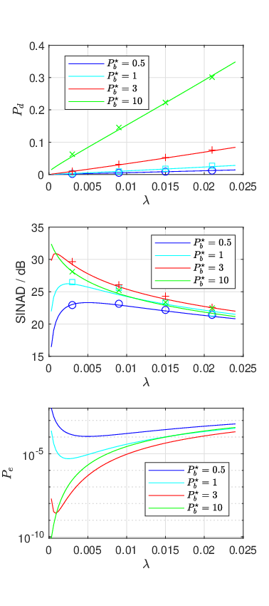
Figure 4 illustrates the behavior of various specifications and performance metrics with a varying regularization parameter for P=8,10P=8,10 and 1212. We note that the per-antenna power decreases with λ\lambda, since a large λ\lambda value would penalize the term ‖𝐱‖2\|{\bf x}\|^{2} in (2) more. However, as it can be seen from the plot of the bit error probability, setting λ\lambda to smaller values does not always translate into better performance. Indeed, a non-zero optimal value of λ\lambda exists, which is small for a large PP, but becomes larger as PP decreases. This shows that regularization is more important when PP is small to compensate for the bias caused by restricting the per-antenna power of the precoded vector. In a second experiment, we investigate whether this behavior still holds when all precoders have the same average per-antenna power. For that, we fix PP at 5050, and then use our asymptotic results to tune the power control factor ρ\rho to the value achieving the target Pb⋆P_{b}^{\star}. Figure 5 illustrates the obtained performances in terms of distortion power, the average per-user SINAD, and the bit error probability. Similar to Figure 4, we note that the optimal regularization parameter for low Pb⋆P_{b}^{\star} is larger than that for higher Pb⋆P_{b}^{\star}.

Refer to caption
Fig. 5: Impact of the regularization parameter λ\lambda for different Pb⋆P_{b}^{\star} values. P=50P=50, n=256n=256, δ=1\delta=1 and σ=0.05\sigma=0.05. Herein, the value of ρ\rho is tuned for each setting to achieve the target Pb⋆P_{b}^{\star}. We do not show simulated results for PeP_{e} because they require too many runs to simulate such a low PeP_{e}.

IV-B Impact of the number of users to the number of antennas ratio (δ\delta)

In Figure 6, we investigate the impact of the number of users to the number of antennas ratio δ\delta on the performance of the limited PAPR precoder. As in Figure 5, for each plot, we leverage our asymptotic analysis to set the power control parameter ρ\rho at the value ensuring the target asymptotic per-antenna power Pb⋆P_{b}^{\star}. As expected, we note that the power distortion increases with δ\delta. This is because a higher δ\delta translates into serving more users and thus causes higher distortion error levels. However, it is curious to note that the distortion error reaches very high levels as Pb⋆P_{b}^{\star} becomes of an order of magnitude of PP. To explain this, we refer to the findings of Theorem 8 and Figure 2, which suggest that a higher value of ρ\rho is required to reach higher values of Pb⋆P_{b}^{\star}. But, when ρ\rho is large, the distortion error automatically increases as it becomes difficult to approximate ρ​𝐬\sqrt{\rho}{\bf s} by 𝐇𝐱{\bf Hx} when 𝐱{\bf x} is constrained to a compact set. An important consequence of this behavior is that the SINAD performance and the bit error probability do not always improve by increasing the average per-antenna power Pb⋆P_{b}^{\star}. As shown in Figure 6, the performance is worse for Pb⋆=10P_{b}^{\star}=10 than for Pb⋆=3P_{b}^{\star}=3. This is because, for Pb⋆=10P_{b}^{\star}=10, the higher transmit power could not compensate for the higher distortion caused by using a higher value for ρ\rho.

Refer to caption
Fig. 6: Impact of δ\delta for different Pb⋆P_{b}^{\star} values. P=50P=50 n=256n=256, λ=0.002\lambda=0.002 and σ=0.05\sigma=0.05. The value of ρ\rho is tuned for each plot to achieve the target Pb⋆P_{b}^{\star}. We do not show simulated results for PeP_{e} because they require too many runs to simulate such a low PeP_{e}.
Refer to caption
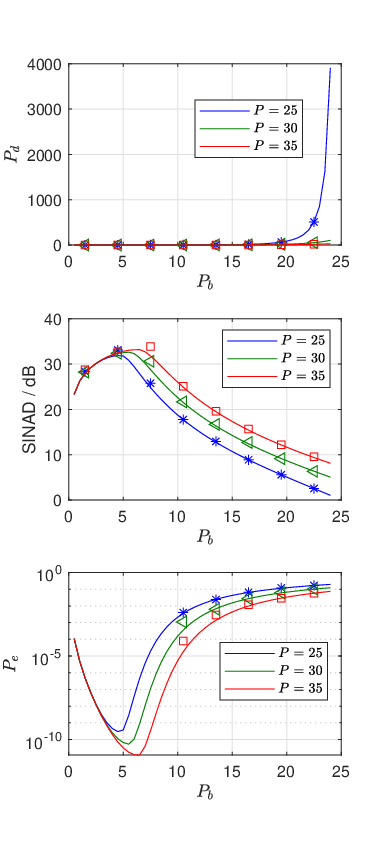
Fig. 7: The distortion power, SINAD and bit error probability versus PbP_{b}, for different PP values. n=256n=256, δ=1\delta=1 and σ=0.05\sigma=0.05. The control parameter ρ\rho is tuned to achieve the target Pb⋆P_{b}^{\star} and the regularization parameter λ\lambda is set to the value that maximizes the SINAD.

IV-C Comparison between precoders with optimal regularization

Figure 7 demonstrates the performance variation with PbP_{b} for P=25,30P=25,30, and 3535, when the regularization parameter λ\lambda is set to the value optimizing the SINAD. As in Figure 5 and Figure 6, ρ\rho is tuned to achieve the target Pb⋆P_{b}^{\star}. As an important remark, we note that there exists a Pb⋆P_{b}^{\star} for which the performances in terms of bit error probability and SINAD are optimal. This value is below PP. Indeed, as Pb⋆P_{b}^{\star} approaches PP, the distortion power significantly increases, resulting in a large performance deterioration. In a final experiment, we compare in Figure 8 the bit error probability performances of the limited PAPR precoder using optimal regularization with the one-bit precoding 𝐱~Pb=Pb⋆​sign​(𝐇T​𝐬)\tilde{\bf x}_{P_{b}}=\sqrt{P_{b}^{\star}}{\rm sign}({\bf H}^{T}{\bf s}). Complexitywise, the one-bit precoding possesses an explicit form and thus is more computationally efficient than the limited PAPR precoder which is based on solving a convex optimization problem. However, when it comes to bit error probability performance, we can easily see that the limited PAPR precoder is more efficient for all values of Pb⋆P_{b}^{\star}. As expected from Theorem 8, the performance gap is small when Pb⋆P_{b}^{\star} approaches PP but becomes much more pronounced when the limited PAPR precoder uses the optimal value of Pb⋆P_{b}^{\star}.

Refer to caption
Fig. 8: The bit error probability versus PbP_{b} given P=25P=25 (PbP_{b} increased by increasing the underlying ρ\rho ). Here we assign λ\lambda values which make optimal SINAD’s, n=256n=256, δ=1\delta=1 and σ=0.05\sigma=0.05.

V Conclusion

In this paper, we studied the asymptotic behavior of the limited PAPR precoder for multi-user communication systems in the regime in which the number of antennas and that of users grow large at the same pace. Contrary to the previous studies in [9] and [11], we rely on the CGMT framework and present approximations for other important performance metrics including the bit error probability and the average per user SINAD. To get more insights, we particularized our results to specific regimes in which the number of antennas is much larger than that of users, or the power control parameter takes very small or very high values. As a major outcome, our analysis demonstrates the existence of an optimal transmit power that maximizes the SINAD, and the bit error probability performances.

VI Proof of main results

VI-A The CGMT framework

In this section, we prove the main results in section III. The main technical ingredient is the CGMT. Before delving into the technical details of the proof, we provide a brief overview of the CGMT tool.

The CGMT is a mathematical framework that allows us to study the asymptotic behavior of high-dimensional optimization problems that can be written in the form of

Φ⁡(𝐆):=min𝐰∈𝒮𝐰​max𝐮∈𝒮𝐮​𝐮T​𝐆𝐰+ψ⁡(𝐰,𝐮),\Phi(\mathbf{G}):=\underset{\mathbf{w}\in\mathcal{S}_{\mathbf{w}}}{\min}\underset{\mathbf{u}\in\mathcal{S}_{\mathbf{u}}}{\max}\mathbf{u}^{T}\mathbf{Gw}+\psi(\mathbf{w},\mathbf{u}), (73)

where 𝐆∈ℝm×n\mathbf{G}\in\mathbb{R}^{m\times n} is a standard Gaussian matrix, ψ\psi is a real-valued function possibly random but independent of 𝐆{\bf G}, and 𝒮𝐰\mathcal{S}_{\bf w} and 𝒮𝐮\mathcal{S}_{\bf u} are two compact sets. The problem defined in (73) is known as the primary optimization problem (PO). The CGMT infers the behavior of the PO by considering the following associated auxiliary optimization problem (AO):

ϕ⁡(𝐠,𝐡):=min𝐰∈𝒮𝐰​max𝐮∈𝒮𝐮​‖𝐰‖​𝐠T​𝐮−|𝐮|𝐡T​𝐰+ψ⁡(𝐰,𝐮),\phi(\mathbf{g},\mathbf{h}):=\underset{\mathbf{w}\in\mathcal{S}_{\mathbf{w}}}{\min}\underset{\mathbf{u}\in\mathcal{S}_{\mathbf{u}}}{\max}\|\mathbf{w}\|\mathbf{g}^{T}\mathbf{u}-\|\mathbf{u}\|\mathbf{h}^{T}\mathbf{w}+\psi(\mathbf{w},\mathbf{u}), (74)

where 𝐠∈ℝm\mathbf{g}\in\mathbb{R}^{m} and 𝐡∈ℝn\mathbf{h}\in\mathbb{R}^{n} two standard Gaussian vectors. More formally the CGMT is stated as follows:

Theorem 9 (CGMT).

Consider the optimization problems in (73) and (74) The following statements hold true:

  • •

    For all t∈ℝt\in\mathbb{R},

    ℙ[Φ(𝐆)≤t]≤2ℙ[ϕ(𝐠,𝐡)≤t].\mathbb{P}\left[\Phi(\mathbf{G})\leq t\right]\leq 2\mathbb{P}\left[\phi({\bf g},{\bf h})\leq t\right]. (75)
  • •

    If additionally 𝒮𝐰\mathcal{S}_{\bf w} and 𝒮𝐮\mathcal{S}_{\bf u} are convex and ψ\psi is convex-concave, then for all t∈ℝt\in\mathbb{R},

    ℙ[Φ(𝐆)≥t]≤2ℙ[ϕ(𝐠,𝐡)≥t].\mathbb{P}\left[\Phi(\mathbf{G})\geq t\right]\leq 2\mathbb{P}\left[\phi({\bf g},{\bf h})\geq t\right]. (76)

    Particularly, for any ν≥0\nu\geq 0 it holds that:

    ℙ[|Φ(𝐆)−ν|≥t]≤2ℙ[|ϕ(𝐠,𝐡)−ν|≥t].\mathbb{P}\left[\left|\Phi(\mathbf{G})-\nu\right|\geq t\right]\leq 2\mathbb{P}\left[\left|\phi({\bf g},{\bf h})-\nu\right|\geq t\right].

According to the first statement in Theorem 9,

ℙ[Φ(𝐆)≤t]≤2ℙ[ϕ(𝐠,𝐡)≤t].\mathbb{P}\left[\Phi(\mathbf{G})\leq t\right]\leq 2\mathbb{P}\left[\phi({\bf g},{\bf h})\leq t\right].

Equivalently stated, this implies that a high-probability lower bound of the AO cost is also a high probability lower bound of the PO. Such a result holds even when the sets or the function ψ\psi are not convex.

However, the main interest in the CGMT lies in the second statement of Theorem 9, which affirms that under convexity conditions of the PO, the AO can be used to infer properties on the PO’s asymptotic cost. More precisely, if for some ν\nu, the AO cost concentrates around ν\nu, so does cost of the PO. Moreover, as shall be shown next, under appropriate strong-convexity conditions with respect to the solutions of the AO, the CGMT shows that concentration of Lipschitz functions of the solution of the AO implies concentration of that of the PO.

In the sequel, we make use of the CGMT framework to analyze the performance of the PAPR precoding scheme. As a first step, we express the PAPR precoding problem as a PO problem.

VI-B Relating the PAPR precoding problem to POs

Formulation of the POs. For 𝕏=[−P,P]\mathbb{X}=[-\sqrt{P},\sqrt{P}], the solution of the regularized least squares problem is given by

𝐱^=arg⁡minxi2≤P​1n​‖𝐇𝐱−ρ​𝐬‖2+λn​‖𝐱‖2,\hat{\bf x}=\arg\min_{x_{i}^{2}\leq P}\frac{1}{n}\|{\bf Hx}-\sqrt{\rho}{\bf s}\|^{2}+\frac{\lambda}{n}\|{\bf x}\|^{2}, (77)

where compared to (2), we normalized the optimization cost by 1n\frac{1}{n}. Using the following identity:

‖𝐳‖2=max𝐮∈ℝm⁡𝐮T​𝐳−‖𝐮‖24,\|{\bf z}\|^{2}=\max_{{\bf u}\in\mathbb{R}^{m}}{\bf u}^{T}{\bf z}-\frac{\|{\bf u}\|^{2}}{4},

which holds for any vector 𝐳∈ℝm{\bf z}\in\mathbb{R}^{m}, we can write the optimization problem in (77) as

minxi2≤P​max𝐮​n​𝐮T​𝐇𝐱n−ρ​𝐮T​𝐬n−‖𝐮‖24+λ​‖𝐱‖2n.\underset{x_{i}^{2}\leq P}{\min}\underset{\mathbf{u}}{\max}\frac{\sqrt{n}\mathbf{u}^{T}\mathbf{Hx}}{n}-\frac{\sqrt{\rho}\mathbf{u}^{T}\mathbf{s}}{\sqrt{n}}-\frac{\|\mathbf{u}\|^{2}}{4}+\frac{\lambda\|\mathbf{x}\|^{2}}{n}. (78)

The above problem is in the form of the PO, except that the constraint set over 𝐮{\bf u} is not bounded. From first-order optimality conditions, we can easily check that the optimal 𝐮{\bf u} is given by

𝐮⋆=2​(1n​𝐇𝐱−ρ​𝐬n).{\bf u}^{\star}=2\left(\frac{1}{\sqrt{n}}{\bf Hx}-\frac{\sqrt{\rho}{\bf s}}{\sqrt{n}}\right).

Hence,

‖𝐮⋆‖≤2​P​‖𝐇‖+ρ​mn.\|{\bf u}^{\star}\|\leq 2\sqrt{P}\left\|{\bf H}\right\|+\frac{\sqrt{\rho}\sqrt{m}}{\sqrt{n}}.

Also, using standard inequalities of the spectral norm of Gaussian matrices, we can prove that ‖𝐇‖≤ℬ\|{\bf H}\|\leq\mathcal{B} with probability approaching 11 for some positive constant ℬ\mathcal{B}. All this shows that ‖𝐮⋆‖\|{\bf u}^{\star}\| is bounded with probability approaching 11. Thus the analysis would not thus change if we instead consider the following problem:

minxi2≤P​max𝐮∈𝒮𝐮​n​𝐮T​𝐇𝐱n−ρ​𝐮T​𝐬n−‖𝐮‖24+λ​‖𝐱‖2n,\underset{x_{i}^{2}\leq P}{\min}\underset{\mathbf{u}\in\mathcal{S}_{\mathbf{u}}}{\max}\frac{\sqrt{n}\mathbf{u}^{T}\mathbf{Hx}}{n}-\frac{\sqrt{\rho}\mathbf{u}^{T}\mathbf{s}}{\sqrt{n}}-\frac{\|\mathbf{u}\|^{2}}{4}+\frac{\lambda\|\mathbf{x}\|^{2}}{n}, (79)

where 𝒮𝐮={𝐮∈ℝm,∥𝐮∥≤ℬ}\mathcal{S}_{\bf u}=\left\{{\bf u}\in\mathbb{R}^{m},\ \ \|{\bf u}\|\leq\mathcal{B}\right\} for some ℬ>0\mathcal{B}>0 is a high-probability upper bound on 2​‖𝐮⋆‖2\|{\bf u}^{\star}\|. Our interest is to characterize the asymptotic behavior of the solutions in 𝐱{\bf x} and 𝐮{\bf u} to (79), which perfectly agrees with the conditions required by the CGMT. For that, we introduce the following cost functions:

𝒞λ,ρ​(𝐱)=max𝐮∈𝒮𝐮⁡n​𝐮T​𝐇𝐱n−ρ​𝐮T​𝐬n−‖𝐮‖24+λ​‖𝐱‖2n,\displaystyle\mathcal{C}_{\lambda,\rho}({\bf x})=\max_{{\bf u}\in\mathcal{S}_{{\bf u}}}\frac{\sqrt{n}{\bf u}^{T}{\bf Hx}}{n}-\frac{\sqrt{\rho}{\bf u}^{T}{\bf s}}{\sqrt{n}}-\frac{\|{\bf u}\|^{2}}{4}+\frac{\lambda\|{\bf x}\|^{2}}{n}, (80)
𝒱λ,ρ​(𝐮)=minxi2≤P⁡n​𝐮T​𝐇𝐱n−ρ​𝐮T​𝐬n−‖𝐮‖24+λ​‖𝐱‖2n,\displaystyle\mathcal{V}_{\lambda,\rho}({\bf u})=\min_{x_{i}^{2}\leq P}\frac{\sqrt{n}{\bf u}^{T}{\bf Hx}}{n}-\frac{\sqrt{\rho}{\bf u}^{T}{\bf s}}{\sqrt{n}}-\frac{\|{\bf u}\|^{2}}{4}+\frac{\lambda\|{\bf x}\|^{2}}{n}, (81)

and consider the following primary problems:

Φλ,ρ​(𝐇)\displaystyle\Phi_{\lambda,\rho}({\bf H}) :=minxi2≤P⁡𝒞λ,ρ​(𝐱),\displaystyle:=\min_{x_{i}^{2}\leq P}\mathcal{C}_{\lambda,\rho}({\bf x}), (82)
Φ~λ,ρ​(𝐇)\displaystyle\tilde{\Phi}_{\lambda,\rho}({\bf H}) :=max𝐮∈𝒮𝐮⁡𝒱λ,ρ​(𝐮).\displaystyle:=\max_{{\bf u}\in\mathcal{S}_{\bf u}}\mathcal{V}_{\lambda,\rho}({\bf u}). (83)

Since the objective function in (79) is convex in 𝐱{\bf x} and concave in 𝐮{\bf u}, then

Φλ,ρ​(𝐇)=Φ~λ,ρ​(𝐇),\Phi_{\lambda,\rho}({\bf H})=\tilde{\Phi}_{\lambda,\rho}({\bf H}), (84)

and the solutions 𝐱^PO\hat{\bf x}_{\rm PO} and 𝐮^PO\hat{\bf u}_{\rm PO} to (79) are given by 22 2 Note that the objective in (79) is strictly convex in 𝐱{\bf x} and strictly concave in 𝐮{\bf u}. Hence, the solutions 𝐱{\bf x} and 𝐮{\bf u} are unique.:

𝐱^PO:=arg⁡minxi2≤P​𝒞λ,ρ​(𝐱),\displaystyle\hat{\bf x}_{\rm PO}:=\arg\min_{x_{i}^{2}\leq P}\mathcal{C}_{\lambda,\rho}({\bf x}), (85)
𝐮^PO:=arg⁡max𝐮∈𝒮𝐮​𝒱λ,ρ​(𝐮).\displaystyle\hat{\bf u}_{\rm PO}:=\arg\max_{{\bf u}\in\mathcal{S}_{\bf u}}\mathcal{V}_{\lambda,\rho}({\bf u}). (86)

Formulation of the AOs. With the PO problems in (82) and (83), we associate the following AO problems:

ϕλ,ρ​(𝐠,𝐡)\displaystyle\phi_{\lambda,\rho}({\bf g},{\bf h}) :=minxi2≤P⁡ℒλ,ρ​(𝐱),\displaystyle:=\min_{x_{i}^{2}\leq P}\mathcal{L}_{\lambda,\rho}({\bf x}), (87)
ϕ~λ,ρ​(𝐠,𝐡)\displaystyle\tilde{\phi}_{\lambda,\rho}({\bf g},{\bf h}) =max𝐮∈𝒮𝐮⁡ℱλ,ρ​(𝐮),\displaystyle=\max_{{\bf u}\in\mathcal{S}_{{\bf u}}}\mathcal{F}_{\lambda,\rho}({\bf u}), (88)

where ℒλ,ρ​(𝐱)\mathcal{L}_{\lambda,\rho}({\bf x}) and ℱλ,ρ​(𝐮)\mathcal{F}_{\lambda,\rho}({\bf u}) are given by

ℒλ,ρ​(𝐱):=max𝐮∈𝒮𝐮​1n​‖𝐱‖​𝐠T​𝐮−1n​‖𝐮‖​𝐡T​𝐱−ρ​𝐮T​𝐬n−‖𝐮‖24+λ​‖𝐱‖2n,\displaystyle\mathcal{L}_{\lambda,\rho}({\bf x}):=\underset{\mathbf{u}\in\mathcal{S}_{\mathbf{u}}}{\max}\frac{1}{n}\|\mathbf{x}\|\mathbf{g}^{T}\mathbf{u}-\frac{1}{n}\|\mathbf{u}\|\mathbf{h}^{T}\mathbf{x}-\frac{\sqrt{\rho}\mathbf{u}^{T}\mathbf{s}}{\sqrt{n}}-\frac{\|\mathbf{u}\|^{2}}{4}+\frac{\lambda\|\mathbf{x}\|^{2}}{n}, (89)
ℱλ,ρ​(𝐮):=minxi2≤P⁡1n​‖𝐱‖​𝐠T​𝐮−1n|𝐮|𝐡T​𝐱−ρ​𝐮T​𝐬n−‖𝐮‖24+λ​‖𝐱‖2n.\displaystyle\mathcal{F}_{\lambda,\rho}({\bf u}):=\min_{x_{i}^{2}\leq P}\frac{1}{n}\|\mathbf{x}\|\mathbf{g}^{T}\mathbf{u}-\frac{1}{n}\|\mathbf{u}\|\mathbf{h}^{T}\mathbf{x}-\frac{\sqrt{\rho}\mathbf{u}^{T}\mathbf{s}}{\sqrt{n}}-\frac{\|\mathbf{u}\|^{2}}{4}+\frac{\lambda\|\mathbf{x}\|^{2}}{n}. (90)

Similarly, we define the solutions 𝐱^AO\hat{\bf x}^{\rm AO} and 𝐮^AO\hat{\bf u}^{\rm AO} as

𝐱^AO\displaystyle\hat{\bf x}^{\rm AO} :=arg⁡min𝐱xi2≤P​ℒλ,ρ​(𝐱),\displaystyle:=\arg\min_{\begin{subarray}{c}{\bf x}\\ x_{i}^{2}\leq P\end{subarray}}\mathcal{L}_{\lambda,\rho}({\bf x}), (91)
𝐮^AO\displaystyle\hat{\bf u}^{\rm AO} :=arg⁡max𝐮∈𝒮𝐮​ℱλ,ρ​(𝐮).\displaystyle:=\arg\max_{{\bf u}\in\mathcal{S}_{\mathbf{u}}}\mathcal{F}_{\lambda,\rho}({\bf u}). (92)

The objective of the CGMT is to prove that the properties of the solutions of the PO defined in (85) and (86) can be transferred to the solutions of the AO defined in (91) and (92). This can be performed by using the following inequalities which directly follow as a direct application of Theorem 9.

  • •

    For all t∈ℝt\in\mathbb{R} and any compact sets 𝒮~𝐱\tilde{\mathcal{S}}_{{\bf x}} and 𝒮~𝐮\tilde{\mathcal{S}}_{\bf u},

    ℙ[min𝐱∈𝒮~𝐱𝒞λ,ρ(𝐱)≤t]≤2ℙ[min𝐱∈𝒮~𝐱ℒλ,ρ(𝐱)≤t],\displaystyle\mathbb{P}\left[\min_{{\bf x}\in\tilde{\mathcal{S}}_{{\bf x}}}\mathcal{C}_{\lambda,\rho}({\bf x})\leq t\right]\leq 2\mathbb{P}\left[\min_{{\bf x}\in\tilde{\mathcal{S}}_{{\bf x}}}\mathcal{L}_{\lambda,\rho}({\bf x})\leq t\right], (93)
    ℙ[max𝐮∈𝒮~𝐮𝒱λ,ρ(𝐮)≥t]≤2ℙ[max𝐮∈𝒮~𝐮ℱλ,ρ(𝐮)≥t].\displaystyle\mathbb{P}\left[\max_{{\bf u}\in\tilde{\mathcal{S}}_{{\bf u}}}\mathcal{V}_{\lambda,\rho}({\bf u})\geq t\right]\leq 2\mathbb{P}\left[\max_{{\bf u}\in\tilde{\mathcal{S}}_{{\bf u}}}\mathcal{F}_{\lambda,\rho}({\bf u})\geq t\right]. (94)
  • •

    If the sets 𝒮𝐱\mathcal{S}_{{\bf x}} and 𝒮𝐮\mathcal{S}_{\bf u} are convex, we have for all t∈ℝt\in\mathbb{R},

    ℙ[min𝐱∈𝒮𝐱𝒞λ,ρ(𝐱)≥t]≤2ℙ[min𝐱∈𝒮𝐱ℒλ,ρ(𝐱)≥t],\displaystyle\mathbb{P}\left[\min_{{\bf x}\in\mathcal{S}_{{\bf x}}}\mathcal{C}_{\lambda,\rho}({\bf x})\geq t\right]\leq 2\mathbb{P}\left[\min_{{\bf x}\in\mathcal{S}_{{\bf x}}}\mathcal{L}_{\lambda,\rho}({\bf x})\geq t\right], (95)
    ℙ[max𝐮∈𝒮𝐮𝒱λ,ρ(𝐮)≤t]≤2ℙ[max𝐮∈𝒮𝐮ℱλ,ρ(𝐮)≤t].\displaystyle\mathbb{P}\left[\max_{{\bf u}\in\mathcal{S}_{{\bf u}}}\mathcal{V}_{\lambda,\rho}({\bf u})\leq t\right]\leq 2\mathbb{P}\left[\max_{{\bf u}\in\mathcal{S}_{{\bf u}}}\mathcal{F}_{\lambda,\rho}({\bf u})\leq t\right]. (96)

Particularly, the above inequalities can be used to prove concentrations of the optimal cost of the PO. Interestingly, they can also lead to transfer concentrations of the optimal solution of the AO to that of the PO, under some strong-convexity properties on the AO problem. It is thus a key step before delving into the technical proofs of Theorem 1 and Theorem 2 to analyze the behavior of the AO problems in (87) and (88). This is the main purpose of the following Lemmas, the proof of which is deferred to Section VII and VIII to avoid disrupting the flow of the proof. Particularly, Lemma 1 establishes the uniqueness and the existence of the solutions to the asymptotic AO problem introduced in Theorem 1. Lemma 2 and Lemma 3 provide the technical ingredients to study the asymptotic behavior of the solutions 𝐱^AO\hat{\bf x}^{\rm AO} and 𝐮^AO\hat{\bf u}^{\rm AO} in (91) and (92).

Lemma 1 (Behavior of the asymptotic optimization problem).

Define ϕ¯\overline{\phi} as the following deterministic max-min problem:

ϕ¯:=maxβ≥0⁡minτ≥0𝒟⁡(β,τ):=τ​β​δ2+ρ​β2​τ−β24+Y⁡(β,τ),\overline{\phi}:=\max_{\beta\geq 0}\min_{\tau\geq 0}\ \ \mathcal{D}(\beta,\tau):=\frac{\tau\beta\delta}{2}+\frac{\rho\beta}{2\tau}-\frac{\beta^{2}}{4}+Y(\beta,\tau), (97)

where Y⁡(β,τ)Y(\beta,\tau) is given by

Y⁡(β,τ)\displaystyle Y(\beta,\tau) :=βP𝔼[(Pα−2H)𝟏{H≥Pα}]−β2​α𝔼[H2𝟏{−Pα≤H≤Pα}]\displaystyle:=\beta\sqrt{P}\mathbb{E}\left[\left(\sqrt{P}\alpha-2H\right){\bf 1}_{\{H\geq\sqrt{P}\alpha\}}\right]-\frac{\beta}{2\alpha}\mathbb{E}\left[H^{2}{\bf 1}_{\{-\sqrt{P}\alpha\leq H\leq\sqrt{P}\alpha\}}\right] (98)
=βα(𝔼[(H−Pα)2𝟏{H≥Pα}]−12)\displaystyle=\frac{\beta}{\alpha}\left(\mathbb{E}\left[(H-\sqrt{P}\alpha)^{2}{\bf 1}_{\{H\geq\sqrt{P}\alpha\}}\right]-\frac{1}{2}\right) (99)

and 33 3 The compact expression in (99) is easily obtained by noticing that 𝔼[H2𝟏{−Pα≤H≤Pα}]=1−2𝔼[H2𝟏{H≥Pα}]\mathbb{E}\left[H^{2}{\bf 1}_{\{-\sqrt{P}\alpha\leq H\leq\sqrt{P}\alpha\}}\right]=1-2\mathbb{E}\left[H^{2}{\bf 1}_{\{H\geq\sqrt{P}\alpha\}}\right]. α=1/τ+2​λ/β\alpha=1/\tau+2\lambda/\beta . Then the following statements hold:

  1. 1.

    The function β↦𝒟⁡(β,τ)\beta\mapsto\mathcal{D}(\beta,\tau) is strictly concave.

  2. 2.

    The above optimization problem possesses a unique finite saddle point (β⋆,τ⋆)(\beta^{\star},\tau^{\star}) if and only if λ>0\lambda>0 or λ=0\lambda=0 and δ>1\delta>1. Moreover, in both cases β⋆>0\beta^{\star}>0.

  3. 3.

    The solution τ⋆\tau^{\star} satisfies the following equation:

    (τ⋆)2​δ−ρ\displaystyle(\tau^{\star})^{2}\delta-\rho =2Pℙ[H≥Pα⋆]+1(α⋆)2𝔼[H2𝟏{−Pα⋆≤H≤Pα⋆}].\displaystyle=2P\mathbb{P}\left[H\geq\sqrt{P}\alpha^{\star}\right]+\frac{1}{(\alpha^{\star})^{2}}\mathbb{E}\left[H^{2}{\bf 1}_{\{-\sqrt{P}\alpha^{\star}\leq H\leq\sqrt{P}\alpha^{\star}\}}\right]. (100)
  4. 4.

    Assume λ=0\lambda=0 and δ>1\delta>1. Then the saddle point (β⋆,τ⋆)(\beta^{\star},\tau^{\star}) of (97) is given by:

    τ⋆\displaystyle\tau^{\star} =arg⁡minτ≥0⁡(τ​δ2+ρ2​τ+Y~​(τ))+2,\displaystyle=\arg\min_{\tau\geq 0}\left(\frac{\tau\delta}{2}+\frac{\rho}{2\tau}+\tilde{Y}(\tau)\right)_{+}^{2}, (101)
    β⋆\displaystyle\beta^{\star} =(τ⋆​δ+ρτ⋆+2​Y~​(τ⋆))+,\displaystyle=\left({\tau^{\star}\delta}+\frac{\rho}{\tau^{\star}}+2\tilde{Y}(\tau^{\star})\right)_{+}, (102)

    and (97) reduces to:

    ϕ¯:=minτ≥0⁡(τ​δ2+ρ2​τ+Y~​(τ))+2.\overline{\phi}:=\min_{\tau\geq 0}\left(\frac{\tau\delta}{2}+\frac{\rho}{2\tau}+\tilde{Y}(\tau)\right)_{+}^{2}.

    where

    Y~​(τ)\displaystyle\tilde{Y}(\tau) =P𝔼[(Pτ−2H)𝟏{H≥Pτ}]−τ2𝔼[H2𝟏{−Pτ≤H≤Pτ}]\displaystyle=\sqrt{P}\mathbb{E}\left[\left(\frac{\sqrt{P}}{\tau}-2H\right){\bf 1}_{\{H\geq\frac{\sqrt{P}}{\tau}\}}\right]-\frac{\tau}{2}\mathbb{E}\left[H^{2}{\bf 1}_{\{-\frac{\sqrt{P}}{\tau}\leq H\leq\frac{\sqrt{P}}{\tau}\}}\right] (103)
    =τ(𝔼[(H−Pτ)2𝟏{H≥Pτ}]−12).\displaystyle=\tau\left(\mathbb{E}\left[(H-\frac{\sqrt{P}}{\tau})^{2}{\bf 1}_{\{H\geq\frac{\sqrt{P}}{\tau}\}}\right]-\frac{1}{2}\right). (104)

    Moreover, τ⋆\tau^{\star} is the unique solution to the following equation:

    τ2δ−ρ=2Pℙ[H≥Pτ]+τ2𝔼[H2𝟏{−Pτ≤H≤Pτ}].\tau^{2}\delta-\rho=2P\mathbb{P}\left[H\geq\frac{\sqrt{P}}{\tau}\right]+\tau^{2}\mathbb{E}\left[H^{2}{\bf 1}_{\{-\frac{\sqrt{P}}{\tau}\leq H\leq\frac{\sqrt{P}}{\tau}\}}\right]. (105)
Proof.

See Section VII. ∎

Lemma 2.

Let ϕ¯\overline{\phi} be the deterministic max-min problem defined in (97), and denote by (β⋆,τ⋆)(\beta^{\star},\tau^{\star}) its associated saddle point. Define 𝐱¯AO\overline{\bf x}^{\rm AO} as follows:

[𝐱¯AO]i:={−P,hi≤−P​α⋆hiα⋆,−P​α⋆≤hi≤P​α⋆P,hi≥P​α⋆,\left[\overline{\bf x}_{\rm AO}\right]_{i}:=\left\{\begin{array}[]{ll}-\sqrt{P},&h_{i}\leq-\sqrt{P}\alpha^{\star}\\ \frac{h_{i}}{\alpha^{\star}},&-\sqrt{P}\alpha^{\star}\leq h_{i}\leq\sqrt{P}\alpha^{\star}\\ \sqrt{P},&h_{i}\geq\sqrt{P}\alpha^{\star}\end{array},\right.

where α⋆=1/τ⋆+2​λ/β⋆\alpha^{\star}=1/\tau^{\star}+2\lambda/\beta^{\star} , hih_{i}’s are independent standard Gaussian random variables. Then, the following statements hold true:

  1. 1.

    There exists a function ℒ^λ,ρ​(𝐱)\hat{\mathcal{L}}_{\lambda,\rho}({\bf x}) such that

    • •

      The function 𝐱↦ℒ^λ,ρ​(𝐱){\bf x}\mapsto\hat{\mathcal{L}}_{\lambda,\rho}({\bf x}) is λn\frac{\lambda}{n}-strongly convex for λ>0\lambda>0 and locally strongly convex in a neighborhood of 𝐱¯AO\overline{\bf x}^{\rm AO} when λ=0\lambda=0 and δ>1\delta>1.

    • •

      The following convergences holds true:

      sup𝐱xi2≤P|ℒ^λ,ρ​(𝐱)−ℒλ,ρ​(𝐱)|→P0,\sup_{\begin{subarray}{c}{\bf x}\\ x_{i}^{2}\leq P\end{subarray}}\left|\hat{\mathcal{L}}_{\lambda,\rho}({\bf x})-\mathcal{L}_{\lambda,\rho}({\bf x})\right|\stackrel{{\scriptstyle P}}{{\rightarrow}}0,

      and

      min𝐱xi2≤P⁡ℒ^λ,ρ​(𝐱)−ϕ¯→P0.\min_{\begin{subarray}{c}{\bf x}\\ x_{i}^{2}\leq P\end{subarray}}\hat{\mathcal{L}}_{\lambda,\rho}({\bf x})-\overline{\phi}\stackrel{{\scriptstyle P}}{{\rightarrow}}0.
  2. 2.

    Let 𝐱~AO\tilde{\bf x}^{\rm AO} be a minimizer of ℒ^λ,ρ\hat{\mathcal{L}}_{\lambda,\rho}. Then, for any ϵ>0\epsilon>0, with probability approaching 11,

    1n​‖𝐱~AO−𝐱¯AO‖≤ϵ,\frac{1}{n}\|\tilde{\bf x}^{\rm AO}-\overline{\bf x}^{\rm AO}\|\leq\epsilon,

    and

    ℒ^λ,ρ​(𝐱¯AO)≤min𝐱𝐱𝐢𝟐≤𝐏⁡ℒ^λ,ρ​(𝐱)+ϵ.\hat{\mathcal{L}}_{\lambda,\rho}(\overline{\bf x}^{\rm AO})\leq\min_{\begin{subarray}{c}{\bf x}\\ x_{i}^{2}\leq P\end{subarray}}\hat{\mathcal{L}}_{\lambda,\rho}({\bf x})+\epsilon. (106)
Proof.

See Section VIII-A. ∎

Lemma 3.

Consider the setting of Lemma 2. Then, the following statements hold true:

  1. 1.

    With probability approaching 11, we have

    |ϕ~λ,ρ​(𝐠,𝐡)−ϕ¯|→P0.\left|\tilde{\phi}_{\lambda,\rho}({\bf g},{\bf h})-\overline{\phi}\right|\stackrel{{\scriptstyle P}}{{\rightarrow}}0. (107)
  2. 2.

    Define ℱ~λ,ρ​(𝐮)\tilde{\mathcal{F}}_{\lambda,\rho}({\bf u}) as

    ℱ~λ,ρ​(𝐮)\displaystyle\tilde{\mathcal{F}}_{\lambda,\rho}({\bf u}) =1n​‖𝐱¯AO‖​𝐠𝐓​𝐮−𝟏𝐧​‖𝐮‖​𝐡𝐓​𝐱¯AO−ρ𝐧​𝐮𝐓​𝐬−‖𝐮‖𝟐𝟒+λ𝐧​‖𝐱¯AO‖𝟐,\displaystyle=\frac{1}{n}\|\overline{\bf x}^{\rm AO}\|{\bf g}^{T}{\bf u}-\frac{1}{n}\|{\bf u}\|{\bf h}^{T}\overline{\bf x}^{\rm AO}-\frac{\sqrt{\rho}}{\sqrt{n}}{\bf u}^{T}{\bf s}-\frac{\|{\bf u}\|^{2}}{4}+\frac{\lambda}{n}\|\overline{\bf x}^{\rm AO}\|^{2}, (108)

    then ℱ~λ,ρ\tilde{\mathcal{F}}_{\lambda,\rho} is 12\frac{1}{2}-strongly-concave, and

    |max𝐮⁡ℱ~λ,ρ​(𝐮)−ϕ¯|→P0.\left|\max_{{\bf u}}\mathcal{\tilde{F}}_{\lambda,\rho}({\bf u})-\overline{\phi}\right|\stackrel{{\scriptstyle P}}{{\rightarrow}}0. (109)
  3. 3.

    Denote by 𝐮~AO\tilde{\bf u}^{\rm AO} the maximizer of ℱ~λ,ρ\tilde{\mathcal{F}}_{\lambda,\rho}:

    𝐮~AO=arg⁡max𝐮​ℱ~λ,ρ​(𝐮),\tilde{\bf u}^{\rm AO}=\arg\max_{{\bf u}}\tilde{\mathcal{F}}_{\lambda,\rho}({\bf u}),

    let 𝐮¯AO\overline{\bf u}^{\rm AO} be given by

    𝐮¯AO=β⋆​((τ⋆)𝟐​δ−ρ​𝐠−ρ​𝐬)τ⋆​δ​𝐧,\overline{\bf u}^{\rm AO}=\frac{\beta^{\star}(\sqrt{(\tau_{\star})^{2}\delta-\rho}{\bf g}-\sqrt{\rho}{\bf s})}{\tau^{\star}\delta\sqrt{n}},

    then for any ϵ>0\epsilon>0, with probability approaching 11,

    ‖𝐮¯AO−𝐮~AO‖≤ϵ.\|\overline{\bf u}^{\rm AO}-\tilde{\bf u}^{\rm AO}\|\leq\epsilon. (110)
Proof.

See Section VIII-B. ∎

VI-C Proof of Theorem 1

With Lemma 2 at hand, we are now ready to develop Theorem 1. Let ff be a Lipschitz function. For 𝐱∈ℝn{\bf x}\in\mathbb{R}^{n} we define

F⁡(𝐱)=1n​∑i=1nf⁡(𝐱i)F({\bf x})=\frac{1}{n}\sum_{i=1}^{n}f({\bf x}_{i})

and κ=𝔼H​[f⁡(θ⁡(H))]\kappa=\mathbb{E}_{H}\left[f(\theta(H))\right]. For any ϵ>0\epsilon>0, define the set

𝒮={𝐱∈ℝn,xi2≤P||F(𝐱)−κ|≥2ϵ}.\mathcal{S}=\left\{{\bf x}\in\mathbb{R}^{n},x_{i}^{2}\leq P|\left|F({\bf x})-\kappa\right|\geq 2\epsilon\right\}.

Consider the following ’perturbed’ PO and AO problems

Φ𝒮​(𝐇)=min𝐱∈𝒮⁡𝒞λ,ρ​(𝐱),\Phi_{\mathcal{S}}({\bf H})=\min_{{\bf x}\in\mathcal{S}}\mathcal{C}_{\lambda,\rho}({\bf x}),

and

ϕ𝒮​(𝐠,𝐡)=min𝐱∈𝒮⁡ℒλ,ρ​(𝐱).\phi_{\mathcal{S}}({\bf g},{\bf h})=\min_{{\bf x}\in\mathcal{S}}\mathcal{L}_{\lambda,\rho}({\bf x}).

To prove the third statement of Theorem 1, it suffices to show that with probability approaching 11,

ΦS​(𝐇)>Φλ,ρ​(𝐇).\Phi_{S}({\bf H})>\Phi_{\lambda,\rho}({\bf H}). (111)

Using the CGMT, and as shown in [15], it suffices to find constants ϕ¯S\overline{\phi}_{S} and η\eta such that with probability approaching 11, the following statements hold true:

  1. 1.

    ϕ¯S≥ϕ¯+3​η\overline{\phi}_{S}\geq\overline{\phi}+3\eta,

  2. 2.

    ϕλ,ρ​(𝐠,𝐡)≤ϕ¯+η{\phi}_{\lambda,\rho}({\bf g},{\bf h})\leq\overline{\phi}+\eta,

  3. 3.

    ϕ𝒮​(𝐠,𝐡)≥ϕ¯S−η\phi_{\mathcal{S}}({\bf g},{\bf h})\geq\overline{\phi}_{S}-\eta.

Indeed, if the three statements above are satisfied, then from (93),

ℙ[ΦS(𝐇)≤ϕ¯S−η]≤2ℙ[ϕS(𝐠,𝐡)≤ϕ¯S−η],\mathbb{P}\left[\Phi_{S}({\bf H})\leq\overline{\phi}_{S}-\eta\right]\leq 2\mathbb{P}\left[\phi_{S}({\bf g},{\bf h})\leq\overline{\phi}_{S}-\eta\right],

while from statement OPEN3)3)

ℙ[ϕS(𝐠,𝐡)≤ϕ¯S−η]→0.\mathbb{P}\left[\phi_{S}({\bf g},{\bf h})\leq\overline{\phi}_{S}-\eta\right]\to 0.

Hence, with probability approaching 11,

ΦS​(𝐇)≥ϕ¯S−η,\Phi_{S}({\bf H})\geq\overline{\phi}_{S}-\eta,

and thus, from Statement OPEN1)1),

ΦS​(𝐇)≥ϕ¯+2​η.\Phi_{S}({\bf H})\geq\overline{\phi}+2\eta. (112)

On the other hand, we can in a similar way use (95) together with Statement OPEN2)2), to show that with probability approaching 11,

Φλ,ρ​(𝐇)≤ϕ¯+η.\Phi_{\lambda,\rho}({\bf H})\leq\overline{\phi}+\eta. (113)

Combining (112) with (113) yields the desired relation in (111).

In the remaining, we consider finding ϕ¯S\overline{\phi}_{S} and η\eta values for which the aforementioned statements hold.

Proof of Statement OPEN2)2). From Lemma 2, it holds that with probability approaching 1,

ϕλ,ρ​(𝐠,𝐡)≤ϕ¯+η,\phi_{\lambda,\rho}({\bf g},{\bf h})\leq\overline{\phi}+\eta,

which shows that Statement OPEN2)2) holds for any η>0\eta>0.

Proof of Statement OPEN3)3). As a first step, we show that Statement OPEN3)3) holds if for an appropriate choice of ϵ~\tilde{\epsilon}, it holds that

∀𝐱∈𝒮,a8​n​‖𝐱−𝐱¯AO‖2≥ϵ~.\forall{\bf x}\in\mathcal{S},\ \ \frac{a}{8n}\left\|{\bf x}-\overline{\bf x}^{\rm AO}\right\|^{2}\geq\tilde{\epsilon}. (114)

To see this, recall that from Lemma 2, the function ℒ^\hat{\mathcal{L}} is an\frac{a}{n}-strongly convex in a neighborhood of 𝐱¯AO\overline{\bf x}^{\rm AO}. Moreover, for some ϵ\epsilon sufficiently small, we have proved in (106) that:

ℒ^λ,ρ​(𝐱¯AO)≤min𝐱⁡ℒ^λ,ρ​(𝐱)+ϵ.\hat{\mathcal{L}}_{\lambda,\rho}(\overline{\bf x}^{\rm AO})\leq\min_{{\bf x}}\hat{\mathcal{L}}_{\lambda,\rho}({\bf x})+\epsilon.

Hence, from Lemma 4,

∀𝐱,a8​n​‖𝐱−𝐱¯AO‖𝟐≥ϵ⟹ℒ^λ,ρ​(𝐱)≥min𝐱𝐢𝟐≤𝐏⁡ℒ^λ,ρ​(𝐱)+ϵ.\forall{\bf x},\frac{a}{8n}\|{\bf x}-\overline{\bf x}^{\rm AO}\|^{2}\geq\epsilon\Longrightarrow\hat{\mathcal{L}}_{\lambda,\rho}({\bf x})\geq\min_{x_{i}^{2}\leq P}\hat{\mathcal{L}}_{\lambda,\rho}({\bf x})+\epsilon.

Consequently, if for every 𝐱∈𝒮{\bf x}\in\mathcal{S}, (114) holds, then

∀𝐱∈𝒮,ℒ^λ,ρ​(𝐱)≥minxi2≤P⁡ℒ^λ,ρ​(𝐱)+ϵ~≥ϕλ,ρ​(𝐠,𝐡)+ϵ~2.\forall{\bf x}\in\mathcal{S},\ \ \hat{\mathcal{L}}_{\lambda,\rho}({\bf x})\geq\min_{x_{i}^{2}\leq P}\hat{\mathcal{L}}_{\lambda,\rho}({\bf x})+\tilde{\epsilon}\geq\phi_{\lambda,\rho}({\bf g},{\bf h})+\frac{\tilde{\epsilon}}{2}.

Hence,

min𝐱∈𝒮⁡ℒλ,ρ​(𝐱)≥ϕλ,ρ​(𝐠,𝐡)+ϵ~2.\min_{{\bf x}\in\mathcal{S}}\mathcal{L}_{\lambda,\rho}({\bf x})\geq\phi_{\lambda,\rho}({\bf g},{\bf h})+\frac{\tilde{\epsilon}}{2}.

With this inequality at hand, we use the fact that for any η>0\eta>0, we have with probability approaching 11

ϕ⁡(𝐠,𝐡)≥ϕ¯−η.\phi({\bf g},{\bf h})\geq\overline{\phi}-\eta.

Hence, for any η≤ϵ~4\eta\leq\frac{\tilde{\epsilon}}{4}, we obtain

min𝐱∈𝒮⁡ℒλ,ρ​(𝐱)≥ϕ¯+12​ϵ~−η,\min_{{\bf x}\in\mathcal{S}}\mathcal{L}_{\lambda,\rho}({\bf x})\geq\overline{\phi}+\frac{1}{2}\tilde{\epsilon}-\eta,

and hence, Statement OPEN3)3) holds with ϕ¯S=ϕ¯+12​ϵ~\overline{\phi}_{S}=\overline{\phi}+\frac{1}{2}\tilde{\epsilon}.

Proof of (114). In what follows, we will thus consider proving (114). As a first step, we use the weak law of large numbers to prove the following convergence:

|1n​∑i=1nf⁡(𝐱¯𝐢AO)−κ|→P0.\left|\frac{1}{n}\sum_{i=1}^{n}f(\overline{\bf x}_{i}^{\rm AO})-\kappa\right|\stackrel{{\scriptstyle P}}{{\rightarrow}}0.

Equivalently, for any ϵ^>0\hat{\epsilon}>0, with probability approaching 11, we have

|F⁡(𝐱¯AO)−κ|≤ϵ^.\left|F(\overline{\bf x}^{\rm AO})-\kappa\right|\leq\hat{\epsilon}. (115)

To continue, let 𝐱∈𝒮{\bf x}\in\mathcal{S}, then,

|F⁡(𝐱)−κ|≥2​ϵ.\left|F({\bf x})-\kappa\right|\geq 2\epsilon.

Hence, using (115) yields

|F⁡(𝐱)−F⁡(𝐱¯AO)|≥|F⁡(𝐱)−κ|−|F⁡(𝐱¯AO)−κ|≥2​ϵ−ϵ^.\left|F({\bf x})-F(\overline{\bf x}^{\rm AO})\right|\geq\left|F({\bf x})-\kappa\right|-\left|F(\overline{\bf x}^{\rm AO})-\kappa\right|\geq 2\epsilon-\hat{\epsilon}. (116)

Since ff is pseudo-Lipschitz of order kk, there exists a constant CC such that:

|F⁡(𝐱)−F⁡(𝐱¯AO)|\displaystyle\left|F({\bf x})-F(\overline{\bf x}^{\rm AO})\right|
≤Cn​∑i=1n(1+|𝐱i|k−1+|𝐱¯𝐢AO|k−1)​|𝐱i−𝐱¯𝐢AO|\displaystyle\leq\frac{C}{n}\sum_{i=1}^{n}(1+|{\bf x}_{i}|^{k-1}+\left|\overline{\bf x}^{\rm AO}_{i}\right|^{k-1})\left|{\bf x}_{i}-\overline{\bf x}^{\rm AO}_{i}\right| (117)
≤Cn​‖𝐱−𝐱¯AO‖​(𝟏+𝟏𝐧​∑𝐢=𝟏𝐧|𝐱𝐢|𝟐​(𝐤−𝟏)+𝟏𝐧​∑𝐢=𝟏𝐧|𝐱¯𝐢AO|𝟐​(𝐤−𝟏)).\displaystyle\leq\frac{C}{\sqrt{n}}\|{\bf x}-\overline{\bf x}^{\rm AO}\|\left(1+\sqrt{\frac{1}{n}\sum_{i=1}^{n}|{\bf x}_{i}|^{2(k-1)}}+\sqrt{\frac{1}{n}\sum_{i=1}^{n}|\overline{\bf x}_{i}^{\rm AO}|^{2(k-1)}}\right). (118)

Since the absolute values of elements of 𝐱{\bf x} and 𝐱¯\overline{\bf x} are bounded by P\sqrt{P}, then

max⁡(1n​∑i=1n|𝐱i|2​(k−1),1n​∑i=1n|𝐱¯𝐢AO|𝟐​(𝐤−𝟏))≤Pk−12.\max\left(\sqrt{\frac{1}{n}\sum_{i=1}^{n}|{\bf x}_{i}|^{2(k-1)}},\sqrt{\frac{1}{n}\sum_{i=1}^{n}|\overline{\bf x}_{i}^{\rm AO}|^{2(k-1)}}\right)\leq P^{\frac{k-1}{2}}.

Hence,

|F⁡(𝐱)−F⁡(𝐱¯AO)|≤Cn​‖𝐱−𝐱¯AO‖​(𝟏+𝟐​𝐏𝐤−𝟏𝟐).\left|F({\bf x})-F(\overline{\bf x}^{\rm AO})\right|\leq\frac{C}{\sqrt{n}}\|{\bf x}-\overline{\bf x}^{\rm AO}\|\left(1+2P^{\frac{k-1}{2}}\right).

When combined with (116), this shows that

a8​n​‖𝐱−𝐱¯AO‖2≥a8​C2​(2​ϵ−ϵ^)2(1+2​Pk−12)2.\frac{a}{8n}\left\|{\bf x}-\overline{\bf x}^{\rm AO}\right\|^{2}\geq\frac{a}{8C^{2}}\frac{(2\epsilon-\hat{\epsilon})^{2}}{(1+2P^{\frac{k-1}{2}})^{2}}.

which proves (114) for ϵ~=a8​C2​(2​ϵ−ϵ^)2(1+2​Pk−12)2\tilde{\epsilon}=\frac{a}{8C^{2}}\frac{(2\epsilon-\hat{\epsilon})^{2}}{(1+2P^{\frac{k-1}{2}})^{2}}.

Proof of Statement OPEN1)1). Recall that from the proof of Statement OPEN3)3) we have

ϕ¯S=ϕ¯+12​ϵ~.\overline{\phi}_{S}=\overline{\phi}+\frac{1}{2}\tilde{\epsilon}.

Hence, with η≤16​ϵ~\eta\leq\frac{1}{6}\tilde{\epsilon}, we have

3​η≤12​ϵ~⇒ϕ¯+3​η≤ϕ¯+ϵ~2=ϕ¯S.3{\eta}\leq\frac{1}{2}\tilde{\epsilon}\Rightarrow\overline{\phi}+3\eta\leq\overline{\phi}+\frac{\tilde{\epsilon}}{2}=\overline{\phi}_{S}.

VI-D Proof of Theorem 2

Let f~:ℝ2→ℝ\tilde{f}:\mathbb{R}^{2}\to\mathbb{R} be a Lipschitz function. For (𝐮,𝐬)∈ℝm×ℝm({\bf u},{\bf s})\in\mathbb{R}^{m}\times\mathbb{R}^{m}, we define the function F~\tilde{F} as

F~​(𝐮,𝐬)=1m​∑i=1mf⁡(n2​𝐮i,𝐬i).\tilde{F}({\bf u},{\bf s})=\frac{1}{m}\sum_{i=1}^{m}f(\frac{\sqrt{n}}{2}{\bf u}_{i},{\bf s}_{i}).

For H∼𝒩⁡(0,1)H\sim\mathcal{N}(0,1) and S{S} a discrete variable taking 11 or −1-1 with equal probabilities, we define X⁡(H,S)X(H,S) as

X⁡(H,S)=β⋆​(δ​(τ⋆)2−ρ​H−ρ​S)2​τ⋆​δ.X(H,S)=\frac{\beta^{\star}(\sqrt{\delta(\tau^{\star})^{2}-\rho}H-\sqrt{\rho}S)}{2\tau^{\star}\delta}.

Fix ϵ>0\epsilon>0 and define the set 𝒮~\tilde{\mathcal{S}} as

𝒮~={𝐮∈𝒮𝐮||F~​(𝐮,𝐬)−𝔼H,S​[f⁡(X⁡(H,S),S)]|≥2​ϵ}.\tilde{\mathcal{S}}=\left\{{\bf u}\in\mathcal{S}_{{\bf u}}|\left|\tilde{F}({\bf u},{\bf s})-\mathbb{E}_{H,S}\left[f(X(H,S),S)\right]\right|\geq 2\epsilon\right\}.

With this definition, it is easily observed that the proof of Theorem 2 reduces to showing that with probability approaching 11, the solution 𝐮^PO∉S~\hat{\bf u}^{\rm PO}\notin\tilde{S}. To prove the desired result, we introduce the following ’perturbed’ PO:

Φ~𝒮~​(𝐇)=max𝐮∈𝒮~⁡𝒱λ,ρ​(𝐮)\displaystyle\tilde{\Phi}_{\tilde{\mathcal{S}}}({\bf H})=\max_{{\bf u}\in\tilde{\mathcal{S}}}\mathcal{V}_{\lambda,\rho}({\bf u}) (119)

and its associated AO:

ϕ~𝒮~​(𝐠,𝐡)=max𝐮∈𝒮~⁡ℱλ,ρ​(𝐮).\displaystyle\tilde{\phi}_{\tilde{\mathcal{S}}}({\bf g},{\bf h})=\max_{{\bf u}\in\tilde{\mathcal{S}}}\mathcal{F}_{\lambda,\rho}({\bf u}). (120)

Obviously, the proof of Theorem 2 is equivalent to showing that with probability approaching 11,

Φ~𝒮~​(𝐇)<Φ~λ,ρ​(𝐇).\tilde{\Phi}_{\tilde{\mathcal{S}}}({\bf H})<\tilde{\Phi}_{\lambda,\rho}({\bf H}). (121)

As in the proof of Theorem 1, it suffices to find ϕ~𝒮\tilde{\phi}_{\mathcal{S}} and η\eta for which the following statements hold:

  1. 1′)

    ϕ~𝒮≤ϕ¯−3​η\tilde{\phi}_{\mathcal{S}}\leq\overline{\phi}-3\eta,

  2. 2′)

    ϕ~λ,ρ​(𝐠,𝐡)≥ϕ¯−η\tilde{\phi}_{\lambda,\rho}({\bf g},{\bf h})\geq\overline{\phi}-\eta,

  3. 3′)

    ϕ~𝒮~​(𝐠,𝐡)≤ϕ~𝒮+η\tilde{\phi}_{\tilde{\mathcal{S}}}({\bf g},{\bf h})\leq\tilde{\phi}_{\mathcal{S}}+\eta.

Indeed, if the above statements hold then Statement OPEN2′)2^{\prime}) and (96) imply that with probability approaching 11,

Φ~λ,ρ​(𝐇)≥ϕ¯−η.\tilde{\Phi}_{\lambda,\rho}({\bf H})\geq\overline{\phi}-\eta. (122)

Similarly, using (94) and Statement OPEN3′)3^{\prime}),

Φ~𝒮~​(𝐇)≤ϕ~𝒮+η.\tilde{\Phi}_{\tilde{\mathcal{S}}}({\bf H})\leq\tilde{\phi}_{\mathcal{S}}+\eta. (123)

Combining (122) and (123) with Statement OPEN1′)1^{\prime}) yields (121). In what follows, we exploit Lemma 3 to show that the above statements are true. The proof shares similarities with that of Theorem 1. However, for the sake of completeness, we provide all the details.

Proof of Statement OPEN2′)2^{\prime}) Recall that ϕ~λ,ρ​(𝐠,𝐡)\tilde{\phi}_{\lambda,\rho}({\bf g},{\bf h}) is given by

ϕ~λ,ρ​(𝐠,𝐡)=max𝐮∈𝒮𝐮⁡ℱλ,ρ​(𝐮).\tilde{\phi}_{\lambda,\rho}({\bf g},{\bf h})=\max_{{\bf u}\in\mathcal{S}_{\bf u}}\mathcal{F}_{\lambda,\rho}({\bf u}).

It follows from Lemma 3 that

|max𝐮∈𝒮𝐮⁡ℱλ,ρ​(𝐮)−ϕ¯|→P0.\left|\max_{{\bf u}\in\mathcal{S}_{\bf u}}\mathcal{F}_{\lambda,\rho}({\bf u})-\overline{\phi}\right|\stackrel{{\scriptstyle P}}{{\rightarrow}}0.

Hence, for any η>0\eta>0, with probability approaching 11,

ϕ~λ,ρ​(𝐠,𝐡)≥ϕ¯−η,\tilde{\phi}_{\lambda,\rho}({\bf g},{\bf h})\geq\overline{\phi}-\eta,

which shows that Statement OPEN2′)2^{\prime}) is true.

Proof of Statement OPEN3′)3^{\prime}) To begin with, we show that to prove Statement OPEN3′)3^{\prime}), it suffices to show that for an appropriate choice of ϵ~\tilde{\epsilon},

∀𝐮∈𝒮~,‖𝐮−𝐮~AO‖2≥2​ϵ~.\forall{\bf u}\in\mathcal{\tilde{S}},\ \ \ \|{\bf u}-\tilde{\bf u}^{\rm AO}\|^{2}\geq 2\tilde{\epsilon}. (124)

Indeed if (124) holds true, then we can exploit the fact that ℱ~λ,ρ\tilde{\mathcal{F}}_{\lambda,\rho} is 12−\frac{1}{2}- strongly concave to obtain

12​‖𝐮−𝐮~AO‖2≥ϵ~⟹ℱ~λ,ρ​(𝐮)≤max𝐮⁡ℱ~λ,ρ​(𝐮)−ϵ~.\frac{1}{2}\|{\bf u}-\tilde{\bf u}^{\rm AO}\|^{2}\geq\tilde{\epsilon}\Longrightarrow\tilde{\mathcal{F}}_{\lambda,\rho}({\bf u})\leq\max_{{\bf u}}\tilde{\mathcal{F}}_{\lambda,\rho}({{\bf u}})-\tilde{\epsilon}. (125)

Hence, if (124) holds true then, in view of (125),

∀𝐮∈𝒮~,ℱ~λ,ρ​(𝐮)≤max𝐮⁡ℱ~λ,ρ​(𝐮)−ϵ~.\forall{\bf u}\in\tilde{\mathcal{S}},\ \ \mathcal{\tilde{F}}_{\lambda,\rho}({\bf u})\leq\max_{{\bf u}}\tilde{\mathcal{F}}_{\lambda,\rho}({{\bf u}})-\tilde{\epsilon}.

Now, using the fact that ℱ~λ,ρ​(𝐮)≥ℱλ,ρ​(𝐮)\mathcal{\tilde{F}}_{\lambda,\rho}({\bf u})\geq\mathcal{F}_{\lambda,\rho}({\bf u}), we have

∀𝐮∈𝒮~ℱλ,ρ​(𝐮)≤max𝐮⁡ℱ~λ,ρ​(𝐮)−ϵ~,\forall{\bf u}\in\tilde{\mathcal{S}}\ \ \mathcal{F}_{\lambda,\rho}({\bf u})\leq\max_{{\bf u}}\tilde{\mathcal{F}}_{\lambda,\rho}({{\bf u}})-\tilde{\epsilon},

and hence,

ϕ~𝒮~​(𝐠,𝐡)≤max𝐮⁡ℱ~λ,ρ​(𝐮)−ϵ~.\tilde{\phi}_{\tilde{\mathcal{S}}}({\bf g},{\bf h})\leq\max_{{\bf u}}\tilde{\mathcal{F}}_{\lambda,\rho}({{\bf u}})-\tilde{\epsilon}.

With this inequality at hand, we use the fact that for any η>0\eta>0, with probability approaching 11, it holds that

max𝐮⁡ℱ~λ,ρ​(𝐮)≤ϕ¯+η.\max_{{\bf u}}\tilde{\mathcal{F}}_{\lambda,\rho}({{\bf u}})\leq\overline{\phi}+\eta.

We thus obtain

ϕ~𝒮~​(𝐠,𝐡)≤ϕ¯+η−ϵ~,\tilde{\phi}_{\tilde{\mathcal{S}}}({\bf g},{\bf h})\leq\overline{\phi}+\eta-\tilde{\epsilon},

and hence Statement OPEN3′)3^{\prime}) holds with ϕ~𝒮=ϕ¯−ϵ~\tilde{\phi}_{{\mathcal{S}}}=\overline{\phi}-\tilde{\epsilon}.

Proof (124). In a first step, we show that for any ϵ^\hat{\epsilon}, with probability approaching 11,

|F~​(𝐮~AO,𝐬)−κ~|≤2​ϵ^,\left|\tilde{F}(\tilde{\bf u}^{\rm AO},{\bf s})-\tilde{\kappa}\right|\leq 2\hat{\epsilon}, (126)

where

κ~:=𝔼⁡[f⁡(X⁡(H,S),S)].\tilde{\kappa}:=\mathbb{E}\left[f(X(H,S),S)\right].

Now we invoke the weak law of large numbers to prove that with a probability approaching 11,

|F~​(𝐮¯AO)−κ~|≤ϵ^.\left|\tilde{F}(\overline{\bf u}^{\rm AO})-\tilde{\kappa}\right|\leq\hat{\epsilon}. (127)

Since ff is pseudo-Lipschitz of order 22, there exists a constant CC such that

1m​∑i=1m|f⁡(n2​𝐮~iAO,𝐬i)−f⁡(n2​𝐮¯𝐢AO,𝐬𝐢)|\displaystyle\frac{1}{m}\sum_{i=1}^{m}\left|f(\frac{\sqrt{n}}{2}\tilde{\bf u}_{i}^{\rm AO},{\bf s}_{i})-f(\frac{\sqrt{n}}{2}\overline{\bf u}_{i}^{\rm AO},{\bf s}_{i})\right| (128)
≤C​nm​∑i=1m(1+‖[n2​𝐮~iAO,𝐬i]T‖2+‖[n2​𝐮¯𝐢AO,𝐬𝐢]𝐓‖𝟐)​|𝐮~iAO−𝐮¯𝐢AO|\displaystyle\leq\frac{C\sqrt{n}}{m}\sum_{i=1}^{m}\left(1+\|\big[\frac{\sqrt{n}}{2}\tilde{\bf u}_{i}^{\rm AO},{\bf s}_{i}\big]^{T}\|_{2}+\|\big[\frac{\sqrt{n}}{2}\overline{\bf u}_{i}^{\rm AO},{\bf s}_{i}\big]^{T}\|_{2}\right)|\tilde{\bf u}_{i}^{\rm AO}-\overline{\bf u}_{i}^{\rm AO}| (129)
≤C⁡(nm+n2​m​‖𝐮~AO‖+n2​m​‖𝐮¯AO‖+𝟐​𝐧𝐦​‖𝐬‖)​‖𝐮¯AO−𝐮~AO‖.\displaystyle\leq C\left(\frac{\sqrt{n}}{\sqrt{m}}+\frac{n}{2m}\|\tilde{\bf u}^{\rm AO}\|+\frac{n}{2m}\|\overline{\bf u}^{\rm AO}\|+2\frac{\sqrt{n}}{m}\|{\bf s}\|\right)\|\overline{\bf u}^{\rm AO}-\tilde{\bf u}^{\rm AO}\|. (130)

From Lemma 3, it follows that with probability approaching 11,

‖𝐮¯AO−𝐮~AO‖≤ϵ^𝐂.\|\overline{\bf u}^{\rm AO}-\tilde{\bf u}^{\rm AO}\|\leq\frac{\hat{\epsilon}}{C}.

As ‖𝐮~AO‖\|\tilde{\bf u}^{\rm AO}\| and ‖𝐮¯AO‖\|\overline{\bf u}^{\rm AO}\| are bounded in probability and n​m​‖𝐬‖\sqrt{n}{m}\|{\bf s}\| is bounded, the following inequality holds with probability approaching 11,

1m​∑i=1m|f⁡(n2​𝐮~iAO,𝐬i)−f⁡(n2​𝐮¯𝐢AO,𝐬𝐢)|≤ϵ^.\frac{1}{m}\sum_{i=1}^{m}\left|f(\frac{\sqrt{n}}{2}\tilde{\bf u}_{i}^{\rm AO},{\bf s}_{i})-f(\frac{\sqrt{n}}{2}\overline{\bf u}_{i}^{\rm AO},{\bf s}_{i})\right|\leq\hat{\epsilon}. (131)

With this, we can prove (126) by using the following inequality

|F⁡(𝐮~AO,𝐬)−κ~|≤|F⁡(𝐮~AO,𝐬)−F⁡(𝐮¯AO,𝐬)|+|F⁡(𝐮¯AO,𝐬)−κ~|\left|F(\tilde{\bf u}^{\rm AO},{\bf s})-\tilde{\kappa}\right|\leq\left|F(\tilde{\bf u}^{\rm AO},{\bf s})-F(\overline{\bf u}^{\rm AO},{\bf s})\right|+\left|F(\overline{\bf u}^{\rm AO},{\bf s})-\tilde{\kappa}\right|

along with (127) and (131).

Having proven (126), we are now ready to complete the proof of (124). Take 𝐮∈𝒮~{\bf u}\in\tilde{\mathcal{S}}. Then,

|F~​(𝐮,𝐬)−κ~|≥2​ϵ.\left|\tilde{F}({\bf u},{\bf s})-\tilde{\kappa}\right|\geq 2\epsilon.

We can thus lower bound F~​(𝐮,𝐬)−F~​(𝐮¯AO,𝐬)\tilde{F}({\bf u},{\bf s})-\tilde{F}(\overline{\bf u}^{\rm AO},{\bf s}) as

|F~​(𝐮,𝐬)−F~​(𝐮¯AO,𝐬)|≥|F~​(𝐮,𝐬)−κ~|−|F~​(𝐮¯AO,𝐬)−κ~|≥2​ϵ−ϵ^.\displaystyle\left|\tilde{F}({\bf u},{\bf s})-\tilde{F}(\overline{\bf u}^{\rm AO},{\bf s})\right|\geq\left|\tilde{F}({\bf u},{\bf s})-\tilde{\kappa}\right|-\left|\tilde{F}(\overline{\bf u}^{\rm AO},{\bf s})-\tilde{\kappa}\right|\geq 2\epsilon-\hat{\epsilon}. (132)

On the other hand, following the same arguments used to obtain (130), there exists a constant KK such that F~​(𝐮,𝐬)−F~​(𝐮¯AO,𝐬)\tilde{F}({\bf u},{\bf s})-\tilde{F}(\overline{\bf u}^{\rm AO},{\bf s}) is upper bounded as

|F~​(𝐮,𝐬)−F~​(𝐮¯AO,𝐬)|≤K​‖𝐮−𝐮¯AO‖≤𝐊​‖𝐮−𝐮~AO‖+𝐊​ϵ^,\displaystyle\left|\tilde{F}({\bf u},{\bf s})-\tilde{F}(\overline{\bf u}^{\rm AO},{\bf s})\right|\leq K\|{\bf u}-\overline{\bf u}^{\rm AO}\|\leq K\|{\bf u}-\tilde{\bf u}^{\rm AO}\|+K\hat{\epsilon}, (133)

where in the last inequality, we exploited Lemma 3 to use the fact that ‖𝐮~AO−𝐮¯AO‖≤ϵ^\|\tilde{\bf u}^{\rm AO}-\overline{\bf u}^{\rm AO}\|\leq\hat{\epsilon} with probability approaching 11. Combining the inequalities in (132) and (133), we have for all 𝐮∈𝒮~{\bf u}\in\tilde{\mathcal{S}}

‖𝐮−𝐮~AO‖2≥(2​ϵ−ϵ^K−ϵ^)2.\|{\bf u}-\tilde{\bf u}^{\rm AO}\|^{2}\geq\left(\frac{2\epsilon-\hat{\epsilon}}{K}-\hat{\epsilon}\right)^{2}.

Hence (124) holds true, with ϵ~=(2​ϵ−ϵ^K−ϵ^)22\tilde{\epsilon}=\frac{\left(\frac{2\epsilon-\hat{\epsilon}}{K}-\hat{\epsilon}\right)^{2}}{2}.

Proof of Statement OPEN1′)1^{\prime}) Recall that from the proof of Statement OPEN3′)3^{\prime}) we have

ϕ~𝒮=ϕ¯−ϵ~.\tilde{\phi}_{\mathcal{S}}=\bar{\phi}-\tilde{\epsilon}.

Hence, with η<ϵ~3\eta<\frac{\tilde{\epsilon}}{3}, we have

ϕ~𝒮<ϕ¯−3​η.\tilde{\phi}_{\mathcal{S}}<\bar{\phi}-3\eta.

VII Proof of Lemma 1

  1. 1.

    The function β↦−β24\beta\mapsto-\frac{\beta^{2}}{4} is strictly concave. We can readily check that β↦minτ≥0⁡τ​β​δ2+ρ​β2​τ+Y⁡(β,τ)\beta\mapsto\min_{\tau\geq 0}\frac{\tau\beta\delta}{2}+\frac{\rho\beta}{2\tau}+Y(\beta,\tau) is concave. Hence, β↦𝒟⁡(β,τ)\beta\mapsto\mathcal{D}(\beta,\tau) is strictly concave.

  2. 2.

    Noting that Y⁡(β,τ)≤0Y(\beta,\tau)\leq 0, it can be easily seen that:

    limβ→∞minτ≥0⁡𝒟⁡(β,τ)\displaystyle\lim_{\beta\to\infty}\min_{\tau\geq 0}\mathcal{D}(\beta,\tau) ≤limβ→∞−β24+minτ≥0τ​β​δ2+ρ​β2​τ.\displaystyle\leq\lim_{\beta\to\infty}-\frac{\beta^{2}}{4}+\min_{\tau\geq 0}\frac{\tau\beta\delta}{2}+\frac{\rho\beta}{2\tau}. (134)

    Using the fact that minτ≥0⁡τ​β​δ2+ρ​β2​τ=β​ρ​δ\min_{\tau\geq 0}\frac{\tau\beta\delta}{2}+\frac{\rho\beta}{2\tau}=\beta\sqrt{\rho\delta}, we thus get:

    limβ→∞minτ≥0⁡𝒟⁡(β,τ)=−∞.\lim_{\beta\to\infty}\min_{\tau\geq 0}\mathcal{D}(\beta,\tau)=-\infty.

    This implies that β⋆{\beta}^{\star} is bounded. To prove that this maximum is bounded below zero, we exploit the fact that:

    limβ→0infτ≥0∂𝒟⁡(β,τ)∂β=infτ≥0τ​δ2+ρ2​τ>0,\lim_{\beta\to 0}\inf_{\tau\geq 0}\frac{\partial\mathcal{D}(\beta,\tau)}{\partial\beta}=\inf_{\tau\geq 0}\frac{\tau\delta}{2}+\frac{\rho}{2\tau}>0, (135)

    which follows by noticing that limβ→0infτ≥0∂Y⁡(β,τ)∂β=0\lim_{\beta\to 0}\inf_{\tau\geq 0}\frac{\partial Y(\beta,\tau)}{\partial\beta}=0. Indeed, due to (135), for any β\beta in the vicinity of zero, and all τ>0\tau>0,

    β​∂𝒟⁡(β,τ)∂β≥0.\beta\frac{\partial\mathcal{D}(\beta,\tau)}{\partial\beta}\geq 0.

    Hence β=0\beta=0 does not satisfy the first order optimality condition and hence could not be the one that maximizes infτ≥0∂𝒟∂β\inf_{\tau\geq 0}\frac{\partial\mathcal{D}}{\partial\beta}.

    Next, we prove that τ⋆\tau^{\star} is bounded. For that, we consider separately the cases λ>0\lambda>0 and {λ=0,δ>0}\left\{\lambda=0,\delta>0\right\}.

    Case 1: λ>0\lambda>0. Note that since 𝒟⁡(β,τ)\mathcal{D}(\beta,\tau) is concave in β\beta and convex in τ\tau,

    τ⋆=arg⁡minτ≥0⁡𝒟⁡(β⋆,τ).{\tau}^{\star}=\arg\min_{\tau\geq 0}\mathcal{D}({\beta}^{\star},\tau).

    As β⋆≠0{\beta}^{\star}\neq 0, we can easily check that for λ>0\lambda>0,

    limτ→∞𝒟⁡(β⋆,τ)=∞.\lim_{\tau\to\infty}\mathcal{D}({\beta}^{\star},\tau)=\infty.

    Hence, necessarily τ⋆{\tau}^{\star} is bounded.

    Case 2: λ=0\lambda=0 and δ>1\delta>1 In this case, α=1τ\alpha=\frac{1}{\tau} and Y⁡(β,τ)Y(\beta,\tau) simplifies to:

    Y⁡(β,τ)\displaystyle Y(\beta,\tau) =βP𝔼[(Pτ−H)𝟏{H≥Pτ}]−β​τ2𝔼[H2𝟏{−Pτ≤H≤Pτ}].\displaystyle=\beta\sqrt{P}\mathbb{E}\left[\left(\frac{\sqrt{P}}{\tau}-H\right){\bf 1}_{\{H\geq\frac{\sqrt{P}}{\tau}\}}\right]-\frac{\beta\tau}{2}\mathbb{E}\left[H^{2}{\bf 1}_{\{-\frac{\sqrt{P}}{\tau}\leq H\leq\frac{\sqrt{P}}{\tau}\}}\right]. (136)

    If δ>1\delta>1, we can obviously see that:

    limτ→∞𝒟(β⋆,τ)=limτ→∞β⋆​τ2(δ−𝔼[H2𝟏{−Pτ≤H≤Pτ}])=∞.\lim_{\tau\to\infty}\mathcal{D}(\beta^{\star},\tau)=\lim_{\tau\to\infty}\frac{\beta^{\star}\tau}{2}\left(\delta-\mathbb{E}\left[H^{2}{\bf 1}_{\{-\frac{\sqrt{P}}{\tau}\leq H\leq\frac{\sqrt{P}}{\tau}\}}\right]\right)=\infty. (137)

    which again shows that τ⋆\tau^{\star} is bounded.

  3. 3.

    Equations (100) and (105) follow directly by writing the first order optimality condition for the variable τ\tau.

  4. 4.

    When λ=0\lambda=0 and δ>1\delta>1, the asymptotic deterministic max-min problem in (97) simplifies to:

    ϕ¯=minτ≥0⁡maxβ≥0​τ​β​δ2+ρ​β2​τ−β24+β​Y~​(τ),\overline{\phi}=\min_{\tau\geq 0}\max_{\beta\geq 0}\frac{\tau\beta\delta}{2}+\frac{\rho\beta}{2\tau}-\frac{\beta^{2}}{4}+\beta\tilde{Y}(\tau),

    where Y~​(τ)\tilde{Y}(\tau) is given by (103). Taking the maximum over β\beta yields the desired.

VIII Proof of Lemma 2 and Lemma 3

VIII-A Proof of Lemma 2

Asymptotic equivalent for the AO. Recall the function ℒλ,ρ​(𝐱)\mathcal{L}_{\lambda,\rho}({\bf x}) defined in (89). We note that the variable 𝐮{\bf u} appears in the objective of (89) through a linear term and through its magnitude, which suggests that one can first optimize over its direction for fixed amplitude. Formally, we proceed as follows. Let β=‖𝐮‖2\beta=\|{\bf u}\|_{2}. The contribution of the terms involving 𝐮{\bf u} in (89) can be expressed as:

𝐮T​(1n​‖𝐱‖​𝐠−ρn​𝐬)−‖𝐮‖24−1n​‖𝐮‖​𝐡T​𝐱.{\bf u}^{T}\left(\frac{1}{n}\|{\bf x}\|{\bf g}-\sqrt{\frac{\rho}{n}}{\bf s}\right)-\frac{\|{\bf u}\|^{2}}{4}-\frac{1}{n}\|\mathbf{u}\|\mathbf{h}^{T}\mathbf{x}.

Obviously, the direction of 𝐮{\bf u} that optimizes the above expression is the one that aligns with (1n​‖𝐱‖​𝐠−ρn​𝐬)\left(\frac{1}{n}\|{\bf x}\|{\bf g}-\sqrt{\frac{\rho}{n}}{\bf s}\right). Hence, (89) simplifies as:

ℒλ,ρ​(𝐱)\displaystyle\mathcal{L}_{\lambda,\rho}({\bf x}) =maxCβ≥β≥0⁡ℓλ,ρ​(𝐱,β)\displaystyle=\max_{C_{\beta}\geq\beta\geq 0}\ell_{\lambda,\rho}({\bf x},\beta) (138)

with ℓλ,ρ​(𝐱,β)\ell_{\lambda,\rho}({\bf x},\beta) defined as:

ℓλ,ρ​(𝐱,β)\displaystyle\ell_{\lambda,\rho}({\bf x},\beta) =β​‖𝐠‖n​‖‖𝐱‖​𝐠n​‖𝐠‖−ρ​𝐬‖𝐠‖‖−βn​𝐡T​𝐱−β24+λ​‖𝐱‖2n.\displaystyle=\frac{\beta\|{\bf g}\|}{\sqrt{n}}\left\|\frac{\|{\bf x}\|{\bf g}}{\sqrt{n}\|{\bf g}\|}-\frac{\sqrt{\rho}{\bf s}}{\|{\bf g}\|}\right\|-\frac{\beta}{n}{\bf h}^{T}{\bf x}-\frac{\beta^{2}}{4}+\frac{\lambda\|{\bf x}\|^{2}}{n}. (139)

To continue, we consider proving that

sup𝐱xi2≤P|‖‖𝐱‖​𝐠n​‖𝐠‖−ρ​𝐬‖𝐠‖‖−‖𝐱‖2n+ρ​m‖𝐠‖2|→0.\sup_{\begin{subarray}{c}{\bf x}\\ x_{i}^{2}\leq P\end{subarray}}\left|\left\|\frac{\|{\bf x}\|{\bf g}}{\sqrt{n}\|{\bf g}\|}-\frac{\sqrt{\rho}{\bf s}}{\|{\bf g}\|}\right\|-\sqrt{\frac{\|{\bf x}\|^{2}}{n}+\frac{\rho m}{\|{\bf g}\|^{2}}}\right|\to 0. (140)

For that, we use the relation |a−b|=|a−b|a+b|\sqrt{a}-\sqrt{b}|=\frac{|a-b|}{\sqrt{a}+\sqrt{b}} which holds for any positive aa and bb with min⁡(a,b)>0\min(a,b)>0 to get:

|‖‖𝐱‖​𝐠n​‖𝐠‖−ρ​𝐬‖𝐠‖‖−‖𝐱‖2n+ρ​m‖𝐠‖2|=|‖‖𝐱‖​𝐠n​‖𝐠‖−ρ​𝐬‖𝐠‖‖2−(‖𝐱‖2n+ρ​m‖𝐠‖2)|‖‖𝐱‖​𝐠n​‖𝐠‖−ρ​𝐬‖𝐠‖‖+‖𝐱‖2n+ρ​m‖𝐠‖2≤|2​ρ​𝐬T​𝐠​‖𝐱‖n​‖𝐠‖2|ρ​m‖𝐠‖.\displaystyle\left|\left\|\frac{\|{\bf x}\|{\bf g}}{\sqrt{n}\|{\bf g}\|}-\frac{\sqrt{\rho}{\bf s}}{\|{\bf g}\|}\right\|-\sqrt{\frac{\|{\bf x}\|^{2}}{n}+\frac{\rho m}{\|{\bf g}\|^{2}}}\right|=\frac{\left|\left\|\frac{\|{\bf x}\|{\bf g}}{\sqrt{n}\|{\bf g}\|}-\frac{\sqrt{\rho}{\bf s}}{\|{\bf g}\|}\right\|^{2}-\left(\frac{\|{\bf x}\|^{2}}{n}+\frac{\rho m}{\|{\bf g}\|^{2}}\right)\right|}{\left\|\frac{\|{\bf x}\|{\bf g}}{\sqrt{n}\|{\bf g}\|}-\frac{\sqrt{\rho}{\bf s}}{\|{\bf g}\|}\right\|+\sqrt{\frac{\|{\bf x}\|^{2}}{n}+\frac{\rho m}{\|{\bf g}\|^{2}}}}\leq\frac{\left|\frac{2\sqrt{\rho}{\bf s}^{T}{\bf g}\|{\bf x}\|}{\sqrt{n}\|{\bf g}\|^{2}}\right|}{\frac{\sqrt{\rho m}}{\|{\bf g}\|}}. (141)

It follows from the weak law of large numbers that:

𝐬T​𝐠‖𝐠‖2→0.\frac{{\bf s}^{T}{\bf g}}{\|{\bf g}\|^{2}}\to 0.

Using the above convergence together with (141), we thus prove (140).

Define function x↦ℒ^λ,ρ​(𝐱)x\mapsto\hat{\mathcal{L}}_{\lambda,\rho}({\bf x}) as:

ℒ^λ,ρ​(𝐱)\displaystyle\hat{\mathcal{L}}_{\lambda,\rho}({\bf x}) =maxCβ≥β≥0⁡ℓ^λ,ρ​(𝐱,β)\displaystyle=\max_{C_{\beta}\geq\beta\geq 0}\hat{\ell}_{\lambda,\rho}({\bf x},\beta) (142)

with ℓ^λ,ρ​(𝐱,β)\hat{\ell}_{\lambda,\rho}({\bf x},\beta) given by:

ℓ^λ,ρ​(𝐱,β):=\displaystyle\hat{\ell}_{\lambda,\rho}({\bf x},\beta):= β​‖𝐠‖n​‖𝐱‖2n+ρ​m‖𝐠‖2−βn​𝐡T​𝐱−β24+λ​‖𝐱‖2n.\displaystyle\frac{\beta\|{\bf g}\|}{\sqrt{n}}\sqrt{\frac{\|{\bf x}\|^{2}}{n}+\frac{\rho m}{\|{\bf g}\|^{2}}}-\frac{\beta}{n}{\bf h}^{T}{\bf x}-\frac{\beta^{2}}{4}+\frac{\lambda\|{\bf x}\|^{2}}{n}. (143)

It follows from (140) that:

sup0≤β≤Cβsup𝐱xi2≤P|ℓλ,ρ​(𝐱,β)−ℓ^λ,ρ​(𝐱,β)|→0.\sup_{0\leq\beta\leq C_{\beta}}\sup_{\begin{subarray}{c}{\bf x}\\ x_{i}^{2}\leq P\end{subarray}}\left|\ell_{\lambda,\rho}({\bf x},\beta)-\hat{\ell}_{\lambda,\rho}({\bf x},\beta)\right|\to 0.

Hence, for any ϵ>0\epsilon>0, with probability approaching 11, for all feasible 𝐱{\bf x} and β\beta, it holds that:

ℓ^λ,ρ​(𝐱,β)−ϵ≤ℓλ,ρ​(𝐱,β)≤ℓ^λ,ρ​(𝐱,β)+ϵ.\hat{\ell}_{\lambda,\rho}({\bf x},\beta)-\epsilon\leq\ell_{\lambda,\rho}({\bf x},\beta)\leq\hat{\ell}_{\lambda,\rho}({\bf x},\beta)+\epsilon.

Taking the supremum in the above inequalities yields,

ℒ^λ,ρ​(𝐱)−ϵ≤ℒλ,ρ​(𝐱)≤ℒ^λ,ρ​(𝐱)+ϵ.\hat{\mathcal{L}}_{\lambda,\rho}({\bf x})-\epsilon\leq\mathcal{L}_{\lambda,\rho}({\bf x})\leq\hat{\mathcal{L}}_{\lambda,\rho}({\bf x})+\epsilon.

Since ϵ\epsilon is taken independently of 𝐱{\bf x} and β\beta, we thus obtain:

sup𝐱xi2≤P|ℒ^λ,ρ​(𝐱)−ℒλ,ρ​(𝐱)|→0.\sup_{\begin{subarray}{c}{\bf x}\\ x_{i}^{2}\leq P\end{subarray}}\left|\hat{\mathcal{L}}_{\lambda,\rho}({\bf x})-\mathcal{L}_{\lambda,\rho}({\bf x})\right|\to 0. (144)

Associated with ℒ^λ,ρ​(𝐱)\hat{\mathcal{L}}_{\lambda,\rho}({\bf x}), we define the following asymptotic equivalent AO given by:

ϕ^λ,ρ​(𝐠,𝐡)=min𝐱xi2≤P⁡ℒ^λ,ρ​(𝐱).\hat{\phi}_{\lambda,\rho}({\bf g},{\bf h})=\min_{\begin{subarray}{c}{\bf x}\\ x_{i}^{2}\leq P\end{subarray}}\hat{\mathcal{L}}_{\lambda,\rho}({\bf x}).

It follows from the uniform convergence in (144) that:

ϕλ,ρ​(𝐠,𝐡)−ϕ^λ,ρ​(𝐠,𝐡)→0.\phi_{\lambda,\rho}({\bf g},{\bf h})-\hat{\phi}_{\lambda,\rho}({\bf g},{\bf h})\to 0. (145)

Simplification of ϕ^λ,ρ​(𝐠,𝐡)\hat{\phi}_{\lambda,\rho}({\bf g},{\bf h}). To further simplify ℒ^λ,ρ​(𝐱)\hat{\mathcal{L}}_{\lambda,\rho}({\bf x}), we use the following variational expression for the square-root term ‖𝐱‖2n+ρ​m‖𝐠‖2\sqrt{\frac{\|{\bf x}\|^{2}}{n}+\frac{\rho m}{\|{\bf g}\|^{2}}} ,

‖𝐱‖2n+ρ​m‖𝐠‖2=minτ≥0⁡τ2+‖𝐱‖2n+ρ​m‖𝐠‖22​τ.\sqrt{\frac{\|{\bf x}\|^{2}}{n}+\frac{\rho m}{\|{\bf g}\|^{2}}}=\min_{\tau\geq 0}\frac{\tau}{2}+\frac{\frac{\|{\bf x}\|^{2}}{n}+\frac{\rho m}{\|{\bf g}\|^{2}}}{2\tau}. (146)

At optimum, the optimal τ\tau satisfies: τ¯=‖𝐱‖2n+ρ​m‖𝐠‖2\overline{\tau}=\sqrt{\frac{\|{\bf x}\|^{2}}{n}+\frac{\rho m}{\|{\bf g}\|^{2}}}. Since with probability approaching 11, m‖𝐠‖2=1\frac{m}{\|{\bf g}\|^{2}}=1, the value of the optimal τ¯\overline{\tau} is larger than ρ2\frac{\sqrt{\rho}}{2}. Similarly, as ‖𝐱‖2n≤P\frac{\|{\bf x}\|^{2}}{n}\leq P, the value of τ¯\overline{\tau} is less than 2​P+2​ρ\sqrt{2P+2\rho}. Hence, nothing changes in (146), if we further constrain τ\tau to lie in the interval [ρ2,Cτ][\frac{\sqrt{\rho}}{2},C_{\tau}] where CτC_{\tau} which can be set to any value fixed value larger than 2​P+2​ρ\sqrt{2P+2\rho}. This leads to the following equivalent formulation for ϕ^λ,ρ​(𝐠,𝐡)\hat{\phi}_{\lambda,\rho}({\bf g},{\bf h}):

ϕ^λ,ρ​(𝐠,𝐡)=min𝐱xi2≤P⁡max0≤β≤Cβ​minρ2≤τ≤Cτ​τ​β​‖𝐠‖2​n+β​‖𝐠‖2​τ​n​(‖𝐱‖2n+ρ​m‖𝐠‖2)−βn​𝐡T​𝐱−β24+λ​‖𝐱‖2n.\displaystyle\hat{\phi}_{\lambda,\rho}({\bf g},{\bf h})=\min_{\begin{subarray}{c}{\bf x}\\ x_{i}^{2}\leq P\end{subarray}}\max_{0\leq\beta\leq C_{\beta}}\min_{\frac{\sqrt{\rho}}{2}\leq\tau\leq C_{\tau}}\frac{\tau\beta\|{\bf g}\|}{2\sqrt{n}}+\frac{\beta\|{\bf g}\|}{2\tau\sqrt{n}}\left(\frac{\|{\bf x}\|^{2}}{n}+\frac{\rho m}{\|{\bf g}\|^{2}}\right)-\frac{\beta}{n}{\bf h}^{T}{\bf x}-\frac{\beta^{2}}{4}+\lambda\frac{\|{\bf x}\|^{2}}{n}. (147)

For convenience, we perform the change of variable τ↔τ​δ\tau\leftrightarrow\tau\sqrt{\delta}, which leads to:

ϕ^λ,ρ​(𝐠,𝐡)=min𝐱xi2≤P⁡max0≤β≤Cβ​minρ2​δ≤τ≤Cτδ​τ​β​δ​‖𝐠‖2​n\displaystyle\hat{\phi}_{\lambda,\rho}({\bf g},{\bf h})=\min_{\begin{subarray}{c}{\bf x}\\ x_{i}^{2}\leq P\end{subarray}}\max_{0\leq\beta\leq C_{\beta}}\min_{\frac{\sqrt{\rho}}{2\sqrt{\delta}}\leq\tau\leq\frac{C_{\tau}}{\sqrt{\delta}}}\frac{\tau\beta\sqrt{\delta}\|{\bf g}\|}{2\sqrt{n}}
+β​‖𝐠‖2​τ​δ​n​(‖𝐱‖2n+ρ​m‖𝐠‖2)−βn​𝐡T​𝐱−β24+λ​‖𝐱‖2n.\displaystyle+\frac{\beta\|{\bf g}\|}{2\tau\sqrt{\delta n}}\left(\frac{\|{\bf x}\|^{2}}{n}+\frac{\rho m}{\|{\bf g}\|^{2}}\right)-\frac{\beta}{n}{\bf h}^{T}{\bf x}-\frac{\beta^{2}}{4}+\lambda\frac{\|{\bf x}\|^{2}}{n}. (148)

It can be checked by studying the hessian matrix that the objective function in (148) is jointly-convex in (𝐱,τ)({\bf x},\tau) and concave in β\beta. Hence, we may use the Sion’s min-max theorem to permute the min-max and find

ϕ^λ,ρ​(𝐠,𝐡)=max0≤β≤Cβ⁡minρ2​δ≤τ≤Cτδ​min𝐱xi2≤P​τ​β​δ​‖𝐠‖2​n\displaystyle\hat{\phi}_{\lambda,\rho}({\bf g},{\bf h})=\max_{0\leq\beta\leq C_{\beta}}\min_{\frac{\sqrt{\rho}}{2\sqrt{\delta}}\leq\tau\leq\frac{C_{\tau}}{\sqrt{\delta}}}\min_{\begin{subarray}{c}{\bf x}\\ x_{i}^{2}\leq P\end{subarray}}\frac{\tau\beta\sqrt{\delta}\|{\bf g}\|}{2\sqrt{n}}
+β​‖𝐠‖2​τ​δ​n​(‖𝐱‖2n+ρ​m‖𝐠‖2)−βn​𝐡T​𝐱−β24+λ​‖𝐱‖2n.\displaystyle+\frac{\beta\|{\bf g}\|}{2\tau\sqrt{\delta n}}\left(\frac{\|{\bf x}\|^{2}}{n}+\frac{\rho m}{\|{\bf g}\|^{2}}\right)-\frac{\beta}{n}{\bf h}^{T}{\bf x}-\frac{\beta^{2}}{4}+\lambda\frac{\|{\bf x}\|^{2}}{n}. (149)

For fixed β\beta and τ\tau, the minimization over 𝐱{\bf x} reduces to solving the following separable optimization problem:

min𝐱−P≤xi≤P⁡1n​∑i=1n(β​‖𝐠‖2​τ​δ​n+λ)​xi2−β​hi​xi.\min_{\begin{subarray}{c}{\bf x}\\ -\sqrt{P}\leq x_{i}\leq\sqrt{P}\end{subarray}}\frac{1}{n}\sum_{i=1}^{n}\left(\frac{\beta\|{\bf g}\|}{2\tau\sqrt{\delta n}}+\lambda\right)x_{i}^{2}-\beta h_{i}x_{i}. (150)

Solving (150) for fixed β\beta and τ\tau, the elements of the optimal 𝐱′=𝐱′​(τ,β){\bf x}^{\prime}={\bf x}^{\prime}(\tau,\beta) are given by:

xi′={−Pifhi<−P​α~hiα~if−P​α~≤hi≤P​α~Pifhi≥P​α~,x_{i}^{{}^{\prime}}=\left\{\begin{array}[]{ll}-\sqrt{P}&\ \ \mathrm{if}\ \ h_{i}<-\sqrt{P}\tilde{\alpha}\\ \frac{h_{i}}{\tilde{\alpha}}&\ \ \mathrm{if}-\sqrt{P}\tilde{\alpha}\leq h_{i}\leq\sqrt{P}\tilde{\alpha}\\ \sqrt{P}&\ \ \mathrm{if}\ \ h_{i}\geq\sqrt{P}\tilde{\alpha}\end{array},\right.

where α~=‖𝐠‖τ​δ​n+2​λβ\tilde{\alpha}=\frac{\|{\bf g}\|}{\tau\sqrt{\delta n}}+\frac{2\lambda}{\beta}. Replacing 𝐱{\bf x} by its optimal value in (150) yields:

min𝐱−P≤xi≤P⁡1n​∑i=1n(β​‖𝐠‖2​τ​δ​n+λ)​xi2−β​hi​xi=1n​∑i=1nv^i,\min_{\begin{subarray}{c}{\bf x}\\ -\sqrt{P}\leq x_{i}\leq\sqrt{P}\end{subarray}}\frac{1}{n}\sum_{i=1}^{n}\left(\frac{\beta\|{\bf g}\|}{2\tau\sqrt{\delta n}}+\lambda\right)x_{i}^{2}-\beta h_{i}x_{i}=\frac{1}{n}\sum_{i=1}^{n}\hat{v}_{i},

where v^i\hat{v}_{i} is given by:

v^i:={β​P​‖𝐠‖2​τ​δ​n+λ​P+β​hi​Pif​hi≤−P​α~−β​hi22​α~if−P​α~≤hi≤P​α~β​P​‖𝐠‖2​τ​δ​n+λ​P−β​hi​Pif​hi≥P​α~.\hat{v}_{i}:=\left\{\begin{array}[]{ll}\frac{\beta P\|{\bf g}\|}{2\tau\sqrt{\delta n}}+\lambda P+\beta h_{i}\sqrt{P}&\mathrm{if}h_{i}\leq-\sqrt{P}\tilde{\alpha}\\ -\frac{\beta h_{i}^{2}}{2\tilde{\alpha}}&\mathrm{if}-\sqrt{P}\tilde{\alpha}\leq h_{i}\leq\sqrt{P}\tilde{\alpha}\\ \frac{\beta P\|{\bf g}\|}{2\tau\sqrt{\delta n}}+\lambda P-\beta h_{i}\sqrt{P}&\mathrm{if}h_{i}\geq\sqrt{P}\tilde{\alpha}\end{array}.\right.

With this, we can express ϕ^λ,ρ​(𝐠,𝐡)\hat{\phi}_{\lambda,\rho}({\bf g},{\bf h}) as:

ϕ^λ,ρ​(𝐠,𝐡)\displaystyle\hat{\phi}_{\lambda,\rho}({\bf g},{\bf h}) =max0≤β≤Cβ⁡minρ2​δ≤τ≤Cτδ​τ​β​δ​‖𝐠‖2​n+β​ρ​m2​τ​δ​n​‖𝐠‖−β24+1n​∑i=1nvi.\displaystyle=\max_{0\leq\beta\leq C_{\beta}}\min_{\frac{\sqrt{\rho}}{2\sqrt{\delta}}\leq\tau\leq\frac{C_{\tau}}{\sqrt{\delta}}}\frac{\tau\beta\sqrt{\delta}\|{\bf g}\|}{2\sqrt{n}}+\frac{\beta\rho m}{2\tau\sqrt{\delta n}\|{\bf g}\|}-\frac{\beta^{2}}{4}+\frac{1}{n}\sum_{i=1}^{n}v_{i}. (151)

Let (β^n,τ^n)(\hat{\beta}_{n},\hat{\tau}_{n}) be the saddle point in the above optimization problem. Since, the objective function is strictly convex in τ\tau and strictly concave in β\beta over the domain {(β,τ)∈[0,Cβ]×[ρ2​δ,Cτδ]}\left\{(\beta,\tau)\in[0,C_{\beta}]\times[\frac{\sqrt{\rho}}{2\sqrt{\delta}},\frac{C_{\tau}}{\sqrt{\delta}}]\right\}, this saddle point is unique. Specifically, this implies that function ℒ^\hat{\mathcal{L}} admits a unique minimizer 𝐱~AO\tilde{\bf x}^{\rm AO} which is given by:

𝐱~iAO={−Pif​hi≤−α^​Phiα^if−α^​P≤hi≤α^​PPif​hi≥α^​P,\tilde{\bf x}_{i}^{\rm AO}=\left\{\begin{array}[]{ll}-\sqrt{P}&\mathrm{if}h_{i}\leq-\hat{\alpha}\sqrt{P}\\ \frac{h_{i}}{{\hat{\alpha}}}&\mathrm{if}-\hat{\alpha}\sqrt{P}\leq h_{i}\leq\hat{\alpha}\sqrt{P}\\ \sqrt{P}&\mathrm{if}h_{i}\geq\hat{\alpha}\sqrt{P}\end{array},\right.

where α^=‖𝐠‖τ^n​δ​n+2​λβ^n\hat{\alpha}=\frac{\|{\bf g}\|}{\hat{\tau}_{n}\sqrt{\delta n}}+\frac{2\lambda}{\hat{\beta}_{n}}.

Asymptotic limits of (β^n,τ^n)(\hat{\beta}_{n},\hat{\tau}_{n}) and ϕ^λ,ρ​(𝐠,𝐡)\hat{\phi}_{\lambda,\rho}({\bf g},{\bf h}).

Call ℛ⁡(β,τ)\mathcal{R}(\beta,\tau) the objective in (151). From the weak law of large numbers, it can be readily seen that:

{τ​β​δ​‖𝐠‖2​n+β​ρ​m2​τ​δ​n​‖𝐠‖}−β24→τ​β​δ2+β​ρ2​τ−β24.\left\{\frac{\tau\beta\sqrt{\delta}\|{\bf g}\|}{2\sqrt{n}}+\frac{\beta\rho m}{2\tau\sqrt{\delta n}\|{\bf g}\|}\right\}-\frac{\beta^{2}}{4}\to\frac{\tau\beta\delta}{2}+\frac{\beta\rho}{2\tau}-\frac{\beta^{2}}{4}. (152)

Using the same argument, it can be easily checked that:

1n​∑i=1nvi^\displaystyle\frac{1}{n}\sum_{i=1}^{n}\hat{v_{i}} →Y(β,τ):=βP𝔼[(Pα−2H)𝟏{H≥Pα}]−β2​α𝔼[H2𝟏{−Pα≤H≤Pα}],\displaystyle\to Y(\beta,\tau):=\beta\sqrt{P}\mathbb{E}\left[\left(\sqrt{P}\alpha-2H\right){\bf 1}_{\{H\geq\sqrt{P}\alpha\}}\right]-\frac{\beta}{2\alpha}\mathbb{E}\left[H^{2}{\bf 1}_{\{-\sqrt{P}\alpha\leq H\leq\sqrt{P}\alpha\}}\right], (153)

where α=1τ+2​λβ\alpha=\frac{1}{\tau}+\frac{2\lambda}{\beta} and the expectation is taken with respect to the distribution of the standard normal variable HH.

Putting (152) and (153) together, the objective ℛ⁡(β,τ)\mathcal{R}(\beta,\tau) converges pointwise to

𝒟⁡(β,τ):=τ​β​δ2+ρ​β2​τ−β24+Y⁡(β,τ).\mathcal{D}(\beta,\tau):=\frac{\tau\beta\delta}{2}+\frac{\rho\beta}{2\tau}-\frac{\beta^{2}}{4}+Y(\beta,\tau).

The objective ℛ⁡(β,τ)\mathcal{R}(\beta,\tau) is concave in β\beta and convex in τ\tau. The convergence is thus uniform over compacts and we thus obtain:

ϕ^λ,ρ​(𝐠,𝐡)→max0≤β≤Cβ⁡minρ2​δ≤τ≤Cτδ⁡𝒟⁡(β,τ).\hat{\phi}_{\lambda,\rho}({\bf g},{\bf h})\to\max_{0\leq\beta\leq C_{\beta}}\min_{\frac{\sqrt{\rho}}{2\sqrt{\delta}}\leq\tau\leq\frac{C_{\tau}}{\sqrt{\delta}}}\mathcal{D}(\beta,\tau). (154)

Furthermore, using the strict convexity and concavity of 𝒟⁡(β,τ)\mathcal{D}(\beta,\tau) on {(β,τ)∈ℝ+×ℝ+| 0≤β≤Cβ,ρ2​δ≤τ≤Cτδ}\left\{(\beta,\tau)\in\mathbb{R}_{+}\times\mathbb{R}_{+}\ |\ 0\leq\beta\leq C_{\beta},\frac{\sqrt{\rho}}{2\sqrt{\delta}}\leq\tau\leq\frac{C_{\tau}}{\sqrt{\delta}}\right\}, we also have

(β^n,τ^n)→(β¯,τ¯):=arg⁡max0≤β≤Cβ​minρ2​δ≤τ≤Cτδ⁡𝒟⁡(β,τ).(\hat{\beta}_{n},\hat{\tau}_{n})\to(\overline{\beta},\overline{\tau}):=\arg\max_{0\leq\beta\leq C_{\beta}}\min_{\frac{\sqrt{\rho}}{2\sqrt{\delta}}\leq\tau\leq\frac{C_{\tau}}{\sqrt{\delta}}}\mathcal{D}(\beta,\tau).

Unbounded asymptotic AO. Consider the unbounded asymptotic optimization problem:

ϕ¯:=maxβ≥0⁡minτ≥0⁡𝒟⁡(β,τ).\overline{\phi}:=\max_{\beta\geq 0}\min_{\tau\geq 0}\mathcal{D}(\beta,\tau).

From Lemma 1, the above optimization problem possesses a unique finite saddle point (β⋆,τ⋆)(\beta^{\star},\tau^{\star}). For all β≥0\beta\geq 0, it takes no much effort to check that τ↦𝒟⁡(τ,β)\tau\mapsto\mathcal{D}(\tau,\beta) is decreasing on the interval [0,ρδ][0,\sqrt{\frac{\rho}{\delta}}]. Hence, τ⋆≥ρδ\tau^{\star}\geq\sqrt{\frac{\rho}{\delta}}. From this, we conclude that by choosing Cβ≥2​β⋆C_{\beta}\geq 2\beta^{\star} and Cτ≥2​δ​τ⋆C_{\tau}\geq 2\sqrt{\delta}\tau^{\star}, we have β¯=β⋆\overline{\beta}=\beta^{\star} and τ¯=τ⋆\overline{\tau}=\tau^{\star}, and consequently,

ϕ¯=maxCβ≥β≥0⁡minρ2​δ≤τ≤Cτδ⁡𝒟⁡(β,τ).\overline{\phi}=\max_{C_{\beta}\geq\beta\geq 0}\min_{\frac{\sqrt{\rho}}{2\sqrt{\delta}}\leq\tau\leq\frac{C_{\tau}}{\sqrt{\delta}}}\mathcal{D}(\beta,\tau).

Hence, the convergence in (154) can be equivalently expressed as:

ϕ^λ,ρ​(𝐠,𝐡)→ϕ¯.\hat{\phi}_{\lambda,\rho}({\bf g},{\bf h})\to\overline{\phi}. (155)

On the behavior of function ℒ^​(𝐱)\hat{\mathcal{L}}({\bf x}). For λ>0\lambda>0, it can be readily seen that function ℒ^\hat{\mathcal{L}} is λn−\frac{\lambda}{n}-strongly convex. The objective here is to prove that when λ=0\lambda=0 and δ>1\delta>1, function ℒ^\hat{\mathcal{L}} is an−\frac{a}{n}- strongly convex on a neighborhood of 𝐱¯AO\overline{\bf x}^{\rm AO} for some a>0a>0.

Starting from (142) and (143), for λ=0\lambda=0, ℒ^\hat{\mathcal{L}} simplifies to:

ℒ^​(𝐱)=max0≤β≤Cβ⁡β​a​(𝐱)−β24\hat{\mathcal{L}}({\bf x})=\max_{0\leq\beta\leq C_{\beta}}\beta a({\bf x})-\frac{\beta^{2}}{4}

where a⁡(𝐱)a({\bf x}) is given by:

a⁡(𝐱):=‖𝐠‖n​‖𝐱‖2n+ρ​m‖𝐠‖2−1n​𝐡T​𝐱.a({\bf x}):=\frac{\|{\bf g}\|}{\sqrt{n}}\sqrt{\frac{\|{\bf x}\|^{2}}{n}+\frac{\rho m}{\|{\bf g}\|^{2}}}-\frac{1}{n}{\bf h}^{T}{\bf x}. (156)

To prove that ℒ^\hat{\mathcal{L}} is strongly convex on a neighborhood of 𝐱¯AO\overline{\bf x}^{\rm AO}, it suffices to check that there exists c>0c>0 such that with probability approaching 11,

a⁡(𝐱¯AO)>𝐜.\displaystyle a(\overline{\bf x}^{\rm AO})>c. (157)

Indeed, if (157) holds true, then we can find a ball ℬ\mathcal{B} centered at 𝐱¯AO\overline{\bf x}^{\rm AO} with radius r​nr\sqrt{n} such that

a⁡(𝐱)≥c2,∀𝐱∈ℬ.a({\bf x})\geq\frac{c}{2},\ \ \forall{\bf x}\in\mathcal{B}.

Since a⁡(𝐱)a({\bf x}) is positive for 𝐱∈ℬ{\bf x}\in\mathcal{B}, optimizing ℒ^\hat{\mathcal{L}} with respect to β∈[0,Cβ]\beta\in[0,C_{\beta}] yields 44 4 Here we used the fact that a⁡(𝐱)a({\bf x}) is bounded in probability on ℬ\mathcal{B} so that CβC_{\beta} can be chosen larger than a fixed upper bound of {a⁡(𝐱),𝐱∈ℬ}\left\{a({\bf x}),{\bf x}\in\mathcal{B}\right\} :

ℒ^​(𝐱)=(a⁡(𝐱))2,∀𝐱∈ℬ.\hat{\mathcal{L}}({\bf x})=\left(a({\bf x})\right)^{2},\ \ \forall{\bf x}\in\mathcal{B}.

By Lemma F.14 in [25], function x↦a⁡(𝐱)x\mapsto a({\bf x}) is γn\frac{\gamma}{n}-strongly convex on the ball ℬ\mathcal{B} for some γ>0\gamma>0. Particularly the hessian of 𝐚{\bf a} satisfies:

∇2𝐚≥γn​𝐈n.\nabla^{2}{\bf a}\geq\frac{\gamma}{n}{\bf I}_{n}.

Computing the Hessian of ℒ^\hat{\mathcal{L}}, we obtain:

∇2a(𝐱)=2a(𝐱)∇2a(𝐱)+∇a(𝐱)∇a(𝐱)≥cγn𝐈n,∀𝐱∈ℬ.\nabla^{2}a({\bf x})=2a({\bf x})\nabla^{2}a({\bf x})+\nabla a({\bf x})\nabla a({\bf x})\geq c\frac{\gamma}{n}{\bf I}_{n},\ \ \forall{\bf x}\in\mathcal{B}.

This proves that ℒ^\hat{\mathcal{L}} is c​γn\frac{c\gamma}{n}-strongly convex on a neighborhood of 𝐱¯AO\overline{\bf x}^{\rm AO}. It remains thus to show (157).

Proof of (157). From the weak law of large numbers, the following convergences hold true:

1n∥𝐱¯AO∥𝟐→𝟐𝐏ℙ[𝐇≥𝐏τ⋆]+(τ⋆)𝟐𝔼[𝐇𝟐𝟏{−𝐏τ⋆≤𝐇≤𝐏τ⋆}]\frac{1}{n}\|\overline{\bf x}^{\rm AO}\|^{2}\to 2P\mathbb{P}\Big[H\geq\frac{\sqrt{P}}{\tau^{\star}}\Big]+(\tau^{\star})^{2}\mathbb{E}\left[H^{2}{\bf 1}_{\{-\frac{\sqrt{P}}{\tau^{\star}}\leq H\leq\frac{\sqrt{P}}{\tau^{\star}}\}}\right]

and

1n𝐡T𝐱¯AO→𝟐𝐏𝔼[𝐇𝟏{𝐇≥𝐏τ⋆}]+τ⋆𝔼[𝐇𝟐𝟏{−𝐏τ⋆≤𝐇≤𝐏τ⋆}].\frac{1}{n}{\bf h}^{T}\overline{\bf x}^{\rm AO}\to 2\sqrt{P}\mathbb{E}\left[H{\bf 1}_{\{H\geq\frac{\sqrt{P}}{\tau^{\star}}\}}\right]+\tau^{\star}\mathbb{E}\left[H^{2}{\bf 1}_{\{-\frac{\sqrt{P}}{\tau^{\star}}\leq H\leq\frac{\sqrt{P}}{\tau^{\star}}\}}\right].

Using the first order optimality condition in (105), we can write the first convergence as:

1n​‖𝐱¯AO‖𝟐→δ​(τ⋆)𝟐−ρ.\frac{1}{n}\|\overline{\bf x}^{\rm AO}\|^{2}\to\delta(\tau^{\star})^{2}-\rho.

Next, we use the facts that ‖𝐠‖n→δ\frac{\|{\bf g}\|}{\sqrt{n}}\to\sqrt{\delta} and ρ​m‖𝐠‖2→ρ\frac{\rho m}{\|{\bf g}\|^{2}}\to\rho to obtain:

‖𝐠‖n​‖𝐱¯AO‖𝟐n+ρ​m‖𝐠‖2→δ​τ⋆.\frac{\|{\bf g}\|}{\sqrt{n}}\sqrt{\frac{\|\overline{\bf x}^{\rm AO}\|^{2}}{n}+\frac{\rho m}{\|{\bf g}\|^{2}}}\to\delta\tau^{\star}. (158)

Using again (105), we can easily check the following equality

δτ⋆=ρτ⋆+2​Pτ⋆ℙ[H≥Pτ⋆]+τ⋆𝔼[H2𝟏{−Pτ⋆≤H≤Pτ⋆}].\delta\tau^{\star}=\frac{\rho}{\tau^{\star}}+\frac{2P}{\tau^{\star}}\mathbb{P}\left[H\geq\frac{\sqrt{P}}{\tau^{\star}}\right]+\tau^{\star}\mathbb{E}\left[H^{2}{\bf 1}_{\{-\frac{\sqrt{P}}{\tau^{\star}}\leq H\leq\frac{\sqrt{P}}{\tau^{\star}}\}}\right]. (159)

Using (159) and (158), we thus obtain:

a⁡(𝐱¯AO)→𝐚¯,a(\overline{\bf x}^{\rm AO})\to\overline{a},

where

a¯=ρτ⋆+2​Pτ⋆ℙ[H≥Pτ⋆]−2P𝔼[H𝟏{H≥Pτ⋆}].\overline{a}=\frac{\rho}{\tau^{\star}}+\frac{2P}{\tau^{\star}}\mathbb{P}\left[H\geq\frac{\sqrt{P}}{\tau^{\star}}\right]-2\sqrt{P}\mathbb{E}\left[H{\bf 1}_{\{H\geq\frac{\sqrt{P}}{\tau^{\star}}\}}\right]. (160)

It follows from (159) that:

ρτ⋆=δτ⋆−2​Pτ⋆ℙ[H≥Pτ⋆]−τ⋆𝔼[H2𝟏{−Pτ⋆≤H≤Pτ⋆}].\frac{\rho}{\tau^{\star}}=\delta\tau^{\star}-\frac{2P}{\tau^{\star}}\mathbb{P}\left[H\geq\frac{\sqrt{P}}{\tau^{\star}}\right]-\tau^{\star}\mathbb{E}\left[H^{2}{\bf 1}_{\{-\frac{\sqrt{P}}{\tau^{\star}}\leq H\leq\frac{\sqrt{P}}{\tau^{\star}}\}}\right].

Plugging the above relation into (160) yields:

a¯=δτ⋆−τ⋆𝔼[H2𝟏{−Pτ⋆≤H≤Pτ⋆}]−2P𝔼[H𝟏{H≥Pτ⋆}].\overline{a}=\delta\tau^{\star}-\tau^{\star}\mathbb{E}\left[H^{2}{\bf 1}_{\{-\frac{\sqrt{P}}{\tau^{\star}}\leq H\leq\frac{\sqrt{P}}{\tau^{\star}}\}}\right]-2\sqrt{P}\mathbb{E}\left[H{\bf 1}_{\{H\geq\frac{\sqrt{P}}{\tau^{\star}}\}}\right].

To continue, we use the fact that

𝟏{−Pτ⋆≤H≤Pτ⋆}=1−(𝟏{H≥Pτ⋆}+𝟏{H≤−Pτ⋆}){\bf 1}_{\{-\frac{\sqrt{P}}{\tau^{\star}}\leq H\leq\frac{\sqrt{P}}{\tau^{\star}}\}}=1-\left({\bf 1}_{\{H\geq\frac{\sqrt{P}}{\tau^{\star}}\}}+{\bf 1}_{\{H\leq-\frac{\sqrt{P}}{\tau^{\star}}\}}\right)

to obtain:

a¯=δτ⋆−τ⋆+2τ⋆𝔼[H2𝟏{H≥Pτ⋆}]−2P𝔼[H𝟏{H≥Pτ⋆}].\overline{a}=\delta\tau^{\star}-\tau^{\star}+2\tau^{\star}\mathbb{E}\left[H^{2}{\bf 1}_{\{H\geq\frac{\sqrt{P}}{\tau^{\star}}\}}\right]-2\sqrt{P}\mathbb{E}\left[H{\bf 1}_{\{H\geq\frac{\sqrt{P}}{\tau^{\star}}\}}\right].

Finally, using the fact that

H2𝟏{H≥Pτ⋆}≥P​Hτ⋆𝟏{H≥Pτ⋆}H^{2}{\bf 1}_{\{H\geq\frac{\sqrt{P}}{\tau^{\star}}\}}\geq\frac{\sqrt{P}H}{\tau^{\star}}{\bf 1}_{\{H\geq\frac{\sqrt{P}}{\tau^{\star}}\}}

we can easily check that:

2τ⋆𝔼[H2𝟏{H≥Pτ⋆}]−2P𝔼[H𝟏{H≥Pτ⋆}]≥0.2\tau^{\star}\mathbb{E}\left[H^{2}{\bf 1}_{\{H\geq\frac{\sqrt{P}}{\tau^{\star}}\}}\right]-2\sqrt{P}\mathbb{E}\left[H{\bf 1}_{\{H\geq\frac{\sqrt{P}}{\tau^{\star}}\}}\right]\geq 0.

Since δ>1\delta>1, δ​τ⋆−τ⋆≥0\delta\tau^{\star}-\tau^{\star}\geq 0. We thus conclude that a¯>0\overline{a}>0, which shows (157).

Putting all things together. The proof of the first item of Lemma 2 follows directly from the above analysis. Indeed, considering function ℒ^λ,ρ\hat{\mathcal{L}}_{\lambda,\rho} in (142), we proved in (144) that:

sup𝐱|ℒ^λ,ρ​(𝐱)−ℒλ,ρ​(𝐱)|→0.\sup_{{\bf x}}\left|\hat{\mathcal{L}}_{\lambda,\rho}({\bf x})-\mathcal{L}_{\lambda,\rho}({\bf x})\right|\to 0.

Based on (155), we have:

min𝐱xi2≤P⁡ℒ^λ,ρ​(𝐱)→ϕ¯.\min_{\begin{subarray}{c}{\bf x}\\ x_{i}^{2}\leq P\end{subarray}}\hat{\mathcal{L}}_{\lambda,\rho}({\bf x})\to\overline{\phi}.

To prove the second item in Lemma 2, we let t^=min⁡(P​α⋆,P​α^)\hat{t}=\min(\sqrt{P}\alpha^{\star},\sqrt{P}\hat{\alpha}) and use the fact that:

|[𝐱~AO]i−[𝐱¯AO]i|\displaystyle\left|\left[\tilde{\bf x}^{\rm AO}\right]_{i}-\left[\overline{\bf x}^{\rm AO}\right]_{i}\right|
≤max\displaystyle\leq\max (|hi||(1α^−1α⋆)𝟏{−t≤hi≤t}|,|hiα⋆−P|𝟏{Pα^≤hi≤Pα⋆},|hiα^+P|𝟏{−Pα^≤hi≤−Pα⋆}).\displaystyle\left(|h_{i}|\left|\left(\frac{1}{\hat{\alpha}}-\frac{1}{\alpha^{\star}}\right){\bf 1}_{\{-t\leq h_{i}\leq t\}}\right|,\right.\left|\frac{h_{i}}{\alpha^{\star}}-\sqrt{P}\right|{\bf 1}_{\{\sqrt{P}\hat{\alpha}\leq h_{i}\leq\sqrt{P}\alpha^{\star}\}},\left.\left|\frac{h_{i}}{\hat{\alpha}}+\sqrt{P}\right|{\bf 1}_{\{-\sqrt{P}{\hat{\alpha}}\leq h_{i}\leq-\sqrt{P}\alpha^{\star}\}}\right).

Since α^−α⋆\hat{\alpha}-\alpha^{\star} converges to zero in probability, for any ϵ>0\epsilon>0, with probability approaching 11,

|α^−α⋆|≤ϵ\left|\hat{\alpha}-\alpha^{\star}\right|\leq\epsilon

and

|1α^−1α⋆|≤ϵ.\left|\frac{1}{\hat{\alpha}}-\frac{1}{\alpha^{\star}}\right|\leq\epsilon.

Hence,

|[𝐱~AO]i−[𝐱¯AO]i|≤max⁡(ϵ​t^α^​α⋆,P​ϵα⋆,P​ϵα^)≤P​ϵ​(1+ϵα⋆)​(1α⋆+ϵ).\displaystyle\left|\left[\tilde{\bf x}^{\rm AO}\right]_{i}-\left[\overline{\bf x}^{\rm AO}\right]_{i}\right|\leq\max\left(\frac{\epsilon\hat{t}}{\hat{\alpha}\alpha^{\star}},\frac{\sqrt{P}\epsilon}{\alpha^{\star}},\frac{\sqrt{P}\epsilon}{\hat{\alpha}}\right)\leq\sqrt{P}\epsilon\left(1+\frac{\epsilon}{\alpha^{\star}}\right)\left(\frac{1}{\alpha^{\star}}+\epsilon\right).

Choosing ϵ≤min⁡(12​α⋆,1)\epsilon\leq\min(\frac{1}{2}\alpha^{\star},1), we thus obtain

|[𝐱~AO]i−[𝐱¯AO]i|≤32​P​(1α⋆+1)​ϵ.\left|\left[\tilde{\bf x}^{\rm AO}\right]_{i}-\left[\overline{\bf x}^{\rm AO}\right]_{i}\right|\leq\frac{3}{2}\sqrt{P}(\frac{1}{\alpha^{\star}}+1)\epsilon.

This shows that:

1n​‖𝐱~AO−𝐱¯AO‖2→0.\frac{1}{n}\left\|\tilde{\bf x}^{\rm AO}-\overline{\bf x}^{\rm AO}\right\|^{2}\to 0. (161)

Next, to prove (106), we recall that ℒ^λ,ρ\hat{\mathcal{L}}_{\lambda,\rho} writes as:

min𝐱⁡ℒ^λ,ρ​(𝐱)=maxCβ≥β≥0⁡β​a​(𝐱~AO)−β24+λ​‖𝐱~AO‖2,\min_{{\bf x}}\hat{\mathcal{L}}_{\lambda,\rho}({\bf x})=\max_{C_{\beta}\geq\beta\geq 0}\beta{a}(\tilde{\bf x}^{\rm AO})-\frac{\beta^{2}}{4}+\lambda\|\tilde{\bf x}^{\rm AO}\|^{2},

where 𝐱↦a⁡(𝐱){\bf x}\mapsto a({\bf x}) is defined in (156). Let

β^^=arg⁡maxCβ≥β≥0​β​a​(𝐱¯AO)−β𝟐𝟒+λ​‖𝐱¯AO‖𝟐,\hat{\hat{\beta}}=\arg\max_{C_{\beta}\geq\beta\geq 0}\beta a(\overline{\bf x}^{\rm AO})-\frac{\beta^{2}}{4}+\lambda\|\overline{\bf x}^{\rm AO}\|^{2},

then,

min𝐱⁡ℒ^λ,ρ​(𝐱)≥β^^​a​(𝐱~AO)−β^^+λ​‖𝐱~AO‖2.\min_{{\bf x}}\hat{\mathcal{L}}_{\lambda,\rho}({\bf x})\geq\hat{\hat{\beta}}a(\tilde{\bf x}^{\rm AO})-\hat{\hat{\beta}}+\lambda\|\tilde{\bf x}^{\rm AO}\|^{2}. (162)

With this we can use (161) to show that:

β^^​a​(𝐱~AO)−β^^+λ​‖𝐱~AO‖2≥β^^​a​(𝐱¯AO)−β^^+λ​‖𝐱¯AO‖𝟐−ϵ=ℒ^λ,ρ​(𝐱¯AO)−ϵ,\displaystyle\hat{\hat{\beta}}a(\tilde{\bf x}^{\rm AO})-\hat{\hat{\beta}}+\lambda\|\tilde{\bf x}^{\rm AO}\|^{2}\geq\hat{\hat{\beta}}a(\overline{\bf x}^{\rm AO})-\hat{\hat{\beta}}+\lambda\|\overline{\bf x}^{\rm AO}\|^{2}-\epsilon=\hat{\mathcal{L}}_{\lambda,\rho}(\overline{\bf x}^{\rm AO})-\epsilon, (163)

and hence, in view of (162), we obtain:

min𝐱⁡ℒ^λ,ρ​(𝐱)≥ℒ^λ,ρ​(𝐱¯AO)−ϵ\min_{{\bf x}}\hat{\mathcal{L}}_{\lambda,\rho}({\bf x})\geq\hat{\mathcal{L}}_{\lambda,\rho}(\overline{\bf x}^{\rm AO})-\epsilon

which shows (106).

VIII-B Proof of Lemma 3

VIII-B1 Proof of (107)

We start by proving that:

ϕ~λ,ρ​(𝐠,𝐡)−ϕ¯→0.\tilde{\phi}_{\lambda,\rho}({\bf g},{\bf h})-\overline{\phi}\to 0. (164)

Recall that ϕ~λ,ρ​(𝐠,𝐡)\tilde{\phi}_{\lambda,\rho}({\bf g},{\bf h}) is given by:

ϕ~λ,ρ​(𝐠,𝐡)\displaystyle\tilde{\phi}_{\lambda,\rho}({\bf g},{\bf h}) =max𝐮∈𝒮𝐮⁡minxi2≤P​1n​‖𝐱‖​𝐠T​𝐮−1n|𝐮|𝐡T​𝐱−ρ​𝐮T​𝐬n−‖𝐮‖24+λ​‖𝐱‖2n,\displaystyle=\max_{{\bf u}\in\mathcal{S}_{{\bf u}}}\min_{x_{i}^{2}\leq P}\frac{1}{n}\|{\bf x}\|{\bf g}^{T}{\bf u}-\frac{1}{n}\|{\bf u}\|{\bf h}^{T}{\bf x}-\frac{\sqrt{\rho}{\bf u}^{T}{\bf s}}{\sqrt{n}}-\frac{\|{\bf u}\|^{2}}{4}+\frac{\lambda\|{\bf x}\|^{2}}{n}, (165)

we first note that:

ϕ~λ,ρ​(𝐠,𝐡)≤ϕλ,ρ​(𝐠,𝐡).\tilde{\phi}_{\lambda,\rho}({\bf g},{\bf h})\leq\phi_{\lambda,\rho}({\bf g},{\bf h}). (166)

Since ϕ⁡(𝐠,𝐡)\phi({\bf g},{\bf h}) converges in probability to ϕ¯\overline{\phi}, for any η>0\eta>0 with probability approaching 11,

ϕλ,ρ​(𝐠,𝐡)≤ϕ¯+η\phi_{\lambda,\rho}({\bf g},{\bf h})\leq\overline{\phi}+\eta

and thus in view of (166),

ϕ~λ,ρ​(𝐠,𝐡)≤ϕλ,ρ​(𝐠,𝐡)≤ϕ¯+η.\tilde{\phi}_{\lambda,\rho}({\bf g},{\bf h})\leq\phi_{\lambda,\rho}({\bf g},{\bf h})\leq\overline{\phi}+\eta.

To prove (164), it suffices to show that with probability approaching 11

ϕ~λ,ρ​(𝐠,𝐡)≥ϕ¯−η.\tilde{\phi}_{\lambda,\rho}({\bf g},{\bf h})\geq\overline{\phi}-\eta. (167)

For that, we note that necessarily at optimum 𝐡T​𝐱≥0{\bf h}^{T}{\bf x}\geq 0 because otherwise −𝐱-{\bf x} would lead to a higher cost. Hence, nothing would change if we write ϕ~λ,ρ​(𝐠,𝐡)\tilde{\phi}_{\lambda,\rho}({\bf g},{\bf h}) as

ϕ~λ,ρ​(𝐠,𝐡)\displaystyle\tilde{\phi}_{\lambda,\rho}({\bf g},{\bf h}) =max𝐮∈𝒮𝐮⁡minxi2≤P𝐡T​𝐱≥0​1n​‖𝐱‖​𝐠T​𝐮−1n|𝐮|𝐡T​𝐱−ρ​𝐮T​𝐬n−‖𝐮‖24+λ​‖𝐱‖2n.\displaystyle=\max_{{\bf u}\in\mathcal{S}_{\bf u}}\min_{\begin{subarray}{c}x_{i}^{2}\leq P\\ {\bf h}^{T}{\bf x}\geq 0\end{subarray}}\frac{1}{n}\|{\bf x}\|{\bf g}^{T}{\bf u}-\frac{1}{n}\|{\bf u}\|{\bf h}^{T}{\bf x}-\frac{\sqrt{\rho}{\bf u}^{T}{\bf s}}{\sqrt{n}}-\frac{\|{\bf u}\|^{2}}{4}+\frac{\lambda\|{\bf x}\|^{2}}{n}. (168)

Stating from (168), we can lower bound ϕ~​(𝐠,𝐡)\tilde{\phi}({\bf g},{\bf h}) as

ϕ~λ,ρ​(𝐠,𝐡)\displaystyle\tilde{\phi}_{\lambda,\rho}({\bf g},{\bf h}) ≥max𝐮∈𝒮𝐮𝐠T​𝐮≥0⁡minxi2≤P𝐡T​𝐱≥0​1n​‖𝐱‖​𝐠T​𝐮−1n|𝐮|𝐡T​𝐱−ρ​𝐮T​𝐬n−‖𝐮‖24+λ​‖𝐱‖2n.\displaystyle\geq\max_{\begin{subarray}{c}{\bf u}\in\mathcal{S}_{{\bf u}}\\ {\bf g}^{T}{\bf u}\geq 0\end{subarray}}\min_{\begin{subarray}{c}x_{i}^{2}\leq P\\ {\bf h}^{T}{\bf x}\geq 0\end{subarray}}\frac{1}{n}\|{\bf x}\|{\bf g}^{T}{\bf u}-\frac{1}{n}\|{\bf u}\|{\bf h}^{T}{\bf x}-\frac{\sqrt{\rho}{\bf u}^{T}{\bf s}}{\sqrt{n}}-\frac{\|{\bf u}\|^{2}}{4}+\frac{\lambda\|{\bf x}\|^{2}}{n}. (169)

We can easily see that the objective function of the above problem is convex in 𝐱{\bf x} for any 𝐮{\bf u} satisfying 𝐠T​𝐮≥0{\bf g}^{T}{\bf u}\geq 0 and concave in 𝐮{\bf u} for any 𝐱{\bf x} such that 𝐱T​𝐡≥0{\bf x}^{T}{\bf h}\geq 0. We can thus flip the order of the max-min to find:

ϕ~​(𝐠,𝐡)\displaystyle\tilde{\phi}({\bf g},{\bf h}) ≥minxi2≤P𝐡T​𝐱≥0⁡max𝐮∈𝒮𝐮𝐠T​𝐮≥0​1n​‖𝐱‖​𝐠T​𝐮−1n|𝐮|𝐡T​𝐱−ρ​𝐮T​𝐬n−‖𝐮‖24+λ​‖𝐱‖2n.\displaystyle\geq\min_{\begin{subarray}{c}x_{i}^{2}\leq P\\ {\bf h}^{T}{\bf x}\geq 0\end{subarray}}\max_{\begin{subarray}{c}{\bf u}\in\mathcal{S}_{{\bf u}}\\ {\bf g}^{T}{\bf u}\geq 0\end{subarray}}\frac{1}{n}\|{\bf x}\|{\bf g}^{T}{\bf u}-\frac{1}{n}\|{\bf u}\|{\bf h}^{T}{\bf x}-\frac{\sqrt{\rho}{\bf u}^{T}{\bf s}}{\sqrt{n}}-\frac{\|{\bf u}\|^{2}}{4}+\frac{\lambda\|{\bf x}\|^{2}}{n}. (170)

If we discard the constraint 𝐠T​𝐮≥0{\bf g}^{T}{\bf u}\geq 0 and fixing the magnitude of 𝐮{\bf u} at β≥0\beta\geq 0, we can easily see that the optimal 𝐮{\bf u} is given by

𝐮⋆=β​1n​‖𝐱‖​𝐠−ρn​𝐬‖1n‖​𝐱​‖𝐠−ρn​𝐬‖{\bf u}^{\star}=\beta\frac{\frac{1}{n}\|{\bf x}\|{\bf g}-\sqrt{\frac{\rho}{n}}{\bf s}}{\|\frac{1}{n}\|{\bf x}\|{\bf g}-\sqrt{\frac{\rho}{n}}{\bf s}\|}

and satisfies with probability approaching 11 𝐠T​𝐮⋆≥0{\bf g}^{T}{\bf u}^{\star}\geq 0. Replacing 𝐮{\bf u} by 𝐮⋆{\bf u}^{\star} in (170),

ϕ~​(𝐠,𝐡)≥minxi2≤P⁡ℒλ,ρ​(𝐱).\tilde{\phi}({\bf g},{\bf h})\geq\min_{\begin{subarray}{c}x_{i}^{2}\leq P\end{subarray}}\mathcal{L}_{\lambda,\rho}({\bf x}). (171)

It follows from Lemma 2 that

minxi2≤P⁡ℒλ,ρ​(𝐱)→ϕ¯\min_{\begin{subarray}{c}x_{i}^{2}\leq P\end{subarray}}\mathcal{L}_{\lambda,\rho}({\bf x})\to\overline{\phi}

or equivalently for any η>0\eta>0, with probability approaching 11,

minxi2≤P⁡ℒλ,ρ​(𝐱)≥ϕ¯−η,\min_{\begin{subarray}{c}x_{i}^{2}\leq P\end{subarray}}\mathcal{L}_{\lambda,\rho}({\bf x})\geq\overline{\phi}-\eta,

which in view of (171) implies (167). This proves the convergence in (164).

VIII-B2 Proof of (109)

It can be easily checked that 𝐡T​𝐱¯AO≥𝟎{\bf h}^{T}\overline{\bf x}^{\rm AO}\geq 0. Hence, function ℱ~λ,ρ\tilde{\mathcal{F}}_{\lambda,\rho} is 12\frac{1}{2}-strongly concave. Moreover, we may use the same calculations as in Lemma 2 to optimize over the direction and magnitude of 𝐮{\bf u}. By doing so, we find:

max𝐮∈𝒮𝐮⁡ℱ~λ,ρ​(𝐮)\displaystyle\max_{{\bf u}\in\mathcal{S}_{{\bf u}}}\tilde{\mathcal{F}}_{\lambda,\rho}({\bf u}) =max0≤β≤Cβ⁡β⁡‖1n​‖𝐱¯AO‖​𝐠−ρ𝐧​𝐬‖−β​1n​𝐡T​𝐱¯AO−β𝟐𝟒+λ𝐧​‖𝐱¯AO‖𝟐.\displaystyle=\max_{0\leq\beta\leq C_{\beta}}\beta\left\|\frac{1}{n}\|\overline{\bf x}^{\rm AO}\|{\bf g}-\sqrt{\frac{\rho}{n}}{\bf s}\right\|-\beta\frac{1}{n}{\bf h}^{T}\overline{\bf x}^{\rm AO}-\frac{\beta^{2}}{4}+\frac{\lambda}{n}\|\overline{\bf x}^{\rm AO}\|^{2}. (172)

To continue, we use the fact that:

1n​‖𝐱~AO−𝐱¯AO‖→𝟎,\frac{1}{n}\|\tilde{\bf x}^{\rm AO}-\overline{\bf x}^{\rm AO}\|\to 0,

to show that

max𝐮⁡ℱ~λ,ρ​(𝐮)−ℒ~λ,ρ​(𝐱~AO)→0.\max_{{\bf u}}\tilde{\mathcal{F}}_{\lambda,\rho}({\bf u})-\tilde{\mathcal{L}}_{\lambda,\rho}(\tilde{\bf x}^{\rm AO})\to 0. (173)

From Lemma 2,

ℒ~λ,ρ​(𝐱~AO)−ϕ¯→0,\tilde{\mathcal{L}}_{\lambda,\rho}(\tilde{\bf x}^{\rm AO})-\overline{\phi}\to 0,

which thus in view of (173) implies the convergence in (109).

VIII-B3 Proof of (110)

Clearly, the maximizer of ℱ~λ,ρ\tilde{\mathcal{F}}_{\lambda,\rho} is given by

𝐮~=β~​1n​‖𝐱¯AO‖​𝐠−ρ𝐧​𝐬‖1n‖​𝐱¯AO​‖𝐠−ρ𝐧​𝐬‖,\tilde{\bf u}=\tilde{\beta}\frac{\frac{1}{n}\|\overline{\bf x}^{\rm AO}\|{\bf g}-\sqrt{\frac{\rho}{n}}{\bf s}}{\|\frac{1}{n}\|\overline{\bf x}^{\rm AO}\|{\bf g}-\sqrt{\frac{\rho}{n}}{\bf s}\|},

where β~\tilde{\beta} is given by

β~=arg⁡max0≤β≤Cβ\displaystyle\tilde{\beta}=\arg\max_{0\leq\beta\leq C_{\beta}} β⁡‖1n​‖𝐱¯AO‖​𝐠−ρ𝐧​𝐬‖−β​1n​𝐡T​𝐱¯AO−β𝟐𝟒+λ𝐧​‖𝐱¯AO‖𝟐.\displaystyle\beta\left\|\frac{1}{n}\|\overline{\bf x}^{\rm AO}\|{\bf g}-\sqrt{\frac{\rho}{n}}{\bf s}\right\|-\beta\frac{1}{n}{\bf h}^{T}\overline{\bf x}^{\rm AO}-\frac{\beta^{2}}{4}+\frac{\lambda}{n}\|\overline{\bf x}^{\rm AO}\|^{2}. (174)

We can easily see that β~−β⋆→0\tilde{\beta}-\beta^{\star}\to 0. This comes indeed from the facts that (i) 1n​‖𝐱~AO−𝐱¯AO‖→𝟎\frac{1}{n}\|\tilde{\bf x}^{\rm AO}-\overline{\bf x}^{\rm AO}\|\to 0, which implies that the optimal cost in (174) converges to ϕ¯\overline{\phi} and (ii) the strict concavity of the asymptotic AO in (97) with respect to β\beta. Using the fact that β~−β⋆→0\tilde{\beta}-\beta^{\star}\to 0, we can thus easily see that:

‖𝐮~AO−𝐮˘AO‖→0,\|\tilde{\bf u}^{\rm AO}-\breve{\bf u}^{\rm AO}\|\to 0, (175)

where

𝐮˘AO=β⋆​1n​‖𝐱¯AO‖​𝐠−ρ𝐧​𝐬‖1n‖​𝐱¯AO​‖𝐠−ρ𝐧​𝐬‖.\breve{\bf u}^{\rm AO}=\beta^{\star}\frac{\frac{1}{n}\|\overline{\bf x}^{\rm AO}\|{\bf g}-\sqrt{\frac{\rho}{n}}{\bf s}}{\|\frac{1}{n}\|\overline{\bf x}^{\rm AO}\|{\bf g}-\sqrt{\frac{\rho}{n}}{\bf s}\|}.

To continue, we use the weak law of large numbers along with the fixed point equation in (100) to show that

1n​‖𝐱¯AO‖→δ​(τ⋆)𝟐−ρ\frac{1}{\sqrt{n}}\|\overline{\bf x}^{\rm AO}\|\to\sqrt{\delta(\tau^{\star})^{2}-\rho}

and

‖1n​‖𝐱¯AO‖​𝐠−ρ𝐧​𝐬‖2→(τ⋆)2​δ2.\left\|\frac{1}{n}\|\overline{\bf x}^{\rm AO}\|{\bf g}-\sqrt{\frac{\rho}{n}}{\bf s}\right\|^{2}\to(\tau^{\star})^{2}\delta^{2}.

Using the above convergence, it takes no much effort to check that

‖𝐮˘AO−𝐮¯AO‖→𝟎,\|\breve{\bf u}^{\rm AO}-\overline{\bf u}^{\rm AO}\|\to 0,

and thus in view of (175), we have

‖𝐮~AO−𝐮¯AO‖→𝟎.\|\tilde{\bf u}^{\rm AO}-\overline{\bf u}^{\rm AO}\|\to 0.

IX Proof of the results for the special cases

IX-A Proof of Theorem 3

We can prove that as P→∞P\to\infty, β⋆​(P)\beta^{\star}(P) and τ⋆​(P)\tau^{\star}(P) converge to the solutions of the following max-min problem:

(β⋆,τ⋆):=arg⁡maxβ≥0​minτ≥0​τ​β​δ2+ρ​β2​τ−β24−12​β1τ+2​λβ.(\beta^{\star},\tau^{\star}):=\arg\max_{\beta\geq 0}\min_{\tau\geq 0}\frac{\tau\beta\delta}{2}+\frac{\rho\beta}{2\tau}-\frac{\beta^{2}}{4}-\frac{1}{2}\frac{\beta}{\frac{1}{\tau}+\frac{2\lambda}{\beta}}. (176)

From the first-order optimality conditions, (βRZF⋆,τRZF⋆)(\beta_{\rm RZF}^{\star},\tau_{\rm RZF}^{\star}) are solutions to the following system of equations:

τ​δ+ρτ−β−11τ+2​λβ−2​λβ​(1τ+2​λβ)2\displaystyle\tau\delta+\frac{\rho}{\tau}-\beta-\frac{1}{\frac{1}{\tau}+\frac{2\lambda}{\beta}}-\frac{2\lambda}{\beta(\frac{1}{\tau}+\frac{2\lambda}{\beta})^{2}} =0,\displaystyle=0, (177)
δ−ρτ2−1(1+2​λ​τβ)2\displaystyle\delta-\frac{\rho}{\tau^{2}}-\frac{1}{(1+\frac{2\lambda\tau}{\beta})^{2}} =0.\displaystyle=0. (178)

Let s=2​τβs=\frac{2\tau}{\beta}. Then, it follows from (178) that

ρτ2=δ−1(1+λ​s)2.\frac{\rho}{\tau^{2}}=\delta-\frac{1}{(1+\lambda s)^{2}}.

Plugging this relation into (177), we may express (177) as

2​δ−2s−1(1+λ​s)2−11+λ​s−λ​s(1+λ​s)2=0,2\delta-\frac{2}{s}-\frac{1}{(1+\lambda s)^{2}}-\frac{1}{1+\lambda s}-\frac{\lambda s}{(1+\lambda s)^{2}}=0,

or equivalently

δ−1s−11+λ​s=0.\delta-\frac{1}{s}-\frac{1}{1+\lambda s}=0.

The above equation admits a unique positive solution s⋆s^{\star} given by:

s⋆=(δ−λ−1)2+4​δ​λ−δ+λ+12​δ​λ,s^{\star}=\frac{\sqrt{(\delta-\lambda-1)^{2}+4\delta\lambda}-\delta+\lambda+1}{2\delta\lambda}, (179)

and

βRZF⋆\displaystyle\beta_{\rm RZF}^{\star} =2​ρs⋆​δ−1(1+λ​s⋆)2,\displaystyle=\frac{2\sqrt{\rho}}{s^{\star}\sqrt{\delta-\frac{1}{(1+\lambda s^{\star})^{2}}}}, (180)
τRZF⋆\displaystyle\tau_{\rm RZF}^{\star} =ρδ−1(1+λ​s⋆)2.\displaystyle=\frac{\sqrt{\rho}}{\sqrt{\delta-\frac{1}{(1+\lambda s^{\star})^{2}}}}. (181)

Finally, plugging the above expressions into the expressions of Pb⋆P_{b}^{\star}, Pd⋆P_{d}^{\star}, Pe⋆P_{e}^{\star} and SINAD¯lb⋆\rm{\overline{SINAD}}_{lb}^{\star} yields the convergences in (30)-(33).

X Proof of the results for the limiting cases

X-A Proof of Theorem 5

To begin with, we perform the change of variables τ′=τ​δ\tau^{\prime}=\tau\sqrt{\delta} and β′=βδ\beta^{\prime}=\frac{\beta}{\sqrt{\delta}} and write ϕ¯\overline{\phi} as

ϕ¯=maxβ′≥0⁡minτ′≥0​τ′​β′​δ2+ρ​β′​δ2​τ′−β′​δ24+Y⁡(β′​δ,τ′δ).\overline{\phi}=\max_{\beta^{\prime}\geq 0}\min_{\tau^{\prime}\geq 0}\frac{\tau^{\prime}\beta^{\prime}\delta}{2}+\frac{\rho\beta^{\prime}\delta}{2\tau^{\prime}}-\frac{\beta^{\prime}{}^{2}\delta}{4}+Y(\beta^{\prime}\sqrt{\delta},\frac{\tau^{\prime}}{\sqrt{\delta}}). (182)

Obviously, the saddle point of ϕ¯\overline{\phi} remain the same if we divide the cost by δ\delta. We will thus consider the normalized cost ϕ¯δ\overline{\phi}_{\delta} given by

ϕ¯δ=maxβ′≥0⁡minτ′≥0​τ′​β′2+ρ​β′2​τ′−β′24+1δ​Y​(β′​δ,τ′δ).\overline{\phi}_{\delta}=\max_{\beta^{\prime}\geq 0}\min_{\tau^{\prime}\geq 0}\frac{\tau^{\prime}\beta^{\prime}}{2}+\frac{\rho\beta^{\prime}}{2\tau^{\prime}}-\frac{\beta^{\prime}{}^{2}}{4}+\frac{1}{\delta}Y(\beta^{\prime}\sqrt{\delta},\frac{\tau^{\prime}}{\sqrt{\delta}}). (183)

Since τ′↦Y⁡(β′​δ,τ′δ)\tau^{\prime}\mapsto Y(\beta^{\prime}\sqrt{\delta},\frac{\tau^{\prime}}{\sqrt{\delta}}) is decreasing,

ϕ¯δ≥maxβ′≥0⁡minτ′≥0​τ′​β′2+ρ​β′2​τ′−β′24+limτ′→∞1δ​Y​(β′​δ,τ′δ).\overline{\phi}_{\delta}\geq\max_{\beta^{\prime}\geq 0}\min_{\tau^{\prime}\geq 0}\frac{\tau^{\prime}\beta^{\prime}}{2}+\frac{\rho\beta^{\prime}}{2\tau^{\prime}}-\frac{\beta^{\prime}{}^{2}}{4}+\lim_{\tau^{\prime}\to\infty}\frac{1}{\delta}Y(\beta^{\prime}\sqrt{\delta},\frac{\tau^{\prime}}{\sqrt{\delta}}).

Moreover, we can easily check that

limτ′→∞1δ​Y​(β′​δ,τ′δ)\displaystyle\lim_{\tau^{\prime}\to\infty}\frac{1}{\delta}Y(\beta^{\prime}\sqrt{\delta},\frac{\tau^{\prime}}{\sqrt{\delta}})
=(β′)22​λ{𝔼[(H−P2​λβ′​δ)2𝟏{H≥P2​λβ′​δ}]−12}\displaystyle=\frac{(\beta^{\prime})^{2}}{2\lambda}\left\{\mathbb{E}\left[(H-\sqrt{P}\frac{2\lambda}{\beta^{\prime}\sqrt{\delta}})^{2}{\bf 1}_{\{H\geq\sqrt{P}\frac{2\lambda}{\beta^{\prime}\sqrt{\delta}}\}}\right]-\frac{1}{2}\right\} (184)
≥−(β′)24​λ.\displaystyle\geq-\frac{(\beta^{\prime})^{2}}{4\lambda}. (185)

This together with (183) yields

ϕ¯δ≥maxβ′≥0⁡minτ′≥0​τ′​β′2+ρ​β′2​τ′−β′24−(β′)24​λ.\overline{\phi}_{\delta}\geq\max_{\beta^{\prime}\geq 0}\min_{\tau^{\prime}\geq 0}\frac{\tau^{\prime}\beta^{\prime}}{2}+\frac{\rho\beta^{\prime}}{2\tau^{\prime}}-\frac{\beta^{\prime}{}^{2}}{4}-\frac{(\beta^{\prime})^{2}}{4\lambda}. (186)

On the other hand, we have

ϕ¯δ\displaystyle\overline{\phi}_{\delta} ≤maxβ≥0⁡[τ′​β′2+ρ​β′2​τ′−β′24+1δ​Y​(β′​δ,τ′δ)]τ′=ρ\displaystyle\leq\max_{\beta\geq 0}\left[\frac{\tau^{\prime}\beta^{\prime}}{2}+\frac{\rho\beta^{\prime}}{2\tau^{\prime}}-\frac{\beta^{\prime}{}^{2}}{4}+\frac{1}{\delta}Y(\beta^{\prime}\sqrt{\delta},\frac{\tau^{\prime}}{\sqrt{\delta}})\right]_{\tau^{\prime}=\sqrt{\rho}} (187)
=maxβ≥0⁡minτ′≥0​τ′​β′2+ρ​β′2​τ′−β′24+1δ​Y​(β′​δ,ρδ),\displaystyle=\max_{\beta\geq 0}\min_{\tau^{\prime}\geq 0}\frac{\tau^{\prime}\beta^{\prime}}{2}+\frac{\rho\beta^{\prime}}{2\tau^{\prime}}-\frac{\beta^{\prime}{}^{2}}{4}+\frac{1}{\delta}Y(\beta^{\prime}\sqrt{\delta},\frac{\sqrt{\rho}}{\sqrt{\delta}}), (188)

where the last equality follows by noticing that function τ′2+ρ2​τ′\frac{\tau^{\prime}}{2}+\frac{\rho}{2\tau^{\prime}} takes its minimum when τ′=ρ\tau^{\prime}=\sqrt{\rho}. Function β′↦minτ′≥0⁡τ′​β′2+ρ​β′2​τ′−β′24+1δ​Y​(β′​δ,ρδ)\beta^{\prime}\mapsto\min_{\tau^{\prime}\geq 0}\frac{\tau^{\prime}\beta^{\prime}}{2}+\frac{\rho\beta^{\prime}}{2\tau^{\prime}}-\frac{\beta^{\prime}{}^{2}}{4}+\frac{1}{\delta}Y(\beta^{\prime}\sqrt{\delta},\frac{\sqrt{\rho}}{\sqrt{\delta}}) is concave and tends to −∞-\infty as β→∞\beta\to\infty. Moreover, as δ\delta tends to zero,

limδ→01δ​Y​(β′​δ,ρδ)=−(β′)24​λ.\lim_{\delta\to 0}\frac{1}{\delta}Y(\beta^{\prime}\sqrt{\delta},\frac{\sqrt{\rho}}{\sqrt{\delta}})=-\frac{(\beta^{\prime})^{2}}{4\lambda}.

Hence, using Lemma 10 in [15], we thus have

limδ→0maxβ′≥0⁡minτ′≥0​τ′​β′2+ρ​β′2​τ′−β′24+1δ​Y​(β′​δ,ρδ)\displaystyle\lim_{\delta\to 0}\max_{\beta^{\prime}\geq 0}\min_{\tau^{\prime}\geq 0}\frac{\tau^{\prime}\beta^{\prime}}{2}+\frac{\rho\beta^{\prime}}{2\tau^{\prime}}-\frac{\beta^{\prime}{}^{2}}{4}+\frac{1}{\delta}Y(\beta^{\prime}\sqrt{\delta},\frac{\sqrt{\rho}}{\sqrt{\delta}})
=maxβ′≥0⁡minτ′≥0​τ′​β′2+ρ​β′2​τ′−(β′)24−(β′)24​λ.\displaystyle=\max_{\beta^{\prime}\geq 0}\min_{\tau^{\prime}\geq 0}\frac{\tau^{\prime}\beta^{\prime}}{2}+\frac{\rho\beta^{\prime}}{2\tau^{\prime}}-\frac{(\beta^{\prime})^{2}}{4}-\frac{(\beta^{\prime})^{2}}{4\lambda}.

Combining this with (188) and (186) we obtain

limδ→0ϕ¯δ=maxβ′≥0⁡minτ′≥0​τ′​β′2+ρ​β′2​τ′−(β′)24−(β′)24​λ.\lim_{\delta\to 0}\overline{\phi}_{\delta}=\max_{\beta^{\prime}\geq 0}\min_{\tau^{\prime}\geq 0}\frac{\tau^{\prime}\beta^{\prime}}{2}+\frac{\rho\beta^{\prime}}{2\tau^{\prime}}-\frac{(\beta^{\prime})^{2}}{4}-\frac{(\beta^{\prime})^{2}}{4\lambda}.

The saddle point of the limiting max-min problem in the above equation is unique and is given by: (β¯′=2​ρ1+1λ,τ¯′=ρ)(\overline{\beta}^{\prime}=\frac{2\sqrt{\rho}}{1+\frac{1}{\lambda}},\overline{\tau}^{\prime}=\sqrt{\rho}). Therefore, letting β^′​(δ)\hat{\beta}^{\prime}(\delta) and τ^′​(δ)\hat{\tau}^{\prime}(\delta) be the saddle point of the max-min problem in (182), we have

limδ→0β′^​(δ)=2​ρ1+1λ\lim_{\delta\to 0}\hat{\beta^{\prime}}(\delta)=\frac{2\sqrt{\rho}}{1+\frac{1}{\lambda}}

and

limδ→0τ^′​(δ)=ρ.\lim_{\delta\to 0}\hat{\tau}^{\prime}(\delta)=\sqrt{\rho}.

Finally, going back to the original variables τ=τ′δ\tau=\frac{\tau^{\prime}}{\sqrt{\delta}} and β=δ​β′\beta=\sqrt{\delta}\beta^{\prime} yields the convergences in (40) and (41). Using these convergences in the asymptotic expressions of Pb⋆P_{b}^{\star}, Pd⋆P_{d}^{\star}, Pe⋆P_{e}^{\star} and SINAD¯lb⋆\overline{\rm SINAD}_{\rm lb}^{\star}, we can directly obtain (42)-(45).

X-B Proof of Theorem 6

Similar to the proof of Theorem 5, we work with the change of variable τ′=τ​δ\tau^{\prime}=\tau\sqrt{\delta} and β′=βδ\beta^{\prime}=\frac{\beta}{\sqrt{\delta}} and consider the max-min problem in (183). As a first step, we prove that the optimal τ′\tau^{\prime} lies in the bounded interval [0,2​ρ+1][0,2\sqrt{\rho+1}] for sufficiently large δ\delta. To see this, we begin by rewriting ϕ¯δ\overline{\phi}_{\delta} as

ϕ¯δ=maxβ′≥0⁡β′​(minτ′≥0⁡τ′2+ρ2​τ′+1δ​Y¯​(β′,τ′))−(β′)24,\overline{\phi}_{\delta}=\max_{\beta^{\prime}\geq 0}\beta^{\prime}\left(\min_{\tau^{\prime}\geq 0}\frac{\tau^{\prime}}{2}+\frac{\rho}{2\tau^{\prime}}+\frac{1}{\delta}\overline{Y}(\beta^{\prime},\tau^{\prime})\right)-\frac{(\beta^{\prime})^{2}}{4}, (189)

where:

Y¯(β′,τ′)=δαδ(𝔼[(H−Pαδ)2𝟏{H≥Pαδ}]−12),\overline{Y}(\beta^{\prime},\tau^{\prime})=\frac{\sqrt{\delta}}{\alpha_{\delta}}\left(\mathbb{E}\left[(H-\sqrt{P}\alpha_{\delta})^{2}{\bf 1}_{\{H\geq\sqrt{P}\alpha_{\delta}\}}\right]-\frac{1}{2}\right),

where αδ=δτ′+2​λδ​β′\alpha_{\delta}=\frac{\sqrt{\delta}}{\tau^{\prime}}+\frac{2\lambda}{\sqrt{\delta}\beta^{\prime}}. Next, we define ϕ¯δ,1​(β)\overline{\phi}_{\delta,1}(\beta) and ϕ¯δ,2​(β)\overline{\phi}_{\delta,2}(\beta) as the optimal costs of the minimization problem in (189) when τ\tau is constrained in the interval [0,2​ρ+1][0,2\sqrt{\rho+1}] and in the interval [2​ρ+1,∞][2\sqrt{\rho+1},\infty], respectively, namely:

ϕ¯δ,1​(β)\displaystyle\overline{\phi}_{\delta,1}(\beta) =min0≤τ′≤2​ρ+1⁡τ′2+ρ2​τ′+1δ​Y¯​(β′,τ′),\displaystyle=\min_{0\leq\tau^{\prime}\leq 2\sqrt{\rho+1}}\frac{\tau^{\prime}}{2}+\frac{\rho}{2\tau^{\prime}}+\frac{1}{\delta}\overline{Y}(\beta^{\prime},\tau^{\prime}), (190)
ϕ¯δ,2​(β)\displaystyle\overline{\phi}_{\delta,2}(\beta) =minτ′≥2​ρ+1⁡τ′2+ρ2​τ′+1δ​Y¯​(β′,τ′).\displaystyle=\min_{\tau^{\prime}\geq 2\sqrt{\rho+1}}\frac{\tau^{\prime}}{2}+\frac{\rho}{2\tau^{\prime}}+\frac{1}{\delta}\overline{Y}(\beta^{\prime},\tau^{\prime}). (191)

Since 1δ​Y¯​(β′,τ′)≤0\frac{1}{\delta}\overline{Y}(\beta^{\prime},\tau^{\prime})\leq 0, for any fixed β′\beta^{\prime},

ϕ¯δ,1​(β)≤min0≤τ′≤2​ρ+1⁡τ′2+ρ2​τ′=ρ.\displaystyle\overline{\phi}_{\delta,1}(\beta)\leq\min_{0\leq\tau^{\prime}\leq 2\sqrt{\rho+1}}\frac{\tau^{\prime}}{2}+\frac{\rho}{2\tau^{\prime}}=\sqrt{\rho}. (192)

On the other hand, one can easily check that:

1δ​Y¯​(β′,τ′)≥−1δ​αδ≥−τ′δ.\frac{1}{\delta}\overline{Y}(\beta^{\prime},\tau^{\prime})\geq-\frac{1}{\sqrt{\delta}\alpha_{\delta}}\geq-\frac{\tau^{\prime}}{\delta}.

Hence,

ϕ¯δ,2​(β)≥minτ′≥2​ρ+1⁡τ′2+ρ2​τ′−τ′δ.\overline{\phi}_{\delta,2}(\beta)\geq\min_{\tau^{\prime}\geq 2\sqrt{\rho+1}}\frac{\tau^{\prime}}{2}+\frac{\rho}{2\tau^{\prime}}-\frac{\tau^{\prime}}{\delta}.

Now, function τ′↦τ′2+ρ2​τ′−τ′δ\tau^{\prime}\mapsto\frac{\tau^{\prime}}{2}+\frac{\rho}{2\tau^{\prime}}-\frac{\tau^{\prime}}{\delta} is non-decreasing on the interval [ρ1−1δ,∞)[\frac{\sqrt{\rho}}{\sqrt{1-\frac{1}{\delta}}},\infty). Hence, for δ≥43\delta\geq\frac{4}{3}, this function is non-decreasing on the interval [2​ρ+1,∞)[2\sqrt{\rho+1},\infty). Consequently, for sufficiently large δ\delta,

ϕ¯δ,2​(β)≥ρ+1​(1−2δ)+ρ4​ρ+1=ρ+1​(54−2δ)−14​ρ+1.\displaystyle\overline{\phi}_{\delta,2}(\beta)\geq\sqrt{\rho+1}\left(1-\frac{2}{\delta}\right)+\frac{\rho}{4\sqrt{\rho+1}}=\sqrt{\rho+1}\left(\frac{5}{4}-\frac{2}{\delta}\right)-\frac{1}{4\sqrt{\rho+1}}. (193)

Obviously, when δ≥8\delta\geq 8, one can check that:

ρ+1​(54−2δ)−14​ρ+1≥ρ+1−14​ρ+1≥ρ,\sqrt{\rho+1}\left(\frac{5}{4}-\frac{2}{\delta}\right)-\frac{1}{4\sqrt{\rho+1}}\geq\sqrt{\rho+1}-\frac{1}{4\sqrt{\rho+1}}\geq\sqrt{\rho},

and thus:

ϕ¯δ,2​(β)≥ρ.\overline{\phi}_{\delta,2}(\beta)\geq\sqrt{\rho}. (194)

Combining (192) with (194), we thus conclude that for δ≥8\delta\geq 8, the optimal τ′\tau^{\prime} lies in the interval [0,2​ρ+1][0,2\sqrt{\rho+1}]. As a result, for sufficiently large δ\delta, ϕ¯δ\overline{\phi}_{\delta} writes as

ϕ¯δ=maxβ′≥0⁡β′​(min0≤τ′≤2​ρ+1⁡τ′2+ρ2​τ′+1δ​Y¯​(β′,τ′))−(β′)24.\overline{\phi}_{\delta}=\max_{\beta^{\prime}\geq 0}\beta^{\prime}\left(\min_{0\leq\tau^{\prime}\leq 2\sqrt{\rho+1}}\frac{\tau^{\prime}}{2}+\frac{\rho}{2\tau^{\prime}}+\frac{1}{\delta}\overline{Y}(\beta^{\prime},\tau^{\prime})\right)-\frac{(\beta^{\prime})^{2}}{4}.

With the new rewriting above of ϕ¯δ\overline{\phi}_{\delta}, we are now ready to prove the desired result. For that, similar to Lemma 5, we prove that

limδ→∞ϕ¯δ=maxβ′≥0⁡β′​(min0≤τ′≤2​ρ+1⁡τ′2+ρ2​τ′)−(β′)24.\lim_{\delta\to\infty}\overline{\phi}_{\delta}=\max_{\beta^{\prime}\geq 0}\beta^{\prime}\left(\min_{0\leq\tau^{\prime}\leq 2\sqrt{\rho+1}}\frac{\tau^{\prime}}{2}+\frac{\rho}{2\tau^{\prime}}\right)-\frac{(\beta^{\prime})^{2}}{4}. (195)

Indeed, if (195) holds true, then one can easily check that the saddle point of the max-min problem is unique and is equal to β¯′=2​ρ\overline{\beta}^{\prime}=2\sqrt{\rho}, τ¯′=ρ\overline{\tau}^{\prime}=\sqrt{\rho}. Hence, denoting by β′^​(δ)\hat{\beta^{\prime}}(\delta) and τ^′​(δ)\hat{\tau}^{\prime}(\delta) the saddle point of the optimization problem in (189), we thus have

limδ→∞β^′​(δ)\displaystyle\lim_{\delta\to\infty}\hat{\beta}^{\prime}(\delta) =2​ρ,\displaystyle=2\sqrt{\rho}, (196)
limδ→∞τ^′​(δ)\displaystyle\lim_{\delta\to\infty}\hat{\tau}^{\prime}(\delta) =ρ.\displaystyle=\sqrt{\rho}. (197)

Hence, going back to the original variables τ=τ′δ\tau=\frac{\tau^{\prime}}{\sqrt{\delta}} and β=δ​β′\beta=\sqrt{\delta}\beta^{\prime} yields the sought-for result. To prove (195), we use the fact that since the objective function tends to −∞-\infty as β′\beta^{\prime} grows to ∞\infty, the optimal β′\beta^{\prime} is bounded by a constant Cβ′C_{\beta^{\prime}}. Based on this, it clearly suffices to show that

limδ→∞sup0≤β′≤Cβ′0≤τ′≤2​ρ+1|1δ​Y¯​(β′,τ′)|→0\lim_{\delta\to\infty}\sup_{\begin{subarray}{c}0\leq\beta^{\prime}\leq C_{\beta^{\prime}}\\ 0\leq\tau^{\prime}\leq 2\sqrt{\rho+1}\end{subarray}}\left|\frac{1}{\delta}\overline{Y}(\beta^{\prime},\tau^{\prime})\right|\to 0 (198)

to obtain (195) and thus the desired results in (196) and (197). To show (198), we use the fact that since Y¯​(β′,τ′)≤0\overline{Y}(\beta^{\prime},\tau^{\prime})\leq 0, we have

|1δ​Y¯​(β′,τ′)|≤12​δ​αδ≤τ′δ,\left|\frac{1}{\delta}\overline{Y}(\beta^{\prime},\tau^{\prime})\right|\leq\frac{1}{2\sqrt{\delta}\alpha_{\delta}}\leq\frac{\tau^{\prime}}{\delta},

and thus,

sup0≤β′≤Cβ′0≤τ′≤2​ρ+1|1δ​Y¯​(β′,τ′)|≤2​ρ+1δ​→δ→∞​0.\sup_{\begin{subarray}{c}0\leq\beta^{\prime}\leq C_{\beta^{\prime}}\\ 0\leq\tau^{\prime}\leq 2\sqrt{\rho+1}\end{subarray}}\left|\frac{1}{\delta}\overline{Y}(\beta^{\prime},\tau^{\prime})\right|\leq\frac{2\sqrt{\rho+1}}{\delta}\underset{\delta\to\infty}{\to}0.

This completes the proof of (196) and (197) and thus that of the convergences in (46) and (47). Using these convergences into the expressions of Pb⋆P_{b}^{\star}, Pd⋆P_{d}^{\star}, Pe⋆P_{e}^{\star} and SINAD¯lb⋆\overline{\rm SINAD}_{\rm lb}^{\star}, the convergences in (48)-(51) follow easily.

X-C Proof of Theorem 7

To begin with, we perform the change of variables τ′=τ/ρ\tau^{{}^{\prime}}=\tau/\sqrt{\rho} and β′=β/ρ\beta^{{}^{\prime}}=\beta/\sqrt{\rho} to write ϕ¯\bar{\phi} as

ϕ¯=maxβ′≥0⁡minτ′≥0​τ′​β′​δ​ρ2+ρ​β′2​τ′−β′2​ρ4+Y⁡(β′​ρ,τ′​ρ).\overline{\phi}=\max_{\beta^{\prime}\geq 0}\min_{\tau^{\prime}\geq 0}\frac{\tau^{\prime}\beta^{\prime}\delta\rho}{2}+\frac{\rho\beta^{\prime}}{2\tau^{\prime}}-\frac{\beta^{\prime 2}\rho}{4}+Y(\beta^{\prime}\sqrt{\rho},\tau^{\prime}\sqrt{\rho}). (199)

Obviously, the saddle point of ϕ¯\overline{\phi} remain the same if we divide the cost by ρ\rho. We will thus consider the normalized cost ϕ¯ρ\overline{\phi}_{\rho} given by

ϕ¯ρ=maxβ′≥0⁡minτ′≥0​τ′​β′​δ2+β′2​τ′−β′24+1ρ​Y​(β′​ρ,τ′​ρ).\overline{\phi}_{\rho}=\max_{\beta^{\prime}\geq 0}\min_{\tau^{\prime}\geq 0}\frac{\tau^{\prime}\beta^{\prime}\delta}{2}+\frac{\beta^{\prime}}{2\tau^{\prime}}-\frac{\beta^{\prime}{}^{2}}{4}+\frac{1}{\rho}Y(\beta^{\prime}\sqrt{\rho},\tau^{\prime}\sqrt{\rho}). (200)

It takes no much effort to see that

1ρ​Y​(β′​ρ,τ′​ρ)≥−12​β′1τ′+2​λβ′,\begin{split}&\frac{1}{\rho}Y(\beta^{\prime}\sqrt{\rho},\tau^{\prime}\sqrt{\rho})\geq-\frac{1}{2}\frac{\beta^{\prime}}{\frac{1}{\tau^{\prime}}+\frac{2\lambda}{\beta^{\prime}}},\end{split} (201)

which directly implies that

ϕ¯ρ≥ϕ¯ρ,lb,\overline{\phi}_{\rho}\geq\overline{\phi}_{\rho,{\rm lb}}, (202)

where

ϕ¯ρ,lb:=maxβ′≥0⁡minτ′≥0​τ′​β′​δ2+β′2​τ′−β′24−12​β′1τ′+2​λβ′.\overline{\phi}_{\rho,{\rm lb}}:=\max_{\beta^{\prime}\geq 0}\min_{\tau^{\prime}\geq 0}\frac{\tau^{\prime}\beta^{\prime}\delta}{2}+\frac{\beta^{\prime}}{2\tau^{\prime}}-\frac{\beta^{\prime}{}^{2}}{4}-\frac{1}{2}\frac{\beta^{\prime}}{\frac{1}{\tau^{\prime}}+\frac{2\lambda}{\beta^{\prime}}}. (203)

Denote by τ¯′\overline{\tau}^{\prime} and β¯′\overline{\beta}^{\prime} optimal solutions in (τ,β)(\tau,\beta) to (203). It is easy to check that the optimization problem in (203) is the same one as in (176) (Proof of Theorem 3) when ρ=1\rho=1. Hence, based on the proof of Theorem 3, we conclude that τ¯′\overline{\tau}^{\prime} and β¯′\overline{\beta}^{\prime} are unique and are given by

τ¯′\displaystyle\overline{\tau}^{\prime} =1δ−1(1+λ​s⋆)2,\displaystyle=\frac{1}{\sqrt{\delta-\frac{1}{(1+\lambda s^{\star})^{2}}}}, (204)
β¯′\displaystyle\overline{\beta}^{\prime} =2s⋆​δ−1(1+λ​s⋆)2,\displaystyle=\frac{2}{s^{\star}\sqrt{\delta-\frac{1}{(1+\lambda s^{\star})^{2}}}}, (205)

where s⋆s^{\star} is defined in (179). To continue, we note that

ϕ¯ρ≤ϕ¯ρ,up,\overline{\phi}_{\rho}\leq\overline{\phi}_{\rho,\rm{up}},

where

ϕ¯ρ,up:=maxβ′≥0⁡τ¯′​β′​δ2+β′2​τ¯′−β′24+1ρ​Y​(β′​ρ,τ¯′​ρ).\overline{\phi}_{\rho,\rm{up}}:=\max_{\beta^{\prime}\geq 0}\frac{\overline{\tau}^{\prime}\beta^{\prime}\delta}{2}+\frac{\beta^{\prime}}{2\overline{\tau}^{\prime}}-\frac{\beta^{\prime 2}}{4}+\frac{1}{\rho}Y(\beta^{\prime}\sqrt{\rho},\overline{\tau}^{\prime}\sqrt{\rho}). (206)

The objective function in (206) is concave in β′\beta^{\prime} and tends to −∞-\infty as β′\beta^{\prime} grows to infinty. From Lemma 10 in [15],

limρ→0ϕ¯ρ,up=maxβ′≥0⁡τ¯′​β′​δ2+β′2​τ¯′−β′24+limρ→01ρ​Y​(β′​ρ,τ¯′​ρ).\lim_{\rho\to 0}\overline{\phi}_{\rho,\rm{up}}=\max_{\beta^{\prime}\geq 0}\frac{\overline{\tau}^{\prime}\beta^{\prime}\delta}{2}+\frac{\beta^{\prime}}{2\overline{\tau}^{\prime}}-\frac{\beta^{\prime 2}}{4}+\lim_{\rho\to 0}\frac{1}{\rho}Y(\beta^{\prime}\sqrt{\rho},\overline{\tau}^{\prime}\sqrt{\rho}).

For fixed β′\beta^{\prime}, it can be readily seen that

limρ→01ρ​Y​(β′​ρ,τ¯′​ρ)=−12​β′1τ¯′+2​λβ′\lim_{\rho\to 0}\frac{1}{\rho}Y(\beta^{\prime}\sqrt{\rho},\overline{\tau}^{\prime}\sqrt{\rho})=-\frac{1}{2}\frac{\beta^{\prime}}{\frac{1}{\overline{\tau}^{\prime}}+\frac{2\lambda}{\beta^{\prime}}}

and thus

limρ→0ϕ¯ρ,up=maxβ′≥0⁡τ¯′​β′​δ2+β′2​τ¯′−β′24−12​β′1τ¯′+2​λβ′.\lim_{\rho\to 0}\overline{\phi}_{\rho,\rm{up}}=\max_{\beta^{\prime}\geq 0}\frac{\overline{\tau}^{\prime}\beta^{\prime}\delta}{2}+\frac{\beta^{\prime}}{2\overline{\tau}^{\prime}}-\frac{\beta^{\prime 2}}{4}-\frac{1}{2}\frac{\beta^{\prime}}{\frac{1}{\overline{\tau}^{\prime}}+\frac{2\lambda}{\beta^{\prime}}}.

This in combination with (202) yields:

limρ→0ϕ¯ρ=maxβ′≥0⁡τ¯′​β′​δ2+β′2​τ¯′−β′24−12​β′1τ¯′+2​λβ′.\lim_{\rho\to 0}\overline{\phi}_{\rho}=\max_{\beta^{\prime}\geq 0}\frac{\overline{\tau}^{\prime}\beta^{\prime}\delta}{2}+\frac{\beta^{\prime}}{2\overline{\tau}^{\prime}}-\frac{\beta^{\prime 2}}{4}-\frac{1}{2}\frac{\beta^{\prime}}{\frac{1}{\overline{\tau}^{\prime}}+\frac{2\lambda}{\beta^{\prime}}}. (207)

Let β^′​(ρ)\hat{\beta}^{\prime}(\rho) and τ^′​(ρ)\hat{\tau}^{\prime}(\rho) be solutions to (199). Then, based on (207) and using the uniqueness of the solutions τ¯′\overline{\tau}^{\prime} and β¯′\overline{\beta}^{\prime}, we have

limρ→0τ^′​(ρ)\displaystyle\lim_{\rho\to 0}\hat{\tau}^{\prime}(\rho) =τ¯′,\displaystyle=\overline{\tau}^{\prime}, (208)
limρ→0β^′​(ρ)\displaystyle\lim_{\rho\to 0}\hat{\beta}^{\prime}(\rho) =β¯′.\displaystyle=\overline{\beta}^{\prime}. (209)

Hence, going back to the original variables τ′=τ/ρ\tau^{{}^{\prime}}=\tau/\sqrt{\rho} and β′=β/ρ\beta^{{}^{\prime}}=\beta/\sqrt{\rho} yields the convergences in (54) and (55).

X-D Proof of Theorem 8

The proof is organized in two parts. In the first part, we follow the same line steps as in the proof of Theorem 6 to show that

limρ→∞τ⋆​(ρ)ρδ=1andlimρ→∞β⋆​(ρ)2​ρ​δ=1.\lim_{\rho\to\infty}\frac{\tau^{\star}(\rho)}{\sqrt{\frac{\rho}{\delta}}}=1\ \ \mathrm{and}\ \ \lim_{\rho\to\infty}\frac{\beta^{\star}(\rho)}{2\sqrt{\rho\delta}}=1. (210)

In a second step, we use the fixed point equations in (100) to refine the approximation in (210).

First part: Proof of (210). We start by performing the change of variables τ′=τρ\tau^{\prime}=\frac{\tau}{\sqrt{\rho}} and β′=βρ\beta^{\prime}=\frac{\beta}{\sqrt{\rho}} to write ϕ¯\overline{\phi} as

ϕ¯=maxβ′≥0⁡minτ′≥0​τ′​β′​ρ​δ2+ρ​β′2​τ′−ρ​(β′)24+Y⁡(β′​ρ,τ′​ρ).\overline{\phi}=\max_{\beta^{\prime}\geq 0}\min_{\tau^{\prime}\geq 0}\frac{\tau^{\prime}\beta^{\prime}\rho\delta}{2}+\frac{\rho\beta^{\prime}}{2\tau^{\prime}}-\frac{\rho(\beta^{\prime})^{2}}{4}+Y(\beta^{\prime}\sqrt{\rho},\tau^{\prime}\sqrt{\rho}).

For convenience, we consider the normalized cost ϕ¯ρ\overline{\phi}_{\rho} given by

ϕ¯ρ=maxβ′≥0⁡minτ′≥0\displaystyle\overline{\phi}_{\rho}=\max_{\beta^{\prime}\geq 0}\min_{\tau^{\prime}\geq 0} β′​(τ′​δ2+12​τ′+1ρ​Y¯ρ,1​(α′)−12​α′​Y¯ρ,2​(α′))−(β′)24,\displaystyle\beta^{\prime}\left(\frac{\tau^{\prime}\delta}{2}+\frac{1}{2\tau^{\prime}}+\frac{1}{\sqrt{\rho}}\overline{Y}_{\rho,1}(\alpha^{\prime})-\frac{1}{2\alpha^{\prime}}\overline{Y}_{\rho,2}(\alpha^{\prime})\right)-\frac{(\beta^{\prime})^{2}}{4}, (211)

where

Y¯ρ,1​(α′)\displaystyle\overline{Y}_{\rho,1}(\alpha^{\prime}) =P𝔼[(Pρα′−2H)𝟏{H≥Pρα′}],\displaystyle=\sqrt{P}\mathbb{E}\left[(\frac{\sqrt{P}}{\sqrt{\rho}}\alpha^{\prime}-2H){\bf 1}_{\{H\geq\frac{\sqrt{P}}{\sqrt{\rho}}\alpha^{\prime}\}}\right], (212)
Y¯ρ,2​(α′)\displaystyle\overline{Y}_{\rho,2}(\alpha^{\prime}) =𝔼[H2𝟏{−Pρα′≤H≤P​α′ρ}],\displaystyle=\mathbb{E}\left[H^{2}{\bf 1}_{\{-\frac{\sqrt{P}}{\sqrt{\rho}}\alpha^{\prime}\leq H\leq\frac{\sqrt{P}\alpha^{\prime}}{\sqrt{\rho}}\}}\right], (213)

with α′=1τ′+2​λβ′\alpha^{\prime}=\frac{1}{\tau^{\prime}}+\frac{2\lambda}{\beta^{\prime}}. Note that to find (211), we used the expression of Y⁡(β,τ)Y(\beta,\tau) in (98) instead of (99).

To continue, we need to show that

limρ→∞supβ′≥0τ′≥01ρ​|Y¯ρ,1​(α′)|→0,\lim_{\rho\to\infty}\sup_{\begin{subarray}{c}\beta^{\prime}\geq 0\\ \tau^{\prime}\geq 0\end{subarray}}\frac{1}{\sqrt{\rho}}\left|\overline{Y}_{\rho,1}(\alpha^{\prime})\right|\to 0, (214)

and

limρ→∞supβ′≥0τ′≥012​α′​Y¯ρ,2​(α′)→0.\lim_{\rho\to\infty}\sup_{\begin{subarray}{c}\beta^{\prime}\geq 0\\ \tau^{\prime}\geq 0\end{subarray}}\frac{1}{2\alpha^{\prime}}\overline{Y}_{\rho,2}(\alpha^{\prime})\to 0. (215)

Proof of (214). To begin with, we note that

1ρ|Y¯ρ,1(α′)|≤Pρ𝔼[|2H|𝟏{H≥Pρα′}]≤Pρ𝔼[|2H|].\displaystyle\frac{1}{\sqrt{\rho}}\left|\overline{Y}_{\rho,1}(\alpha^{\prime})\right|\leq\frac{\sqrt{P}}{\sqrt{\rho}}\mathbb{E}\left[|2H|{\bf 1}_{\{H\geq\frac{\sqrt{P}}{\sqrt{\rho}}\alpha^{\prime}\}}\right]\leq\frac{\sqrt{P}}{\sqrt{\rho}}\mathbb{E}\left[|2H|\right]. (216)

Hence,

supβ′≥0τ′≥01ρ​|Y¯ρ,1​(α′)|≤Pρ​𝔼​[|2​H|]​→ρ→∞​0.\sup_{\begin{subarray}{c}\beta^{\prime}\geq 0\\ \tau^{\prime}\geq 0\end{subarray}}\frac{1}{\sqrt{\rho}}\left|\overline{Y}_{\rho,1}(\alpha^{\prime})\right|\leq\frac{\sqrt{P}}{\sqrt{\rho}}\mathbb{E}\left[|2H|\right]\underset{\rho\to\infty}{\to}0.

Proof of (215). Clearly, Y¯ρ,2​(α′)\overline{Y}_{\rho,2}(\alpha^{\prime}) can be upper bounded as:

|Y¯ρ,2​(α′)|\displaystyle|\overline{Y}_{\rho,2}(\alpha^{\prime})| ≤α′Pρ𝔼[|H|𝟏{|H|≤Pρα′}]\displaystyle\leq\alpha^{\prime}\frac{\sqrt{P}}{\sqrt{\rho}}\mathbb{E}\left[|H|{\bf 1}_{\{|H|\leq\frac{\sqrt{P}}{\sqrt{\rho}}\alpha^{\prime}\}}\right] (217)
≤α′​Pρ​𝔼​[|H|],\displaystyle\leq\alpha^{\prime}\frac{\sqrt{P}}{\sqrt{\rho}}\mathbb{E}[|H|], (218)

which yields:

supβ′≥0τ′≥012​α′​|Y¯ρ,2​(α′)|≤12​Pρ​𝔼​[|H|]​→ρ→∞​0.\sup_{\begin{subarray}{c}\beta^{\prime}\geq 0\\ \tau^{\prime}\geq 0\end{subarray}}\frac{1}{2\alpha^{\prime}}|\overline{Y}_{\rho,2}(\alpha^{\prime})|\leq\frac{1}{2}\frac{\sqrt{P}}{\sqrt{\rho}}\mathbb{E}[|H|]\underset{\rho\to\infty}{\to}0.

With (214) and (215) at hand, we obtain

limρ→∞ϕ¯ρ=maxβ′≥0⁡minτ′≥0​β′​(τ′​δ2+12​τ′)−(β′)24.\lim_{\rho\to\infty}\overline{\phi}_{\rho}=\max_{\beta^{\prime}\geq 0}\min_{\tau^{\prime}\geq 0}\beta^{\prime}\left(\frac{\tau^{\prime}\delta}{2}+\frac{1}{2\tau^{\prime}}\right)-\frac{(\beta^{\prime})^{2}}{4}.

The above limiting optimization problem possesses a unique saddle point given by (β′=2​δ,τ′=1δ)(\beta^{\prime}=2\sqrt{\delta},\tau^{\prime}=\frac{1}{\sqrt{\delta}}). Denoting by β^′​(ρ)\hat{\beta}^{\prime}(\rho) and τ^′​(ρ)\hat{\tau}^{\prime}(\rho) the saddle point of the optimization problem in (211), we thus obtain

limρ→∞β^′​(ρ)=2​δandlimρ→∞τ^′​(ρ)=1δ.\lim_{\rho\to\infty}\hat{\beta}^{\prime}(\rho)=2\sqrt{\delta}\ \ \mathrm{and}\ \ \lim_{\rho\to\infty}\hat{\tau}^{\prime}(\rho)=\frac{1}{\sqrt{\delta}}.

Hence, going back to the original variables τ=ρ​τ′\tau=\sqrt{\rho}\tau^{\prime} and β=ρ​β′\beta=\sqrt{\rho}\beta^{\prime} yields the convergence in (210).

Second part: Approximation’s refinements. Denoting by α⋆​(ρ)=1τ⋆​(ρ)+2​λβ⋆​(ρ)\alpha^{\star}(\rho)=\frac{1}{\tau^{\star}(\rho)}+\frac{2\lambda}{\beta^{\star}(\rho)}, it follows from the convergence in (210) that α⋆​(ρ)\alpha^{\star}(\rho) goes to zero and verifies the following convergence:

limρ→∞α⋆​(ρ)δρ+λρ​δ=1.\lim_{\rho\to\infty}\frac{\alpha^{\star}(\rho)}{\sqrt{\frac{\delta}{\rho}}+\frac{\lambda}{\sqrt{\rho\delta}}}=1.

To continue, we exploit the fixed point equation in (100) and rewrite it as

(τ⋆)2​δ−ρ=2​P​f1​(P​α⋆)+1(α⋆)2​(1−2​f2​(P​α⋆)),(\tau^{\star})^{2}\delta-\rho=2Pf_{1}(\sqrt{P}\alpha^{\star})+\frac{1}{(\alpha^{\star})^{2}}(1-2f_{2}(\sqrt{P}\alpha^{\star})), (219)

where functions f1f_{1} and f2f_{2} are given by

f1​(x)\displaystyle f_{1}(x) =12​π​∫P​x∞exp⁡(−t22)​𝑑t,\displaystyle=\frac{1}{\sqrt{2\pi}}\int_{\sqrt{P}x}^{\infty}\exp(-\frac{t^{2}}{2})dt, (220)
f2​(x)\displaystyle f_{2}(x) =12​π​∫P​x∞t2​exp⁡(−t22)​𝑑t.\displaystyle=\frac{1}{\sqrt{2\pi}}\int_{\sqrt{P}x}^{\infty}t^{2}\exp(-\frac{t^{2}}{2})dt. (221)

By using standard calculations, we may expand the Taylor expansion of f1​(P​α⋆)f_{1}(\sqrt{P}\alpha^{\star}) and f2​(P​α⋆)f_{2}(\sqrt{P}\alpha^{\star}) for α\alpha near zero as

f1​(P​α⋆)\displaystyle f_{1}(\sqrt{P}\alpha^{\star}) =12−P2​π​α⋆+O⁡((α⋆)2),\displaystyle=\frac{1}{2}-\frac{\sqrt{P}}{\sqrt{2\pi}}\alpha^{\star}+O((\alpha^{\star})^{2}), (222)
f2​(P​α⋆)\displaystyle f_{2}(\sqrt{P}\alpha^{\star}) =12−P3​(α⋆)33​2​π+O⁡((α⋆)4).\displaystyle=\frac{1}{2}-\frac{P^{3}(\alpha^{\star})^{3}}{3\sqrt{2\pi}}+O((\alpha^{\star})^{4}). (223)

Plugging the above approximations into (219) yields:

(τ⋆​(ρ))2​δ−ρ=P+2​P22​π​(P3−1)​α⋆+O⁡((α⋆)2)\displaystyle(\tau^{\star}(\rho))^{2}\delta-\rho=P+\frac{2P^{2}}{\sqrt{2\pi}}\left(\frac{P}{3}-1\right)\alpha^{\star}+O((\alpha^{\star})^{2}) (224)
=P+2​P22​π​(P3−1)​(δρ+λρ​δ)+O⁡(1ρ)\displaystyle=P+\frac{2P^{2}}{\sqrt{2\pi}}\left(\frac{P}{3}-1\right)\left(\sqrt{\frac{\delta}{\rho}}+\frac{\lambda}{\sqrt{\rho\delta}}\right)+O(\frac{1}{\rho}) (225)

and hence, we get after straightforward calculations:

τ⋆​(ρ)=ρδ+P2​δ​ρ+O⁡(1ρ).\tau^{\star}(\rho)=\frac{\sqrt{\rho}}{\sqrt{\delta}}+\frac{P}{2\sqrt{\delta{\rho}}}+O(\frac{1}{\rho}). (226)

To find a similar approximation for β⋆​(ρ)\beta^{\star}(\rho), we first take the derivative in (97) with respect to β\beta to obtain the following relation

β⋆​(ρ)=τ⋆​(ρ)​δ+ρτ⋆​(ρ)+2​∂Y∂β​(β⋆,τ⋆).\beta^{\star}(\rho)=\tau^{\star}(\rho)\delta+\frac{\rho}{\tau^{\star}(\rho)}+2\frac{\partial Y}{\partial\beta}(\beta^{\star},\tau^{\star}). (227)

Simple calculations leads to

∂Y∂β=−2​Pπ+O⁡(1ρ).\frac{\partial Y}{\partial\beta}=-\frac{\sqrt{2P}}{\sqrt{\pi}}+O(\frac{1}{\sqrt{\rho}}).

Plugging this together with (226) into (227) yields

β⋆​(ρ)=2​ρ​δ−2​2​Pπ+O⁡(1ρ).\beta^{\star}(\rho)=2\sqrt{\rho\delta}-2\frac{\sqrt{2P}}{\sqrt{\pi}}+O(\frac{1}{\sqrt{\rho}}). (228)

Finally, plugging the asymptotic equivalences (226) and (228) into the asymptotic expressions of Pb⋆P_{b}^{\star}, Pd⋆P_{d}^{\star}, Pe⋆P_{e}^{\star} and SINAD¯lb\overline{\rm SINAD}_{\rm lb}, we obtain the convergences in (68)-(71).

XI A Useful technical Lemma

Lemma 4 (Lemma B1 in [25]).

Let ff be a convex function in ℝn\mathbb{R}^{n}. Let 𝐱¯\overline{\bf x} be in ℝn\mathbb{R}^{n} and r>0r>0. Assume that ff is γ\gamma-strongly convex on the ball ℬ⁡(𝐱¯,𝐫)\mathcal{B}(\overline{\bf x},r) for some γ>0\gamma>0. Assume that

f⁡(𝐱¯)≤min𝐱∈ℬ⁡(𝐱¯,𝐫)⁡𝐟⁡(𝐱)+ϵf(\overline{\bf x})\leq\min_{{\bf x}\in\mathcal{B}(\overline{\bf x},r)}f({\bf x})+\epsilon

for some ϵ<r2​γ8\epsilon<\frac{r^{2}\gamma}{8}. Then, the following statements hold true:

  1. 1.

    ff admits a unique minimizer 𝐱⋆{\bf x}^{\star} over ℝn\mathbb{R}^{n}. Moreover, 𝐱⋆∈ℬ⁡(𝐱¯,𝐫){\bf x}^{\star}\in\mathcal{B}(\overline{\bf x},r) and hence

    ‖𝐱⋆−𝐱¯‖≤𝟐γ​ϵ.\|{\bf x}^{\star}-\overline{\bf x}\|\leq\frac{2}{\gamma}\epsilon.
  2. 2.

    For every 𝐱∈ℝn{\bf x}\in\mathbb{R}^{n},

    ‖𝐱−𝐱¯‖𝟐≥𝟖γ​ϵ⟹𝐟⁡(𝐱)≥min⁡𝐟+ϵ.\|{\bf x}-\overline{\bf x}\|^{2}\geq\frac{8}{\gamma}\epsilon\Longrightarrow f({\bf x})\geq\min f+\epsilon.

References

  • [1] M. Alrabeiah, Y. Zhang, and A. Alkhateeb, “Neural networks based beam codebooks: Learning mmWave massive MIMO beams that adapt to deployment and hardware,” IEEE Transactions on Communications, vol. 70, no. 6, pp. 3818–3833, Jun. 2022.
  • [2] A. Mishra, Y. Mao, O. Dizdar, and B. Clerckx, “Rate-splitting multiple access for downlink multiuser MIMO: Precoder optimization and phy-layer design,” IEEE Transactions on Communications, vol. 70, no. 2, pp. 874–890, Feb. 2022.
  • [3] M. H. Rahman, M. Shahjalal, and Y. M. Jang, “Ensemble classifier based modulation recognition for beyond 5G massive MIMO (mMIMO) communication,” in 2021 International Conference on Artificial Intelligence in Information and Communication (ICAIIC), 2021, pp. 483–487.
  • [4] S. H. R. Naqvi, P. H. Ho, and L. Peng, “5G NR mmWave indoor coverage with massive antenna system,” Journal of Communications and Networks, vol. 23, no. 1, pp. 1–11, Feb. 2021.
  • [5] T. Gong, N. Shlezinger, S. S. Ioushua, M. Namer, Z. Yang, and Y. C. Eldar, “RF chain reduction for MIMO systems: A hardware prototype,” IEEE Systems Journal, vol. 14, no. 4, pp. 5296–5307, Dec 2020.
  • [6] V. Venkateswaran and R. Krishnan, “Hybrid analog and digital precoding: From practical RF system models to information theoretic bounds,” in 2016 IEEE Globecom Workshops (GC Wkshps), 2016, pp. 1–6.
  • [7] S. Jing and C. Xiao, “Linear MIMO precoders with finite alphabet inputs via stochastic optimization and deep neural networks (DNNs),” IEEE Transactions on Signal Processing, vol. 69, pp. 4269–4281, 2021.
  • [8] V. Jamali, A. M. Tulino, G. Fischer, R. Muller, and R. Schober, “Scalable and energy-efficient millimeter massive MIMO architectures: Reflect-array and transmit-array antennas,” in ICC 2019 - 2019 IEEE International Conference on Communications (ICC), 2019, pp. 1–7.
  • [9] A. Bereyhi, V. Jamali, R. R. Müller, G. Fischer, R. Schober, and A. M. Tulino, “PAPR-limited precoding in massive MIMO systems with reflect- and transmit-array antennas,” CoRR, vol. abs/1912.00485, 2019. [Online]. Available: http://arxiv.org/abs/1912.00485
  • [10] C. B. A. Wael, Suyoto, N. Armi, A. S. Satyawan, B. E. Sukoco, and A. Subekti, “Performance of regularized zero forcing (RZF) precoding for multiuser massive MIMO-GFDM system over mmWave channel,” in 2021 International Conference on Radar, Antenna, Microwave, Electronics, and Telecommunications (ICRAMET), 2021, pp. 256–259.
  • [11] A. Bereyhi, M. A. Sedaghat, R. R. Müller, and G. Fischer, “GLSE precoders for massive MIMO systems: Analysis and applications,” CoRR, vol. abs/1808.01880, 2018. [Online]. Available: http://arxiv.org/abs/1808.01880
  • [12] M. A. Sedaghat, A. Bereyhi, and R. R. Müller, “Least square error precoders for massive MIMO with signal constraints: Fundamental limits,” IEEE Transactions on Wireless Communications, vol. 17, no. 1, pp. 667–679, Jan. 2018.
  • [13] C. Thrampoulidis, S. Oymak, and B. Hassibi, “A tight version of the Gaussian min-max theorem in the presence of convexity,” CoRR, vol. abs/1408.4837, 2014. [Online]. Available: http://arxiv.org/abs/1408.4837
  • [14] M. Stojnic, “A framework to characterize performance of LASSO algorithms,” CoRR, vol. abs/1303.7291, 2013. [Online]. Available: http://arxiv.org/abs/1303.7291
  • [15] C. Thrampoulidis, E. Abbasi, and B. Hassibi, “Precise error analysis of regularized mm-estimators in high dimensions,” IEEE Transactions on Information Theory, vol. 64, no. 8, pp. 5592–5628, Aug. 2018.
  • [16] C. Thrampoulidis, E. Abbasi, W. Xu, and B. Hassibi, “BER analysis of the box relaxation for BPSK signal recovery,” in 2016 IEEE International Conference on Acoustics, Speech and Signal Processing (ICASSP), 2016, pp. 3776–3780.
  • [17] C. Thrampoulidis, W. Xu, and B. Hassibi, “Symbol error rate performance of box-relaxation decoders in massive MIMO,” IEEE Transactions on Signal Processing, vol. 66, no. 13, p. 3377–3392, Jul. 2018.
  • [18] C. Thrampoulidis and W. Xu, “The performance of box-relaxation decoding in massive MIMO with low-resolution ADCs,” in 2018 IEEE Statistical Signal Processing Workshop (SSP), 2018, pp. 821–825.
  • [19] S. Kono, T. Ueda, E. Arriaga-Varela, and I. Nishikawa, “Wasserstein distance-based domain adaptation and its application to road segmentation,” in 2021 International Joint Conference on Neural Networks (IJCNN), 2021, pp. 1–7.
  • [20] A. W. Vaart, Asymptotic Statistics. Cambridge: Cambridge University Press, 1998.
  • [21] S. Wagner, R. Couillet, M. Debbah, and D. T. M. Slock, “Large system analysis of linear precoding in correlated MISO broadcast channels under limited feedback,” IEEE Transactions on Information Theory, vol. 58, no. 7, pp. 4509–4537, Jul. 2012.
  • [22] M. Suliman, T. Ballal, A. Kammoun, and T. Y. Al-Naffouri, “Constrained perturbation regularization approach for signal estimation using random matrix theory,” IEEE Signal Processing Letters, vol. 23, no. 12, pp. 1727–1731, Dec. 2016.
  • [23] M. J. Wainwright, High-Dimensional Statistics: A Non-Asymptotic Viewpoint, ser. Cambridge Series in Statistical and Probabilistic Mathematics. Cambridge University Press, 2019.
  • [24] Z. Bai and J. W. Silverstein, Spectral Analysis of Large Dimensional Random Matrices, ser. Springer Series in Statistics. Springer, 2009.
  • [25] L. Miolane and A. Montanari, “The distribution of the LASSO: Uniform control over sparse balls and adaptive parameter tuning,” The Annals of Statistics, vol. 49, no. 4, pp. 2313–2335, 2021. [Online]. Available: https://doi.org/10.1214/20-AOS2038