GRAPH-THEORETICAL APPROACH TO ROBUST 3D NORMAL EXTRACTION OF LIDAR DATA

Regression-based normal estimation was first proposed by [Hoppe et al., 1992] where the authors proposed estimating the normal of every individual point in the point cloud as the normal of the local neighborhood of k-neighbors with the assumption that the surface is smooth everywhere (i.e. there are no sudden abrupt normal changes). The normal estimation was performed by fitting a least squares plane via principal component analysis (PCA) which is analogous to minimizing the $L_{2}$ norm. Given the ease of use and speed of computation of the method, it has been ubiquitously used to estimate the normals of a surface.

However, there are two main disadvantages of this method: it is very sensitive to noise in the data and it fails to preserve edges since it tends to average the normals of two adjoining surfaces. Various modifications have been suggested to make the surface fitting robust to noise: [Fleishman et al., 2005] replaced PCA with Least Median of Squares (LMS), [Lipman et al., 2007] replaced $L_{2}$ norm with $L_{1}$ norm which has been theoretically proven to be robust to outliers. Other researchers used weighting to heighten or suppress contribution of neighboring points which has an effect of removing outliers/noise as well such as [Pauly et al., 2002] who used weighting to give more importance to nearer neighbors.

Modification to the second disadvantage has been much less studied. [Fleishman et al., 2005] divided the neighborhood into piece-wise planar surfaces by first applying LMS by selecting points lower than a certain threshold in the neighborhood and then running moving least squares (MLS). The drawback of this method was that LMS was sensitive to noise which made the overall method unstable. Recently, [Sanchez et al., 2020] used a well-known robust m-estimator, Geman-McClure estimator, to solve the issue of noise and also subsequently, perform two independent initializations leading to two different solutions to counter the anisotropy around the edge features. However, m-estimator is known to be very sensitive to initial estimate, a problem common to all nonlinear regression procedures [Myers and Myers, 1990], it is sensitive to the scale chosen and finally, convergence with m-estimator is not guaranteed. On the other hand, probabilistic plane extraction (PPE) [Schaefer et al., 2019] explores point association to a finite set of planes found by agglomerative hierarchical clustering. There are two drawbacks which can affect the accuracy of the plane extraction - the clustering results vary wildly based on the kind of linkage chosen and the number of possible planes are fixed a priori.

An alternate approach for normal estimation is to construct some form of Delaunay triangulation (DT) or its conjugate Voronoi diagram for a given point cloud. This method was first proposed by [Amenta and Bern, 1999] who defined the normal vector of a point as the line through the point to the furthest vertex of the corresponding Voronoi cell, known as polar ball. While this method yielded normals in the noise-free case, in presence of noise it completely broke down. [Dey and Sun, 2006] expanded this method to deal with noise by finding large polar balls to approximate the normal vector. However, these methods are still not robust to noise in real life LiDAR datasets [Sanchez et al., 2020].

The space of measurement data is denoted by $\mathcal{X}\subset\mathbb{R}^{3}$. Let $\boldsymbol{X}=\left\{\boldsymbol{x}_{1},...,\boldsymbol{x}_{m}\right\}$ denote the set of $m$ measurement points in the LiDAR point cloud, where $\boldsymbol{x}_{i}\in\mathcal{X}$ is the $i$-th point in $\boldsymbol{X}$. Throughout the paper, we denote scalars by lowercase letters, vectors by lowercase boldface letters, and matrices, sets of vectors by uppercase boldface letters. Let $\boldsymbol{n}_{i}$ denote the target normal vector at point $\boldsymbol{x}_{i}$. Our objective is to estimate $\left\{\boldsymbol{n}_{i};i=1,\dots,m\right\}$ based on the point cloud data $\boldsymbol{X}$.

According to the definition of the normal vector [Morvan and Thibert, 2004], we would like $\boldsymbol{n}_{i}$ to be perpendicular to the tangent plane at $\boldsymbol{x}_{i}$, or equivalently, to be perpendicular to any vector on the tangent plane at $\boldsymbol{x}_{i}$. Since the tangent plane is unknown, as an empirical approach, we require $\boldsymbol{n}_{i}$ to be perpendicular to the vectors between $\boldsymbol{x}_{i}$ and its $k$-nearest neighboring points. In this way, the estimation of $\boldsymbol{n}_{i}$ is converted to the following optimization problem:

where $\widetilde{\boldsymbol{X}}_{i}$ represents the set of $k$-nearest neighboring points of $\boldsymbol{x}_{i}$, $\left\|\cdot\right\|$ represents the $l^{2}$ norm, and $\langle\cdot,\cdot\rangle$ represents the inner product.

However, the point cloud data $\boldsymbol{X}$ is often subject to random measurement noise. In this case, $\left\{\boldsymbol{x}-\boldsymbol{x}_{i};x\in\widetilde{\boldsymbol{X}}_{i}\right\}$ may not well approximate the vectors on the tangent plane at $\boldsymbol{x}_{i}$, and the resultant $\boldsymbol{\hat{n}}_{i}$ in Eq.(1) is biased. To improve the robustness of $\boldsymbol{\hat{n}}_{i}$, we impose a regularization term to the optimization problem in Eq.(1). Let $\boldsymbol{N}$ be the matrix whose row vectors are $\boldsymbol{n}_{i}$’s, let $\boldsymbol{n}_{(j)}$ denote the $j$-th column vector of $\boldsymbol{N}$. The regularized optimization problem is then expressed as follows:

where $\boldsymbol{L}$ is the Laplacian that measures the spatial similarity among the points $i=1,\dots,m$, and $\lambda$ is the tuning parameter. The second term on the right hand side of Eq.(2) forces the resultant normal $\boldsymbol{n}_{i}$ and $\boldsymbol{n}_{j}$ close to each other when the distance between the points $\boldsymbol{x}_{i}$ and $\boldsymbol{x}_{j}$ is small, and hence guarantees the robustness of $\widehat{\boldsymbol{N}}$ with respect to the measurement noise in $\boldsymbol{X}$.

Now we aim to develop the matrix form of the optimization problem in Eq.(2) and show that the target problem is a constrained convex optimization problem. Let $\boldsymbol{n}$ denote the vectorized $\boldsymbol{N}$, that is, $\boldsymbol{n}=\left[\boldsymbol{n}_{1}^{\text{T}},\dots,\boldsymbol{n}_{m}^{\text{T}}\right]^{\text{T}}$. Let $\boldsymbol{R}_{i}$ denote the $3\times 3m$ matrix that projects $\boldsymbol{n}$ to its $i$-th row vector $\boldsymbol{n}_{i}$. Here the $(3i-2,1)$, $(3i-1,2)$ and $(3i,3)$-th elements in $\boldsymbol{R}_{i}$ are $1$, while the rest elements are $0$. It can be easily validated that

Similarly, let $\boldsymbol{C}_{j}$ be the $m\times 3m$ matrix whose $(1,j)$, $(2,3+j)$, $\cdots$, $(m,3m-3+j)$-th elements are $1$, and the rest elements are $0$. Under this definition, $\boldsymbol{C}_{j}$ projects $\boldsymbol{n}$ to its $j$-th column vector as:

Let $\mathcal{L}$ denote the loss function in Eq.(2). Substituting Eq.(3) and Eq.(4) into Eq.(2) yields:

where $\boldsymbol{X}_{c,i}$ is the matrix whose $j$-th row is the difference between the $j$-th point in $\widetilde{\boldsymbol{X}}_{i}$ and $\boldsymbol{x}_{i}$. To this end, the loss function is expressed as the summation of two quadratic forms, implying that

is a constrained convex optimization problem with respect to $\boldsymbol{n}$. The optimization problem is well-defined once the Laplacian graph term $\boldsymbol{L}$ is defined. In the next subsection, we will discuss the choice of $\boldsymbol{L}$.

The first hurdle is to choose a graph Laplacian to adequately represent these points. Since the 1980s, there has been a lot of work done in characterizing the distance in irregular point sets (planar and high-dimensional) which uses the notion of proximity graphs. Proximity graphs are geometric graphs in which any two vertices $p,q$ are connected via an edge $e_{pq}$ if and only if there exists a certain exclusion region where no other points are located [Mitchell and Mulzer, 2017]. In this research, we utilize the most basic form of proximity graph, k-nearest neighbor graph (k-NNG) to represent the sampled points. k-NNG is a graph where any two vertices $p,q$ are connected if the distance between $p$ and $q$ is among the $k$-th smallest distances for either $p$ or $q$.

For a given graph $\boldsymbol{G}$, an adjacency matrix can be constructed which encodes the weights of the edges. We construct the adjacency graph as

with $\sigma=1$. As previously mentioned, we utilize graph regularization, with a graph encoding the connections to neighboring data samples, $\boldsymbol{G}$. Therefore, we construct an adjacency matrix, $\boldsymbol{A}$ and using the adjacency matrix, we construct the normalized graph Laplacian matrix $\boldsymbol{L}$ as $\boldsymbol{L}=\boldsymbol{I}-\boldsymbol{D}^{-1/2}\boldsymbol{A}\boldsymbol{D}^{-1/2}$ where $\boldsymbol{D}$ is the degree matrix given as a diagonal matrix of the row-wise sum of the adjacency matrix. Given the graph Laplacian, we can solve the optimization problem.

With the Laplacian graph $\boldsymbol{L}$ well defined, the next step is to solve the constrained convex optimization problem in Eq.(5). Although $\mathcal{L}$ is the summation of two quadratic forms, the complex equality constraint

makes the optimal solution intractable. Here we adopt the Projected Conjugate Gradient Descent algorithm to obtain the numerical solution. The algorithm iterates two sub-steps until convergence. In the first sub-step, the solution $\boldsymbol{n}$ is updated based on the gradient of $\mathcal{L}$. Specifically, in iteration $t+1$, the normal is updated as

where

In the second sub-step, $\boldsymbol{n}_{t+1}$ is projected to the space

by normalizing each of its rows to a unit vector. Since the optimization problem is convex, the Projected Conjugate Gradient Descent algorithm returns the unique solution. Our results as detailed in the next section show that this method yields acceptable results in a small number of iterations.

In this subsection, we introduce a weighted version of the graph-based normal estimation algorithm discussed in the previous subsections. The motivation is to correct the estimation bias when $\boldsymbol{x}_{i}$ is near a boundary of two surfaces that have distinct normals. In this scenario, solving the optimization problem using the loss function in Eq.(5) results in a normal lying somewhere in between the normals of the two surfaces, instead of returning the true normal of the surface the point $\boldsymbol{x}_{i}$ actually belongs to. This is because the loss function requires the estimated normal $\boldsymbol{n}_{i}$ to be perpendicular to the surface determined by the neighboring point set $\widetilde{\boldsymbol{X}}_{i}$, which can include points on different surfaces.

A natural approach to resolve this issue is to place higher weights on the points on the surface $\boldsymbol{S}_{i}$ where $\boldsymbol{x}_{i}$ belongs to, and place lower weights on the rest of points in $\widetilde{\boldsymbol{X}}_{i}$. A natural assumption in this case is that for a point $\boldsymbol{x}_{i}\in\boldsymbol{S}_{i}$, where $\boldsymbol{S}_{i}$ represents the true surface the point is sampled from, majority of the other neighboring points $\widetilde{\boldsymbol{X}}_{i}$ also belong to $\boldsymbol{S}_{i}$. Let $\boldsymbol{W}_{i}$ denote the target weight matrix, the loss function in Eq.(5) can be revised as:

which can be seen as similar to the weighted PCA. In this case, the gradient can be computed as

Since the true normal of the points in $\widetilde{\boldsymbol{X}}_{i}$ is unknown, we would like to refer to the geometric information of the point set $\widetilde{\boldsymbol{X}}_{i}$ and provide the following three choices of the weight matrix $\boldsymbol{W}_{i}$. Let $w_{i,jk}$ denote the element in $\boldsymbol{W}_{i}$ which is corresponding to the pairwise distance between the $j$-th and $k$-th points in $\widetilde{\boldsymbol{X}}_{i}$.

• •

  dot product between normals - weight of each pair of points $j$ and $k$ is given by the dot product computed between the normals as:

  $\displaystyle w_{i,jk}=\left\lvert\boldsymbol{n_{j}}\cdot\boldsymbol{n_{k}}\right\rvert$

  (13)

• •

  distance between points - weight of each pair of points $j$ and $k$ is given by the inverse of Euclidean distance as:

  $\displaystyle w_{i,jk}=\frac{1}{\left\|\boldsymbol{x}_{j}-\boldsymbol{x}_{k}\right\|}$

  (14)

• •

  combination of dot product and distance - weight of each pair of points $j$ and $k$ is given by the product of dot product and inverse distance as:

  $\displaystyle w_{i,jk}=\frac{\boldsymbol{n_{j}}\cdot\boldsymbol{n_{k}}}{\left\|\boldsymbol{x}_{j}-\boldsymbol{x}_{k}\right\|}$

  (15)

We provide the results in the following section for each of the weighting strategies and compare against the other competing approaches. As a summary, we present the proposed algorithm as follows.

In regard to the computational complexity, the computing time depends on the number of iterations, the evaluation of the loss function and its gradient in Eq.(11) and Eq.(12). In fact, the computational time of Eq.(11) and Eq.(12) is dominated by the matrix multiplication of maximal size $3k\times 3k$ and the summation over all the data points, which is $O\left(m\times k^{3}\right)$. Let $T$ denote the total number of iterations, the overall computational complexity of the proposed method is hence $O\left(m\times k^{3}\right)$. This indicates that the computational time scales up linearly with respect to the number of points and iterations, which can be applied to high-volume point clouds. On the other hand, a large number of neighbors $k$ dramatically increases the computational load, while improving the estimation accuracy for a non-smooth surface with a high measurement noise level. Given the trade-off between the estimation accuracy and computational time, it is recommended to determine the number of neighbors based on the prior information on the surface smoothness and measurement noise level.

We will use a toy example in subsection 4.1 to show the effectiveness of the proposed method in extracting normals from a small yet noisy dataset. In subsection 4.2, we will use the SynPeb dataset with $250,000$ points to demonstrate the method’s applicability to high-volume complicated real data [Schaefer et al., 2019]. The combination of the two studies validates the effectiveness of the proposed method under different scenarios.

We introduce the simulation setup in this subsection in which the efficacy and robustness of our proposed approach can be tested and compared to other state-of-the-art methods. We utilize three orthogonal planar surfaces representing the 3D coordinates and sample 100 points from each surface in a grid pattern as shown in Fig. 1(a). The 3D locations of these points are then disturbed via adding the random Gaussian noise with a zero mean and standard deviations at four different levels - $\{0.025,0.05,0.075,0.1\}$. The smallest noise level corresponds to the highest signal-to-noise (SNR) ratio, surveying grade LiDAR noise while the highest noise level corresponds to depth cameras such as Kinect as shown in Fig. 1(b) and 1(c).

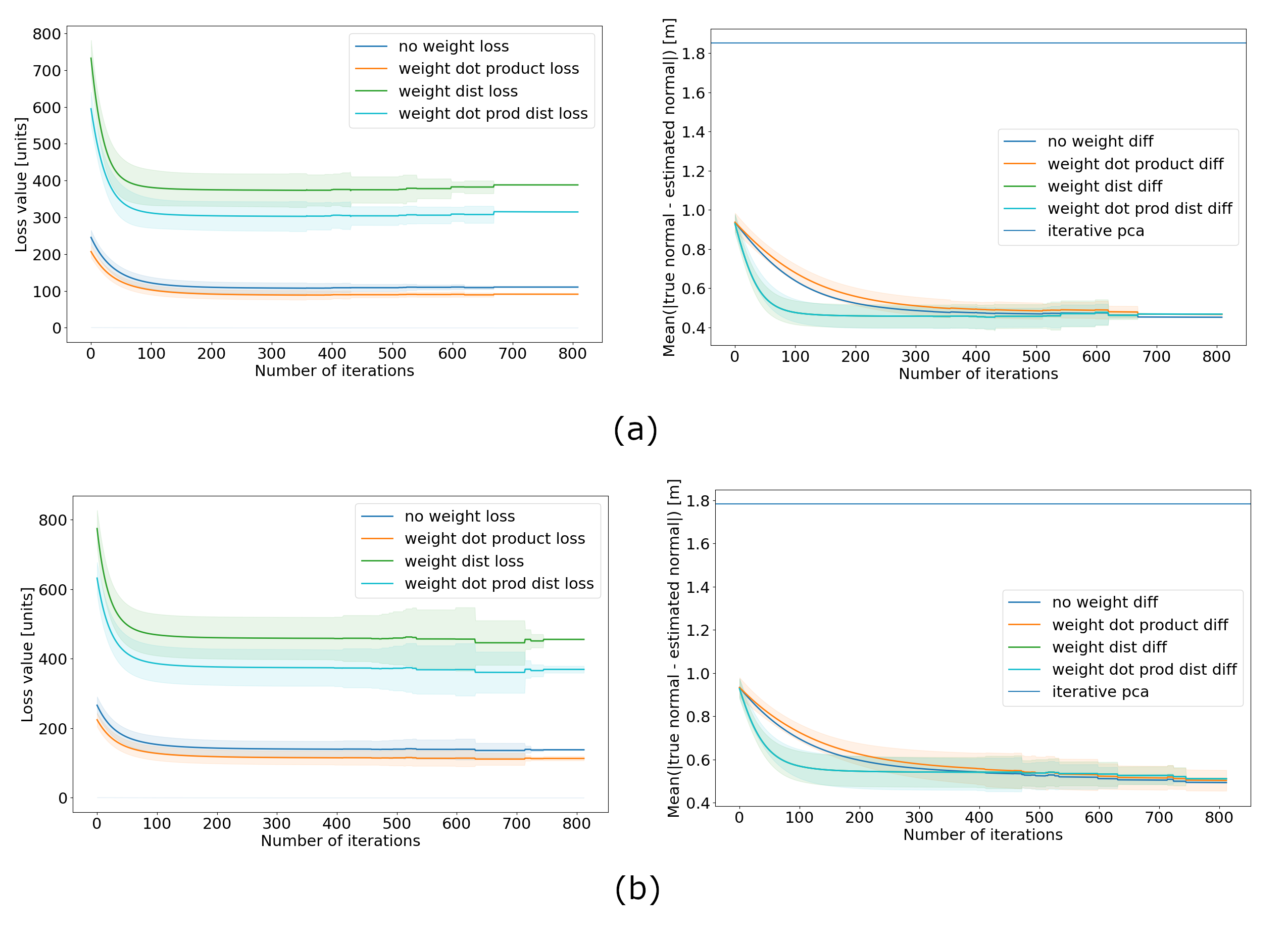
The simulation study is conducted $30$ iterations at each noise level. In each iteration, we generate the dataset, apply the proposed approach to the datasets, and check the estimation performance. To illustrate the estimation uncertainty, we plot both the mean and $\pm 3$ standard deviation (corresponding to the $99\%$ confidence intervals) over the $30$ iterations. We showcase the training loss in Eq.(11) (in the left panels of Fig. 2 and Fig. 3) and the estimation bias of the normals from the ground truth, $\left\|\boldsymbol{\hat{n}}-\boldsymbol{n}\right\|$ (in the right panels of Fig. 2 and Fig. 3). Particularly, we compare the proposed method under the basic optimization setup (referred in the figures as no weight) and under the three weighting strategies (referred in the figures as weight dot prod, weight dist and weight dot prod dist respectively). We compare our proposed approach with our reproduction of the robust normal estimation proposed by [Sanchez et al., 2020] which is illustrated in a horizontal line in the difference plots. The left panels of Fig. 2 and Fig. 3 indicate that the proposed algorithm consistently converges under different choices of weighting strategies. Among them, weighting using a combination of dot product and distance shows a higher convergence speed than the other weighting strategies. The right panels of Fig. 2 and Fig. 3 imply that the weights using a combination of dot product and distance achieves the minimal bias comparing to the other weighting strategies. It is worth noting that the formulation without weighting results in an estimation bias of $1.90$ since the normals near the boundaries between two different surfaces are not correctly estimated. With the weighting strategy using a combination of dot product and distance introduced, the estimation bias is reduced to about $0.30$, demonstrating the necessity of the iterative weighting procedure.

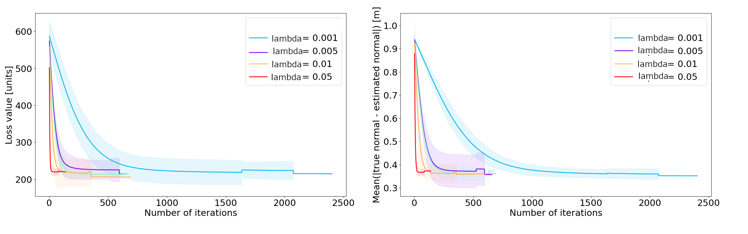
For all the experiments conducted so far, we utilize a constant tuning parameter $\lambda=0.01$. However, in other learning literature (for e.g. [Do et al., 2007]), it has been mentioned that the value of the penalty is more important than the choice of the regularization. In order to understand the effect of the hyperparameter, we perform a grid search for the tuning parameter $\lambda$ over the set $\left\{0.001,0.005,0.01,0.05\right\}$ and showcase the loss values and estimation bias over all iterations for 10 randomly corrupted datasets at each level. The results for the loss and bias using the third weighting strategy for the different tuning parameters at all iterations are given in Fig. 4. The figure suggests to use a $\lambda$ greater than $0.005$ to achieve a low estimation bias. The figure also implies that a higher tuning parameter increases the convergence speed with the highest $\lambda$ value leading to the fastest convergence. This is natural because a higher $\lambda$ sets more regularization on the similarity of the estimated normals in neighboring points, which reduces the efforts in searching for an individual normal for each data point.

The SynPeb dataset was released by [Schaefer et al., 2019] as a comprehensive benchmarking dataset for planar estimation from depth images which got rid of some of the glaring problems of the original planar extraction benchmarking SegComp Perceptron Dataset [Hoover et al., 1996], namely, errors in noise and labeling. Also, SynPeb can provide accurate normal information on account of it being a simulated dataset while being very complex. Although [Hoover et al., 1996] presented a cluster-based normal estimation method and showed a good estimation performance, the estimation procedure highly depends on the quality of clustering, which may not always be high in real applications.

Alternatively, our proposed formulation does not require any prior information on clustering. Given the 3D point clouds, we first apply the proposed method to estimate the normals, compute the pairwise dot products among all the estimated normals, and then directly apply any graph-based clustering method [Schaeffer, 2007] by using the pairwise dot product as the similarity metric between a pair of points. We set the threshold as $0.95$ and consider a pair of points come from the same cluster when their corresponding pairwise dot product exceeds the threshold. We would like to point out that there might be additional noise based on the clustering algorithm chosen for this task but we report the entire error as part of normal estimation (assuming that the clustering algorithm is perfect).

Table 1 provides the results of the SynPeb dataset by the proposed approach and compares it to the state-of-the-art methods that use the same dataset for plane extraction. The table indicates that our proposed approach outperforms the state-of-the-art methods in terms of correct number of points extracted per plane as well as the root mean square error, including the best state-of-the-art method, PPE. On the other hand, the graph Laplacian regularization avoids the excessively large number of segmentations induced by neighboring normals not being similar. Compared to PPE, our proposed method does not constrain the number of planes and does not start with the clustering which can introduce additional error. Of course, as with PPE, the increased accuracy comes at the cost of increased computational speed and spatial complexity.

References

- [Amayo et al., 2018] Amayo, P., Piniés, P., Paz, L. M., Newman, P., 2018. Geometric multi-model fitting with a convex relaxation algorithm. Proceedings of the IEEE Conference on Computer Vision and Pattern Recognition, 8138–8146.
- [Amenta and Bern, 1999] Amenta, N., Bern, M., 1999. Surface reconstruction by Voronoi filtering. Discrete & Computational Geometry, 22(4), 481–504.
- [Dey and Sun, 2006] Dey, T. K., Sun, J., 2006. Normal and feature approximations from noisy point clouds. International Conference on Foundations of Software Technology and Theoretical Computer Science, Springer, 21–32.
- [Do et al., 2007] Do, C. B., Foo, C.-S., Ng, A. Y., 2007. Efficient multiple hyperparameter learning for log-linear models. NIPS, 2007, Citeseer, 377–384.
- [Duda and Hart, 1972] Duda, R. O., Hart, P. E., 1972. Use of the Hough transformation to detect lines and curves in pictures. Communications of the ACM, 15(1), 11–15.
- [Feng et al., 2014] Feng, C., Taguchi, Y., Kamat, V. R., 2014. Fast plane extraction in organized point clouds using agglomerative hierarchical clustering. 2014 IEEE International Conference on Robotics and Automation (ICRA), IEEE, 6218–6225.
- [Fischler and Bolles, 1981] Fischler, M. A., Bolles, R. C., 1981. Random sample consensus: a paradigm for model fitting with applications to image analysis and automated cartography. Communications of the ACM, 24(6), 381–395.
- [Fleishman et al., 2005] Fleishman, S., Cohen-Or, D., Silva, C. T., 2005. Robust moving least-squares fitting with sharp features. ACM transactions on graphics (TOG), 24(3), 544–552.
- [Hoover et al., 1996] Hoover, A., Jean-Baptiste, G., Jiang, X., Flynn, P. J., Bunke, H., Goldgof, D. B., Bowyer, K., Eggert, D. W., Fitzgibbon, A., Fisher, R. B., 1996. An experimental comparison of range image segmentation algorithms. IEEE transactions on pattern analysis and machine intelligence, 18(7), 673–689.
- [Hoppe et al., 1992] Hoppe, H., DeRose, T., Duchamp, T., McDonald, J., Stuetzle, W., 1992. Surface reconstruction from unorganized points. Proceedings of the 19th annual conference on computer graphics and interactive techniques, 71–78.
- [Jordan and Mordohai, 2014] Jordan, K., Mordohai, P., 2014. A quantitative evaluation of surface normal estimation in point clouds. 2014 IEEE/RSJ International Conference on Intelligent Robots and Systems, IEEE, 4220–4226.
- [Joshi and Caputo, 2020] Joshi, U., Caputo, A., 2020. Lidar technology in manufacturing: Think ahead : Social innovation. https://social-innovation.hitachi/en-us/think-ahead/manufacturing/a-simple-solution-for-complex-problems/.
- [Landrieu et al., 2017] Landrieu, L., Mallet, C., Weinmann, M., 2017. Comparison of belief propagation and graph-cut approaches for contextual classification of 3d lidar point cloud data. 2017 IEEE International Geoscience and Remote Sensing Symposium (IGARSS), IEEE, 2768–2771.
- [Lipman et al., 2007] Lipman, Y., Cohen-Or, D., Levin, D., Tal-Ezer, H., 2007. Parameterization-free projection for geometry reconstruction. ACM Transactions on Graphics (TOG), 26(3), 22–es.
- [Mitchell and Mulzer, 2017] Mitchell, J. S., Mulzer, W., 2017. Proximity algorithms. C. D. T. Jacob E. Goodman, Joseph O’Rourke (ed.), Handbook of Discrete and Computational Geometry, Chapman and Hall/CRC.
- [Moosmann et al., 2009] Moosmann, F., Pink, O., Stiller, C., 2009. Segmentation of 3d lidar data in non-flat urban environments using a local convexity criterion. 2009 IEEE Intelligent Vehicles Symposium, IEEE, 215–220.
- [Morvan and Thibert, 2004] Morvan, J.-M., Thibert, B., 2004. Approximation of the normal vector field and the area of a smooth surface. Discrete & Computational Geometry, 32(3), 383–400.
- [Myers and Myers, 1990] Myers, R. H., Myers, R. H., 1990. Classical and modern regression with applications. 2, Duxbury press Belmont, CA.
- [Pauly et al., 2002] Pauly, M., Gross, M., Kobbelt, L. P., 2002. Efficient simplification of point-sampled surfaces. IEEE Visualization, 2002. VIS 2002., IEEE, 163–170.
- [Rubin-Delanchy, 2020] Rubin-Delanchy, P., 2020. Manifold structure in graph embeddings. Advances in Neural Information Processing Systems, 33.
- [Sanchez et al., 2020] Sanchez, J., Denis, F., Coeurjolly, D., Dupont, F., Trassoudaine, L., Checchin, P., 2020. Robust normal vector estimation in 3D point clouds through iterative principal component analysis. ISPRS Journal of Photogrammetry and Remote Sensing, 163, 18–35.
- [Schaefer et al., 2019] Schaefer, A., Vertens, J., Büscher, D., Burgard, W., 2019. A maximum likelihood approach to extract finite planes from 3-D laser scans. 2019 IEEE/RSJ International Conference on Robotics and Automation (ICRA), IEEE.
- [Schaeffer, 2007] Schaeffer, S. E., 2007. Graph clustering. Computer science review, 1(1), 27–64.
- [Shahid et al., 2016] Shahid, N., Perraudin, N., Kalofolias, V., Puy, G., Vandergheynst, P., 2016. Fast robust PCA on graphs. IEEE Journal of Selected Topics in Signal Processing, 10(4), 740–756.
- [Suger et al., 2015] Suger, B., Steder, B., Burgard, W., 2015. Traversability analysis for mobile robots in outdoor environments: A semi-supervised learning approach based on 3d-lidar data. 2015 IEEE International Conference on Robotics and Automation (ICRA), IEEE, 3941–3946.
- [Torr and Zisserman, 2000] Torr, P. H., Zisserman, A., 2000. MLESAC: A new robust estimator with application to estimating image geometry. Computer vision and image understanding, 78(1), 138–156.
- [Toussaint, 1989] Toussaint, G. T., 1989. Some unsolved problems on proximity graphs.
- [Urmson et al., 2008] Urmson, C., Anhalt, J., Bagnell, D., Baker, C., Bittner, R., Clark, M., Dolan, J., Duggins, D., Galatali, T., Geyer, C. et al., 2008. Autonomous driving in urban environments: Boss and the urban challenge. Journal of Field Robotics, 25(8), 425–466.
- [Xu et al., 2017] Xu, Y., Yao, W., Hoegner, L., Stilla, U., 2017. Segmentation of building roofs from airborne LiDAR point clouds using robust voxel-based region growing. Remote Sensing Letters, 8(11), 1062–1071.