A self-consistent systematic optimization of range-separated hybrid functionals from first principles
Abstract
In this communication, we represent a self-consistent systematic optimization procedure for the development of optimally tuned (OT) range-separated hybrid (RSH) functionals from first principles. This is an offshoot of our recent work, which employed a purely numerical approach for efficient computation of exact exchange contribution in the conventional global hybrid functionals through a range-separated (RS) technique. We make use of the size-dependency based ansatz i.e., RS parameter, , is a functional of density, , of which not much is known. To be consistent with this ansatz, a novel procedure is presented that relates the characteristic length of a given system (where exponentially decays to zero) with self-consistently via a simple mathematical constraint. In practice, is obtained through an optimization of total energy as follows: . It is found that the parameter , estimated as above can show better performance in predicting properties (especially from frontier orbital energies) than conventional respective RSH functionals, of a given system. We have examined the nature of highest fractionally occupied orbital from exact piece-wise linearity behavior, which reveals that this approach is sufficient to maintain this condition. A careful statistical analysis then illustrates the viability and suitability of the current approach. All the calculations are done in a Cartesian-grid based pseudopotential (G)KS-DFT framework.
Keywords: Exchange-correlation functional, range-separated hybrid, optimal tuning, Cartesian grid, fundamental gap, fractional occupation.
I Introduction
Throughout the past several decades, density functional theory (DFT) (Hohenberg and Kohn 1964) has been invoked to electronic structure calculations across an unusually wide variety of fields, from organic chemistry to condensed matter physics, as it allows for an accurate quantum mechanical description at a relatively modest computational cost (Cohen et al. 2011; Burke 2012; Becke 2014; Jones 2015). Practical applications of DFT, to a large extent relies on the solution of Kohn-Sham (KS) equation (Kohn and Sham 1965) or generalization (G)KS equation (Seidl et al. 1996). Within such a framework, the interacting many-electron system is mapped onto an effective single-particle one through a local one-body potential, called KS potential, , keeping the ground-state density fixed. In principle, the theory is exact, and has the ability to capture many-body effects completely and uniquely. All the pertinent interactions present in , are included into a single additive exchange-correlation (XC) potential, . It is the functional derivative of XC energy, , which includes Pauli, correlation and the subtle kinetic energy effects, depending only on . However, although the existence and uniqueness of is guaranteed, its exact form still remains elusive.
So in this scenario, needs to be approximated in the so-called density functional approximation (DFA) hoping that they are sufficiently accurate to be useful. Therefore, the practical success of (G)KS-DFT hinges entirely on the existence of suitable DFAs. The commonly used DFAs can be hierarchically categorized as local (spin) density approximation L(S)DA (Kohn and Sham 1965) (containing only), generalized gradient approximation GGA (Becke 1988; Perdew et al. 1996a) (with addition of gradient of electron density, ), and meta-GGA (Tao et al. 2003; Zhao and Truhlar 2008) (with inclusion of Laplacian of density and kinetic energy density, ), the third rung of Jacob’s ladder (Perdew and Schmidt 2000). With additional introduction of exact exchange (EEX) energy, one gets the hybrid functionals (Becke 1993; Perdew et al. 1996b), while incorporation of EEX energy density, , leads to the hyper functionals (Becke 2005; Perdew et al. 2008), residing in the fourth rung of the ladder. Now we also have functionals that go beyond this (to include virtual orbitals), requiring even higher computational cost, and have also been successfully implemented in several quantum chemistry programs (Grimme and Neese 2007; Zhang et al. 2009).
In general, the DFAs experience certain issues regarding (i) piece-wise linearity (PWL) of total energy in the fractional number of particles (Perdew and Wang 1992; Yang et al. 2000) (ii) non-cancellation of spurious Coulomb self-repulsion energythe so-called self-interaction error (SIE) (Perdew and Zunger 1981; Bao et al. 2018) and (iii) asymptotically correct behavior of XC potential at long range (LR) for finite systems (Levy et al. 1984). These three points are not equivalent, but are connected to each other by a certain extent (Kronik and Kümmel 2020). These are very important conditions for developing advanced density functionals, as each of them allows one to avoid different aspects of spurious electron interaction. A very promising area in which the above conditions can be controlled in a satisfactory way is via an optimal tuning (OT) of the range-separated hybrid (RSH) functionals (Kronik and Kümmel 2018; Baer et al. 2010). Generally, these are based on partitioning the Coulomb interaction kernel into a short range (SR) and a LR part, usually through an RS operator, , and an RS parameter, , in the form of
| (1) |
where, represents the complementary RS operator. This was first proposed in (Leininger et al. 1997) in the field of multi-reference configuration interaction, keeping in mind that the dynamical electron correlation hardly affects the LR interactions due to the rapidly decaying features. Here, plays a pivotal role to adjust the contribution of EEX between SR to LR region for a given RS operator. In literature, these two regions are treated separately, depending on the system of interest. In general, the SR region is described using a modified inter-electronic distance-dependent local or semi-local DFA and the LR sector by EEX with the correction, mainly in the finite systems. The XC energy, based on above partitioning scheme then can be defined as,
| (2) |
where , refer to EEX energy contribution while , denote DFA exchange, at SR and LR regions respectively. A particular set of (, ) defines a specific mode of partitioning for a given . RSH functionals with make XC potential asymptotically correct at LR region. At the same time, a delicate balance between EEX and dynamical correlation is retained by adopting an optimal value of . Hence, these functionals are not fully SIE free. Moreover, they do not follow the PWL condition unless optimally tuned of a given system. This is due to the default value of , which is usually obtained semi-empirically by fitting the reference data (Iikura et al. 2001; Tawada et al. 2004; Yanai et al. 2004; Lange et al. 2008).
In OT procedure, is usually determined from first principles by actively enforcing Koopmans’ theorem (Salzner and Baer 2009). It satisfies PWL conditions, and in principle, would preserve the size-dependency of on , but is very hard to maintain with a universal value of (Baer et al. 2010). It makes the XC potential asymptotically correct at LR region. This improves properties based on orbital energies, such as vertical ionization energy (IE), electron affinity (EA), fundamental gap (FG), optical gap, charge-transfer excitation as well as Rydberg excitation (Livshits and Baer 2007; Stein et al. 2010). Besides the traditional -tuning scheme based on satisfying Koopmans’ theorem, recent advances based on electron localization function and localized orbital locator have been developed in the literature which requires only one single self-consistent field calculation (Borpuzari and Kar 2017; Wang and Zhang 2018). Moreover, a self-consistent OT-RSH approach (Tamblyn et al. 2014) has been developed based on the minimization of inter-atomic forces, which offers better geometries and vibrational modes.
These developments motivated us to work further in this area by asking “how else one can self-consistently and systematically optimize for a given system from first principles irrespective of the properties of interest”. That lies at the heart of constructing ab initio OT-RSH functionals. Here, we present such a procedure, taking inspiration from our recent work published elsewhere (Ghosal et al. 2019), where we pursued a fully numerical approach for efficient computation of EEX contribution. A size-dependency based ansatz is invoked i.e., is a functional of density. Thus a systematic procedure is presented that relates with via a simple mathematical constraint following the arguments of (Ghosal and Roy 2016; Ghosal et al. 2018; Ghosal et al. 2019). In practice, we obtain through an optimization of total energy as follows: . The suitability, efficacy and performance of this is analyzed by a comparison of certain properties derived from orbital energies. Next, we have examined the nature of highest fractionally occupied orbital from exact PWL behavior. Moreover, we also consider small chains versus small conjugated molecules to reveal the effect of conjugation in determining . At the end, a comparison between present method with the traditional OT strategy is discussed.
The manuscript is organized as follows. In next section, we briefly review the general framework of Cartesian coordinate grid (CCG) based pseudopotential (G)KS-DFT. Then, we present the theoretical background for SR/LR-EEX through Fourier convolution theorem (FCT) in CCG. Next, we discuss in detail about optimal tuning of . In Sec. III, computational details are given. In Sec. IV, we illustrate the performance of proposed scheme considering following properties such as IE, EA, FG and fractional occupation for a decent number of atoms () and molecules (20). These are presented for LC-BLYP, CAM-B3LYP, LC-PBE, CAM-PBE0, LRC-PBEh⋆ functional along with their presently described OT version (denoted by “ot” subscript), as well as global hybrids B3LYP and PBE0 functionals. Finally, conclusions as well as future and outlook are summarized in the last section.
II Methodology
II.1 Pseudopotential (G)KS-DFT in CCG
For a many-electron system, one can write the single-particle (G)KS equation in presence of pseudopotential as (atomic unit employed unless stated otherwise),
| (3) |
where denotes the ionic pseudopotential, written as below,
| (4) |
In the above equation, signifies ion-core pseudopotential associated with atom A, situated at . The classical Coulomb (Hartree) term, describes usual electrostatic interaction amongst valence electrons whereas signifies the non-classical XC part of latter, and corresponds to a set of occupied orthonormal spin-MOs. Within LCAO-MO approximation, the coefficients for expansion of spin-MOs satisfy a set of equations, very similar to that in HF theory,
| (5) |
satisfying the orthonormality condition, . Here contains the respective spin-MO coefficients for a given spin-MO , is the usual overlap matrix corresponding to elements , refers to diagonal matrix of spin-MO eigenvalues . The (G)KS-Fock matrix has elements , constituting of following contributions,
| (6) |
In this equation, all one-electron contributions, such as kinetic energy, nuclear-electron attraction and pseudopotential matrix elements are included in first term, whereas and account for classical Hartree and XC potentials with EEX respectively.
Now we discretize various quantities like localized basis function, electron density, MO as well as two-electron potentials directly on a 3D cubic box having axes,
| (7) |
where denote grid spacing and total number of points along each directions respectively. The electron density in this grid may be simply written as (“g” symbolizes discretized grid),
| (8) |
where corresponds to atomic orbitals (AOs). At this stage, the two-electron contributions of KS matrix are computed through direct numerical integration in the grid,
| (9) |
where refers to the combined Hartree and XC potential. The detailed construction of various potentials in CCG has been well documented in our earlier work (Roy 2008a; Roy 2008b; Roy 2010; Roy 2011; Roy 2009; Ghosal and Roy 2016; Ghosal et al. 2018); hence not repeated here.
II.2 SR/LR exact exchange through FCT
A well-defined numerical methodology for the EEX energy and potential was recently developed in our group (Ghosal et al. 2019). Accordingly the SR/LR EEX energy, , can be computed numerically by integrating the corresponding density as given by,
| (10) |
Now, can be defined as
| (11) |
where is the respective RS operator for a given functional. The two expressions are defined in terms of (G)KS occupied MOs and AOs . The complex conjugate sign is omitted here since the density matrix and basis are generally in real form. This definition of is similar to the EEX energy density evaluation; only the four-center electron repulsion integrals are modified by RS operator.
At first glance, it seems to be computationally expensive due to the fact that it needs to be evaluated at each grid point with four AO indices. But, the scheme in (Ghosal et al. 2019) shows promise in substantial computational cost reduction. Accordingly Eq. (11) can be recast in the following form,
| (12) |
One may anticipate the construction of in three steps of comparable computational cost. The first quantity may be represented as follows:
| (13) |
in which the density matrix is combined with AOs through a simple matrix multiplication. The computational scaling of this step is , with , denoting total number of grid points and number of AO basis functions. The next crucial (rate-determining) step is to evaluate the SR/LR two-center electrostatic potential (ESP) integral which is embedded in and can be defined as,
| (14) |
The scaling cost of this integral is . Usually one may perform this integral analytically using primitive functions and different types of recursion algorithms, such as Obara-Saika (Obara and Saika 1986; Obara and Saika 1988), Head-Gordon-Pople (Head-Gordon and Pople 1988) or their combination (Liu et al. 2016). Here, we perform FCT for accurate estimation of this integral, which is discussed in the following.
The final step consists of computation of the quantity in accordance with the following expression:
| (15) |
The step involves same scaling, as the ESP integral evaluation, but requires fewer steps than latter; needing only one multiplication and one addition at innermost loop. This also effectively provides a purely numerical way to compute the LR/SR exact exchange matrix, , which according to Eqs. [11-13] can be rewritten as,
| (16) |
Now the two-center SR/LR ESP integral, which is the core computing component, can be rewritten as,
| (17) |
The last expression is in terms of convolution integral, where denotes simple multiplication of two AO basis functions and represents the modified Coulomb interaction kernel by a given RS operator. Now one can invoke FCT to further simplify this integral,
| (18) |
Here, and stand for fast Fourier transformation (FFT) and inverse FFT, respectively, and and denote Fourier integrals of the modified Coulomb kernel and AO basis functions respectively. From the foregoing discussion, it is evident that each ESP integral involves only a combination of FFT (two forward and one backward transformation simultaneously) leading to scaling. Here, the computational cost remains independent of degree of contraction, and apart from pre-factors, , each ESP integral becomes logarithmic. This could be advantageous for basis sets with large degrees of contraction, for a system requiring moderate grid size. A detailed analysis including real-time performance of present approach with commonly used Gaussian basis functions, has already been enumerated in (Ghosal et al. 2019), and hence not repeated here.
Similarly, the SR/LR EEX energy and its contributions towards (G)KS-Fock matrix can be computed numerically in CCG as:
| (19) |
II.3 Optimal tuning of from first principles
Let us consider an atom A with ground-state density with and similarly for an atom B. When both the atoms are taken together at infinite separation, then density of the composite system will be considering is very large. Then the system too has a RS parameter . That is no longer possible using a universal . Traditionally, the common RSH functionals with fixed break the size-dependency of total energy. Therefore, should depend on system’s size or more specifically be a functional of , and it has been confirmed both from formal consideration (Baer and Neuhauser 2005) and practical simulation for the homogeneous electron-gas problem (Livshits and Baer 2007). Moreover, it has been proposed (Stein et al. 2010) that a high level of performance can be achieved if one treats as a system-dependent parameter tuned from first principles. The great advantage of OT is that it preserves the size dependency.
Here we argue that it is possible to estimate systematically by optimizing the total energy of a given system. In (Ghosal and Roy 2016; Ghosal et al. 2018; Mandal et al. 2019; Ghosal et al. 2019), we have shown that within a CCG framework, for each combination of , , , we have the self-consistent field (SCF) density and total energy of a given system after solving Eq. (3). Thus, we can easily write as,
| (20) |
where “i” stands for ith combination of , , with fixed . Further, for a given , one can find out an optimal value of such that,
where the is the grid accuracy for total energy convergence i.e., the energy difference between two successive calculations with different , and . Furthermore, each combination of , where , actually defines the optimal length of the simulation box at each direction. Among them, the smallest one, defined as the minimum length, where exponentially decays to zero, becomes the characteristic length of a given system (Leininger et al. 1997).
Now for a given grid parameter, can be fixed through a mathematical constraint, similar to that used in (Ghosal and Roy 2016; Ghosal et al. 2018; Mandal et al. 2019; Ghosal et al. 2019) in the context of Hartree potential and EEX contribution,
| (21) |
where, refers to the smallest length of the simulation box. This expression is rather more empirical than from physical grounds. It connects the physical parameter , which is local in nature, with the numerical parameter . Note that will change if the numerical grid parameter is changed, which in turn, will modify . Moreover, the SCF density will alter for a variation in , which will again modify . This prompts us to write,
| (22) |
Hence, each combination of , , will fix , and consequently . Accordingly, one can find the SCF density and total energy of a given system for this particular .
It inscribes formally the size dependency of for a given system through the self-consistent density and consequently, with the total energy of that system. Now, an optimization of the total energy with respect to grid parameters gives the characteristic length of a given system, and hence from Eq. (21). Therefore,
| (23) |
Here, we have not made use of any fitting procedure for , with experimental results. Each system has its own characteristic length (Leininger et al. 1997) and, therefore, the current procedure satisfies size dependency principle. It is itself sufficient to obtain the characteristic length, and hence, the optimal value of . This offers a simple machinery to estimate directly in an RSH functionals from first principles.
It is to be noted that Eq. (23) provides a rather general mapping rule. Though, it is trivial to compute the characteristic length, in CCG, its generalization towards other frameworks is highly demanding. Through out the optimization procedure, we have kept fixed and the factor in Eqs. (21) and (23). As pointed out in (Körzdörfer et al. 2011), the primary effect of is to control the length scale for range separation, i.e., the screening of Coulomb interaction, in a particular system of interest. However, since has to reflect Coulomb screening, it can be expected to be sensitive to the size and electronic structure of the system under consideration. The formal justification of Eq. (21) is well documented in (Martyna and Tuckerman 1999) in the context of treating long-range interactions in ab initio and force-field-based calculations in clusters. This is based on a convergent relationship between the expressions for long-range forces in an infinitely replicated periodic system and those in a finite system. It basically “screens” the interaction of the system with an infinite array of periodic images. They defined the screening function with a convergent parameter that controlled the range of interaction, and ensures that the error due to replicated periodic images in a finite system can be neglected. Here, we have redefined it in the desired context of exact long-range exchange of RSH functionals, based on the fact that we also used the same receiprocal based method to treat long-range interaction in a simulation box of finite length. Then, we have made an attempt to connect it through the characteristic length of a given system. Moreover, it has been well demonstrated that for a screening (convergence) function like , the choice of yields accurate results for a wide variety of systems where, denotes the smallest size of simulation box. At the same time, it allows efficient numerical integration on the Cartesian grid. However our practical experience (Ghosal and Roy 2016; Ghosal et al. 2018; Mandal et al. 2019; Ghosal et al. 2019) suggests to be an optimal condition in terms of cost and accuracy.
Note that, the OT as devised in (Livshits and Baer 2007; Stein et al. 2010; Tamblyn et al. 2014; Kronik et al. 2012), for the standard OT-RSH functionals, is generally seen as estimating from first principles. The basic difference of our representation and standard OT-RSH is as follows: our representation is completely different from their work requiring calculation only on neutral species and the optimization of total energy with respect to grid parameters. On the other hand, standard OT-RSH functionals used Koopmans’ theorem and PWL condition on both neutral and charged species (corresponding cation and anion) requiring several calculations on whole range of for the properties derived from orbital energies. We believe that our representation may be useful in the future development of ab initio OT-RSH functionals.
III Computational details
The general framework of RSH functionals is defined in Eq. (2), and in this rubric, we consider three well-established mode of partitioning. The first one, long-range correction (LC) scheme (Iikura et al. 2001) is represented as:
| (24) |
The second one is that of Coulomb-attenuating method (CAM) approach (Yanai et al. 2004) which was introduced using a more general form of RS operator as:
| (25) |
The parameter allows incorporation of EEX contribution over the whole range by a factor of , while leads to inclusion of DFA in the entire range by a factor of . In the special case, CAM approach leads to LC with . These two parameters are connected to in a complicated manner. The last one, we consider here, is the so-called long-range-corrected (LRC) approach (Rohrdanz et al. 2009), having an extra parameter for as:
| (26) |
This parameter allows to incorporate a desired amount of by a factor of . In special case, the LRC approach with leads to LC. A variety of other partitioning schemes including different RS operators have also been explored in the literature (Chai and Head-Gordon 2008a; Chai and Head-Gordon 2008b; Peverati and Truhlar 2012; Vikramaditya et al. 2018; Chan et al. 2019), mainly in connection with thermochemistry and reaction barrier heights.
An important aspect of RSH functionals is the successful development of . Several schemes have been proposed in the past, such as, based on model exchange hole (Iikura et al. 2001; Henderson et al. 2008), adiabatic connection theorem (Baer and Neuhauser 2005; Cohen et al. 2007), exchange energy density (Chai and Head-Gordon 2008b; Lin et al. 2012). Here, we have used the formulation of (Iikura et al. 2001), applicable to any LDA or GGA type DFAs, which involves modified Fermi wave vector in exchange enhancement factor. This was later adopted to develop CAM-B3LYP functional (Yanai et al. 2004) using a more general form of RS operator as defined in Eq. (25). Accordingly, the SR GGA-exchange energy can be cast as:
| (27) |
where, is the usual enhancement factor. The average relative momentum for GGA, is used to define the modified GGA-enhancement factor, . It is easily seen that Eq. (27) reproduces the original GGA DFAs for . The corresponding potential is evaluated using the modified GGA-enhancement factor as it was done for standard GGA DFAs (Johnson et al. 1993). Further development of more balanced SR DFAs can be found in (Iikura et al. 2001; Henderson et al. 2008; Baer and Neuhauser 2005; Cohen et al. 2007; Chai and Head-Gordon 2008b; Lin et al. 2012). Note that, the original LRC scheme was proposed based on Perdew-Burke-Ernzerhof (PBE) exchange hole, which satisfies the above constraints (Ernzerhof and Perdew 1998) at all .
The three distinct kind of RSH functionals (LC, CAM and LRC) as mentioned above are used in our calculations keeping the mode of partitioning and RS operator fixed as in the original articles. As mentioned earlier, the default values of , and other auxiliary parameters () were obtained semi-empirically by fitting the reference data. Here, however, we follow the strategy of Sec. II to determine . These are implemented in case of five representative set of functionals containing a variable amount of SR/LR exact exchange with SR DFA exchange and conventional correlation functional in our in-house pseudopotential (G)KS-DFT program in CCG, InDFT (A. K. Roy, A. Ghosal and T. Mandal 2019). We consider the LC-BLYP (Tawada et al. 2004) and LC-PBE (Iikura et al. 2001; Perdew et al. 1996a) functionals from LC-hybrid group with and , respectively. Moreover, CAM-B3LYP (Yanai et al. 2004) employing , and CAM-PBE0 (Lange et al. 2008) with , are used for CAM-hybrid group. The original LRC-PBEh functional (Rohrdanz et al. 2009) with , is used for LRC-hybrid group with slight modification. Here, it is denoted as LRC-PBEh⋆. It is superscripted with a to differentiate from the original. The only difference is about the construction of SR DFA-exchange. In (Rohrdanz et al. 2009), it is based on PBE exchange hole. In present work, we have used the procedure from one-particle density matrix, as we done for LC and CAM categories, to make them consistent with each other. All the parameters except are kept fixed as in the original article, and these functionals are denoted with the subscript “ot”. Two global hybrid functionals, namely, B3LYP, and PBE0, containing a variable amount of EEX energy with a conventional DFA are also considered side by side (Stephens et al. 1994; Perdew et al. 1996b).
| Set I | Set II | |||||||
|---|---|---|---|---|---|---|---|---|
| 32 | 32 | 32 | 15.48226 | 32 | 36 | 60 | 15.50095 | |
| – | – | 36 | 15.49414 | 32 | 44 | – | 15.50175 | |
| – | – | 40 | 15.49695 | 32 | 48 | – | 15.50175 | |
| – | – | 44 | 15.49760 | 32 | 52 | – | 15.50178 | |
| – | – | 48 | 15.49775 | 32 | – | – | 15.50178 | |
| – | – | 52 | 15.49777 | 36 | – | – | 15.50495 | |
| – | – | 56 | 15.49778 | 44 | – | – | 15.50575 | |
| – | – | 60 | 15.49778 | 48 | – | – | 15.50578 | |
| – | – | 64 | 15.49778 | 52 | – | – | 15.50578 | |
| †Energy from GAMESS package Schmidt et al. 1993: 15.50592 a.u. |
We employ following effective core potential (ECP) basis sets: SBKJC (Stevens et al. 1984) for species containing Group-II elements and LANL2DZ (Hay and Wadt 1985) for Group-III or higher group elements. These are adopted from EMSL Basis Set Library (Feller 1996). All one-electron integrals are generated by standard recursion relations (Obara and Saika 1986) using Cartesian Gaussian-type orbitals as primitive basis functions. The norm-conserving pseudopotential matrix elements in contracted basis are imported from GAMESS (Schmidt et al. 1993) suite of program package. The relevant LDA- and GGA-type of functionals in connection with B3LYP, and PBE0 are: (i) Vosko-Wilk-Nusair (VWN)–with the homogeneous electron gas correlation proposed in parametrization formula V (Vosko et al. 1980) (ii) B88–incorporating Becke (Becke 1988) semi-local exchange (iii) Lee-Yang-Parr (LYP) (Lee et al. 1988) semi-local correlation (iv) PBE (Perdew et al. 1996a) for semi-local exchange and correlation. The modified SR-exchange B88 from Eq. (27) and LYP correlation are invoked for LC-BLYP and CAM-B3LYP, whereas the modified SR-exchange PBE from Eq. (27) and PBE correlation for LC-PBE, CAM-PBE0, LRC-PBEh⋆. All correlation functionals are directly adopted from density functional repository program (rep 2001). The convergence criteria imposed in this communication are slightly tighter than our earlier work (Roy 2008a; Roy 2008b; Roy 2010; Roy 2011); this is to generate a more accurate orbital energy. Changes in following quantities were followed during the SCF process, viz., (i) orbital energy difference between two successive iterations and (ii) absolute deviation in a density matrix element. They both are required to remain below a prescribed threshold set to a.u.; this ensured that total energy maintained a convergence of at least this much, in general. In order to perform discrete Fourier transform, standard FFTW3 package (Frigo and Johnson 2005) is invoked. The resulting generalized matrix-eigenvalue problem is solved through standard LAPACK routine (Anderson et al. 1999) accurately and efficiently. All molecular calculations are performed in their experimental geometries, taken from NIST database (Johnson 2016). Other details including scaling properties may be found in references (Roy 2008a; Roy 2008b; Roy 2010; Roy 2011; Ghosal and Roy 2016; Ghosal et al. 2018; Mandal et al. 2019; Ghosal et al. 2019; Ghosal et al. 2021).
| Set I | Set II | |||||||
|---|---|---|---|---|---|---|---|---|
| 32 | 32 | 32 | 11.14114 | 32 | 40 | 60 | 11.17356 | |
| – | – | 36 | 11.15210 | 32 | 44 | – | 11.17456 | |
| – | – | 40 | 11.15508 | 32 | 52 | – | 11.17486 | |
| – | – | 44 | 11.15583 | 32 | 56 | – | 11.17487 | |
| – | – | 48 | 11.15600 | 32 | 60 | – | 11.17487 | |
| – | – | 52 | 11.15604 | 36 | – | – | 11.18494 | |
| – | – | 56 | 11.15605 | 48 | – | – | 11.18850 | |
| – | – | 60 | 11.15606 | 56 | – | – | 11.18855 | |
| – | – | 64 | 11.15606 | 60 | – | – | 11.18855 | |
| †Energy from GAMESS package Schmidt et al. 1993: 11.18865 a.u. |
IV Results and discussion
Before proceeding for main results, it may be appropriate first to discuss the grid optimization on the convergence of total energy, , which plays a vital role for practical implementation of Eq. (23). For illustration, we choose two RSH functionals, namely, CAM-B3LYP and LC-BLYP. All the calculations presented in this section are performed through our in-house pseudopotential (G)KS-DFT program in CCG (A. K. Roy, A. Ghosal and T. Mandal 2019). At first, Table I shows this for CAM-B3LYP for HCl at its experimental geometry (bond length Å). The total energy is provided in non-uniform grid with respect to sparsity (regulated by ) for a fixed grid spacing (determined by , chosen as 0.3), employing fixed parameter , and from Eq. (25). Following our previous works (Ghosal and Roy 2016; Ghosal et al. 2018; Ghosal et al. 2019) we first vary , the number of grid points along inter-nuclear axis, keeping the same along plane static at certain reasonable value, say . As is gradually increased from 32 to 64 with an increment of 4, there is a smooth convergence in energy at around , with a difference (we term it as grid accuracy) of about a.u., between two successive steps. In the beginning, when goes through , one notices slow improvement in energy; after that it eventually attains the convergence for at around for a particular value of grid accuracy. Then in Set II in right-hand side, we vary sequentially and along plane keeping first and fixed at its previously determined value of and respectively, and then vary keeping and fixed at and respectively. Now we can see that the convergence in energy takes place at and with same grid accuracy of Set I. For sake of completeness, the respective energy is also quoted from GAMESS Schmidt et al. 1993 in footnote. Next we move toward the implementation of LC-BLYP using the same procedure mentioned above. For this, we consider a non-linear triatomic molecule H2S as a specimen case. The stability of our current implementation through the total energy convergence is illustrated in Table II at a grid spacing of using the same convergence criteria as imposed in Table I. Here also the respective energy value is quoted from GAMESS in footnote. The performance of our calculated energies from Tables I and II are quite accurate with the reference results for a given grid accuracy.
| Atom | B3LYP | LC-BLYP | LC-BLYPot | CAM-B3LYP | CAM-B3LYPot | PBE | LC-PBE | LC-PBEot | CAM-PBE | CAM-PBEot | LRC-PBEh⋆ | LRC-PBEh⋆ot | Expt.† |
| Be | 6.23 | 8.52 | 8.50 | 7.64 | 7.63 | 6.50 | 8.58 | 8.67 | 8.71 | 8.78 | 8.23 | 8.75 | 9.32 |
| B | 4.98 | 7.55 | 7.85 | 6.63 | 6.77 | 5.25 | 7.45 | 7.93 | 7.79 | 8.16 | 7.06 | 8.11 | 8.30 |
| C | 7.12 | 9.88 | 10.67 | 8.96 | 9.32 | 7.54 | 9.79 | 10.65 | 10.39 | 11.04 | 9.43 | 10.96 | 11.26 |
| N | 9.52 | 12.27 | 13.53 | 11.47 | 12.05 | 10.09 | 12.22 | 13.79 | 13.12 | 14.30 | 11.98 | 14.20 | 14.53 |
| O | 8.83 | 11.42 | 12.97 | 10.77 | 11.49 | 9.19 | 11.13 | 13.00 | 12.10 | 13.50 | 10.95 | 13.40 | 13.62 |
| Al | 3.51 | 5.59 | 5.63 | 4.79 | 4.81 | 3.83 | 5.74 | 5.87 | 5.87 | 5.96 | 5.46 | 6.09 | 5.99 |
| Si | 5.27 | 7.67 | 7.72 | 6.78 | 6.80 | 5.68 | 7.81 | 8.01 | 8.06 | 8.22 | 7.46 | 8.18 | 8.15 |
| P | 6.93 | 9.46 | 9.77 | 8.57 | 8.71 | 7.43 | 9.63 | 10.13 | 10.03 | 10.40 | 9.29 | 10.35 | 10.49 |
| S | 6.82 | 9.37 | 9.82 | 8.49 | 8.69 | 7.14 | 9.34 | 10.00 | 9.75 | 10.24 | 8.97 | 10.19 | 10.36 |
| Cl | 8.96 | 11.63 | 12.37 | 10.75 | 11.10 | 9.36 | 11.58 | 12.57 | 12.17 | 12.92 | 11.25 | 12.85 | 12.97 |
| Ga | 3.44 | 5.49 | 5.53 | 4.71 | 4.72 | 3.76 | 5.65 | 5.78 | 5.77 | 5.87 | 5.37 | 5.85 | 6.00 |
| Ge | 4.97 | 7.27 | 7.32 | 6.41 | 6.43 | 5.37 | 7.44 | 7.62 | 7.66 | 7.79 | 7.12 | 7.76 | 7.90 |
| As | 6.60 | 9.05 | 9.22 | 8.17 | 8.24 | 7.09 | 9.24 | 9.57 | 9.57 | 9.82 | 8.91 | 9.77 | 9.82 |
| Se | 6.36 | 8.83 | 9.10 | 7.94 | 8.06 | 6.67 | 8.84 | 9.28 | 9.15 | 9.49 | 8.47 | 9.47 | 9.75 |
| Br | 8.19 | 10.78 | 11.10 | 9.87 | 10.02 | 8.56 | 10.77 | 11.30 | 11.20 | 11.60 | 10.41 | 11.54 | 11.81 |
| MAE | 3.50 | 1.03 | 0.61 | 1.89 | 1.69 | 3.12 | 1.00 | 0.41 | 0.60 | 0.15 | 1.33 | 0.20 | |
| ME | 3.50 | 1.03 | 0.61 | 1.89 | 1.69 | 3.12 | 1.00 | 0.41 | 0.60 | 0.15 | 1.33 | 0.19 | |
| 1.69 | 1.12 | 2.44 | 4.00 | 6.65 |
| †Optical spectroscopy (Johnson 2016). | ‡: Ratio between MAE value of RSH and OT-RSH. |
To broaden the scope of applicability, we now focus on certain properties derived from frontier orbital energies. Henceforth we use the same grid optimization procedure through Eq. (23) maintaining the same grid accuracy of Tables I and II. To put things in perspective, we categorize the five functionals into two distinct blocks (B3LYP and PBE0) such that those RSH functionals containing “B88” exchange and “LYP” correlation belong to B3LYP and those including “PBE” exchange and correlation belong to PBE0 block. Moreover, the mean absolute error (MAE) and mean error (ME) from statistical analysis have been provided to facilitate a detailed comparison with the available ab initio/experimental results.
IV.1 Ionization energies
The physical interpretation of KS frontier orbital and its energies as single-particle quantities is still far from straightforward, even if we know the exact XC potential, except the highest occupied molecular orbital (HOMO). It can be assigned using the “KS analogue of Koopmans’ theorem in Hartree-Fock theory” (Perdew et al. 1982; Levy et al. 1984; Perdew and Levy 1997) and accordingly, one can write as,
| (28) |
where, IE() be the first ionization energy of a given -electron system. In the context of LDA or GGA-type DFAs, Eq. (28) is no longer be a valid statement; the HOMO energy is usually underestimated. Moreover, this will not work for other functionals outside of KS regime, particularly in which we are interested in this communication. The RSH functionals, in principle, have correct asymptotic behavior at LR region, but the essence of HOMO and its energy is possible only through (G)KS version of Koopmans’ theorem. It has been proved that for the specific case of an EEX operator, it is still possible to identify the (G)KS HOMO energy with (Görling and Levy 1997), and accordingly
| (29) |
. Like KS mapping, the (G)KS map is not unique, and considering RSH functional, any choice of generates a legitimate approximate (G)KS map. The obvious question is then, whether RSH functionals with fixed values of can approximate (G)KS HOMO energy accurately with , irrespective of systems of interest? Therefore, the comparison of the (G)KS HOMO energy with experimental is a good test in determining through Eq. (23).
| System | B3LYP | LC-BLYP | LC-BLYPot | CAM-B3LYP | CAM-B3LYPot | PBE | LC-PBE | LC-PBEot | CAM-PBE | CAM-PBEot | LRC-PBEh⋆ | LRC-PBEh⋆ot | Expt.† |
| N2 | 11.48 | 14.25 | 14.81 | 13.45 | 13.71 | 11.83 | 13.94 | 14.82 | 14.88 | 15.54 | 13.71 | 15.40 | 15.60 |
| Si2 | 5.71 | 7.91 | 7.90 | 7.09 | 7.08 | 6.03 | 8.10 | 8.16 | 8.21 | 8.26 | 7.82 | 8.24 | 7.90 |
| P2 | 7.89 | 10.33 | 10.50 | 9.46 | 9.54 | 8.23 | 10.33 | 10.69 | 10.70 | 10.97 | 10.01 | 10.92 | 10.62 |
| S2 | 6.66 | 8.49 | 8.69 | 7.59 | 7.69 | 7.06 | 8.45 | 8.86 | 8.91 | 9.21 | 8.11 | 9.14 | 9.40 |
| Cl2 | 8.55 | 11.21 | 11.78 | 10.34 | 10.60 | 8.98 | 11.18 | 11.99 | 11.79 | 12.40 | 10.87 | 12.32 | 11.48 |
| CO | 10.30 | 13.10 | 13.58 | 12.21 | 12.44 | 10.60 | 12.82 | 13.59 | 13.56 | 14.14 | 12.49 | 14.03 | 14.10 |
| NaCl | 5.79 | 8.37 | 7.67 | 7.44 | 7.12 | 6.12 | 8.33 | 7.81 | 8.79 | 8.45 | 8.26 | 8.33 | 9.80 |
| HCl | 8.91 | 11.60 | 12.35 | 10.71 | 10.98 | 9.32 | 11.55 | 12.54 | 12.15 | 12.90 | 11.22 | 12.83 | 12.79 |
| CO2 | 10.30 | 13.10 | 13.58 | 12.21 | 12.44 | 10.61 | 12.82 | 13.59 | 13.56 | 14.14 | 12.49 | 14.03 | 14.10 |
| H2O | 8.26 | 10.97 | 11.51 | 10.21 | 10.45 | 8.63 | 10.71 | 11.55 | 11.65 | 12.28 | 10.51 | 12.14 | 12.62 |
| H2S | 7.12 | 9.77 | 10.11 | 8.84 | 8.99 | 7.48 | 9.74 | 10.29 | 10.18 | 10.60 | 9.37 | 10.54 | 10.48 |
| C2H2 | 7.94 | 10.72 | 11.04 | 9.68 | 9.83 | 8.33 | 10.71 | 11.24 | 11.08 | 11.47 | 10.28 | 11.42 | 11.40 |
| NH3 | 6.65 | 9.39 | 9.86 | 8.53 | 8.75 | 7.02 | 9.21 | 9.96 | 9.95 | 10.51 | 8.92 | 10.40 | 10.82 |
| PH3 | 7.25 | 9.77 | 9.96 | 8.88 | 8.97 | 7.55 | 9.72 | 10.10 | 10.11 | 10.40 | 9.37 | 10.34 | 9.89 |
| CH4 | 10.48 | 13.19 | 13.78 | 12.30 | 12.57 | 10.85 | 13.06 | 13.91 | 13.68 | 14.32 | 12.73 | 14.24 | 13.6 |
| CH3Cl | 8.02 | 10.67 | 11.04 | 9.76 | 9.94 | 8.39 | 10.60 | 11.20 | 11.14 | 11.59 | 10.27 | 11.51 | 11.29 |
| SiH4 | 9.71 | 12.28 | 12.37 | 11.40 | 11.44 | 10.02 | 12.19 | 12.49 | 12.65 | 12.88 | 11.84 | 12.80 | 12.30 |
| C2H4 | 7.27 | 10.00 | 10.18 | 8.95 | 9.03 | 7.67 | 10.06 | 10.41 | 10.34 | 10.60 | 9.62 | 10.56 | 10.51 |
| C2H6 | 9.12 | 11.71 | 11.95 | 10.86 | 10.97 | 9.46 | 11.59 | 12.06 | 12.16 | 12.52 | 11.28 | 12.43 | 11.99 |
| Si2H6 | 8.23 | 10.62 | 10.59 | 9.76 | 9.74 | 8.54 | 10.62 | 10.75 | 10.94 | 11.04 | 10.30 | 10.98 | 10.53 |
| MAE | 3.28 | 0.70 | 0.47 | 1.58 | 1.45 | 2.93 | 0.80 | 0.44 | 0.43 | 0.38 | 1.09 | 0.37 | |
| ME | 3.28 | 0.69 | 0.40 | 1.58 | 1.45 | 2.93 | 0.77 | 0.26 | 0.24 | -0.15 | 1.09 | -0.07 | |
| 1.49 | 1.09 | 1.8 | 1.13 | 2.95 |
| †Photo-electron spectroscopy (Johnson 2016). | ‡: Ratio between MAE value of RSH and OT-RSH. |
To evaluate the performance of our approach on (G)KS HOMO energy, we consider 15 atoms and 20 molecules in our dataset; such molecules are taken from G1 database (Pople et al. 1989). The calculated negative (G)KS HOMO energies for 12 functionals (considering B3LYP and PBE0 blocks) including experimental from NIST database (Johnson 2016) are collected in Tables III and IV. A glance at both MAE and ME of Table III, reveals that these are more or less close to each other for all functionals and also having a positive ME. These clearly indicate an underestimation of IE from the experimental values. But, at the same time, these also provide a scope to further reduce the error systematically within our proposed scheme, which is discussed later. Now, the fruitfulness of OT-RSH functionals is reflected through , a ratio of MAE between RSH and its respective OT-RSH counterpart. The value of for all five functionals are quoted in Table III. Accordingly, LRC-PBEh⋆ot has the largest value of i.e., it reduces the error times more relative to that of LRC-PBEh⋆. Now, based on this, one can arrange the five functionals in descending order of performance as: LRC-PBEh⋆ot, CAM-PBE, LC-PBEot, LC-BLYPot, CAM-B3LYPot. But, if we compare only MAE, then the performances of LRC-PBEh⋆ot and CAM-PBE are very close to each other, having MAE of and . Again, MAE of OT-RSH from PBE0 block is less than eV, being more accurate than OT-RSH functionals from B3LYP block.
For molecules, a closer look at both MAE and ME in Table IV, reveals that these are also more or less equal to each other except for CAM-PBE and LRC-PBEh⋆ot. The MAE and ME for latter two functionals are not close to each other and also these have negative ME. The systematic underestimation of IE of atoms does not happen in most of the cases here, so nicely. Here also, the comparison of respective is quite useful. Accordingly, LRC-PBEh⋆ot has largest value of i.e., it reduces the error times more relative to that of LRC-PBEh⋆. In this occasion, the functionals can be arranged in the following descending order of performance as: LRC-PBEh⋆ot, LC-PBEot, CAM-PBE, LC-BLYPot, CAM-B3LYPot. The relative performance of LC-PBEot and LC-BLYPot are much better than CAM-PBE0ot and CAM-B3LYPot respectively. It may be due to fact that the auxiliary parameters () may have some sensitivity during self-consistent tuning process, which have been kept fixed. However, the performance of CAM-PBE0 is evidently better than CAM-B3LYP. This may be possibly due to the fact that, it is necessary to have for asymptotically correct Coulomb-attenuating method, at least for atoms. But the compatibility of with these auxiliary parameters present in RSH functionals, should be given due consideration during the optimization procedure, and it is indeed important for molecular systems. In fact, caution should be exercised during their implementation, and an elaborate analysis is required to uncover the compatibility of these parameters with . Nevertheless, the accuracy of OT-RSH functionals is always improved than that of RSH functionals for all the species and blocks of interest.
| Atom | B3LYP | LC-BLYP | LC-BLYPot | CAM-B3LYP | CAM-B3LYPot | PBE | LC-PBE | LC-PBEot | CAM-PBE | CAM-PBEot | LRC-PBEh⋆ | LRC-PBEh⋆ot |
|---|---|---|---|---|---|---|---|---|---|---|---|---|
| B | 2.69 | 0.39 | 0.26 | 1.28 | 1.20 | 2.46 | 0.42 | 0.15 | 0.16 | 0.03 | 0.72 | 0.03 |
| C | 3.33 | 0.85 | 0.39 | 1.73 | 1.52 | 3.07 | 1.03 | 0.41 | 0.49 | 0.05 | 1.28 | 0.12 |
| O | 4.13 | 1.65 | 0.51 | 2.37 | 1.86 | 3.59 | 1.69 | 0.26 | 0.78 | 0.25 | 1.79 | 0.15 |
| Al | 2.14 | 0.19 | 0.23 | 1.00 | 1.00 | 1.95 | 0.15 | 0.08 | 0.06 | 0.02 | 0.37 | 0.03 |
| Si | 2.71 | 0.41 | 0.37 | 1.33 | 1.33 | 2.49 | 0.47 | 0.31 | 0.28 | 0.15 | 0.78 | 0.19 |
| P | 3.00 | 0.60 | 0.41 | 1.56 | 1.49 | 2.58 | 0.46 | 0.12 | 0.23 | 0.01 | 0.79 | 0.01 |
| S | 3.30 | 0.76 | 0.49 | 1.74 | 1.60 | 2.91 | 0.75 | 0.29 | 0.40 | 0.06 | 1.08 | 0.10 |
| Cl | 3.81 | 1.19 | 0.68 | 2.14 | 1.90 | 3.43 | 1.28 | 0.55 | 0.77 | 0.23 | 1.59 | 0.30 |
| Ga | 2.15 | 0.21 | 0.21 | 1.01 | 0.98 | 1.95 | 0.16 | 0.09 | 0.07 | 0.02 | 0.38 | 0.03 |
| Ge | 2.57 | 0.34 | 0.34 | 1.24 | 1.24 | 2.36 | 0.38 | 0.27 | 0.21 | 0.13 | 0.67 | 0.16 |
| As | 2.79 | 0.49 | 0.39 | 1.42 | 1.37 | 2.38 | 0.32 | 0.10 | 0.15 | 0.01 | 0.63 | 0.01 |
| Se | 3.05 | 0.61 | 0.45 | 1.57 | 1.50 | 2.69 | 0.56 | 0.26 | 0.30 | 0.07 | 0.90 | 0.11 |
| Br | 3.34 | 0.79 | 0.51 | 1.77 | 1.64 | 3.00 | 0.84 | 0.38 | 0.48 | 0.13 | 1.18 | 0.18 |
| MAE | 3.00 | 0.65 | 0.40 | 1.55 | 1.43 | 2.68 | 0.65 | 0.25 | 0.34 | 0.09 | 0.94 | 0.11 |
IV.2 Fundamental Gaps
The fundamental gap (FG), is defined by “charged excitation” as,
| (30) |
with EA() being the first electron affinity of an -electron system. According to quasi-particle theory (Landau 1957), the maximum energy required for simultaneous creation of non-interacting quasi-particle and quasi-hole will be given by FG (Kronik et al. 2012). In principle, it is possible to compute FG from the energy difference between HOMO and lowest unoccupied molecular orbital (LUMO) of KS-DFT calculation. Even if exact XC potential were known, KS-HOMO will correspond to the lowest quasi-hole excitation energy, but KS-LUMO will not reflect the lowest quasi-electron excitation energy, due to presence of derivative discontinuity (DD) in XC potential at an integer particle number. Therefore, it can be redefined as,
| (31) |
where is denoted as DD. Therefore, the KS-DFT framework is inherently incompatible with simultaneous interpretation of HOMO and LUMO with IE and EA respectively. The comparison of KS gaps (difference between and ) with FG is beyond the physical consideration. We, however, note that for finite systems, one can always compute the FG from differences of ground-state energies (for anion, cation, neutral). We do not follow this approach; rather explore the credibility of our OT-RSH functionals for elucidation of frontier orbital energies in harmony with the quasi-hole and quasi-electron excitation.
The comparison of (G)KS gap with FG depends solely on the choice of non-local, orbital-specific operator within the (G)KS framework (Kronik et al. 2012). It has been shown that a judicious choice of non-local operator would diminish DD in the remaining potential (Kronik et al. 2012) to such an extent that (G)KS gap would reflect FG accurately (Kronik et al. 2012). In RSH functionals, one can choose an optimal non-local operator by tuning such that the residual DD in remaining potential would diminish. Therefore,
| (32) |
and immediately one can ask whether our tuning procedure is sufficient to choose an optimal non-local operator, such that it would satisfy Eqs. [29,32] simultaneously.
| Atom | B3LYP | LC-BLYP | LC-BLYPot | CAM-B3LYP | CAM-B3LYPot | PBE | LC-PBE | LC-PBEot | CAM-PBE | CAM-PBEot | LRC-PBEh⋆ | LRC-PBEh⋆ot | Exp.(Johnson 2016) |
| B | 2.57 | 7.38 | 7.88 | 5.54 | 5.78 | 2.84 | 6.95 | 7.78 | 7.58 | 8.20 | 6.31 | 8.12 | 8.02 |
| C | 3.19 | 8.34 | 9.72 | 6.55 | 7.19 | 3.59 | 7.69 | 9.21 | 8.86 | 10.00 | 7.16 | 9.84 | 10.00 |
| O | 4.40 | 9.32 | 12.13 | 7.98 | 9.28 | 5.33 | 8.93 | 12.37 | 10.91 | 13.44 | 8.81 | 13.23 | 12.18 |
| Al | 1.48 | 5.57 | 5.63 | 3.89 | 3.91 | 1.77 | 5.45 | 5.66 | 5.66 | 5.81 | 4.95 | 6.02 | 5.56 |
| Si | 1.75 | 6.49 | 6.59 | 4.59 | 4.63 | 2.08 | 6.20 | 6.55 | 6.62 | 6.88 | 5.55 | 6.82 | 6.76 |
| P | 4.07 | 9.11 | 9.61 | 7.14 | 7.37 | 4.96 | 9.29 | 10.11 | 9.91 | 10.52 | 8.64 | 10.44 | 9.74 |
| S | 2.20 | 7.32 | 8.14 | 5.38 | 5.76 | 2.83 | 7.14 | 8.34 | 7.89 | 8.78 | 6.45 | 8.69 | 8.34 |
| Cl | 2.46 | 7.78 | 9.13 | 5.87 | 6.49 | 3.10 | 7.42 | 9.22 | 8.48 | 9.82 | 6.78 | 9.70 | 9.36 |
| Ga | 1.49 | 5.58 | 5.63 | 3.89 | 3.92 | 1.79 | 5.48 | 5.69 | 5.69 | 5.84 | 4.98 | 5.81 | 5.57 |
| Ge | 1.64 | 6.25 | 6.33 | 4.39 | 4.43 | 1.97 | 6.02 | 6.33 | 6.38 | 6.62 | 5.39 | 6.56 | 6.67 |
| As | 3.74 | 8.60 | 8.89 | 6.67 | 6.79 | 4.60 | 8.83 | 9.38 | 9.34 | 9.75 | 8.19 | 9.68 | 9.02 |
| Se | 1.92 | 6.90 | 7.39 | 4.96 | 5.18 | 2.50 | 6.78 | 7.59 | 7.35 | 7.96 | 6.08 | 7.89 | 7.73 |
| Br | 2.04 | 7.24 | 7.83 | 5.26 | 5.54 | 2.61 | 6.96 | 7.93 | 7.72 | 8.45 | 6.26 | 8.35 | 8.32 |
| MAE | 5.72 | 0.88 | 0.20 | 2.70 | 2.38 | 5.18 | 1.09 | 0.26 | 0.49 | 0.38 | 1.67 | 0.34 | |
| ME | 5.72 | 0.88 | 0.18 | 2.70 | 2.38 | 5.18 | 1.09 | 0.09 | 0.38 | –0.37 | 1.67 | –0.30 | |
| 4.40 | 1.13 | 4.19 | 1.29 | 4.91 |
| †: Ratio between MAE value of RSH and OT-RSH. |
Before getting into FG, it is important to make an analysis between (G)KS LUMO energy and EA computed from the energy difference between two successive SCF calculation on neutral atom and anion. Table V displays the calculated relative error in EA, as,
| (33) |
for same set of atoms of Table III. The performance of OT-RSH functionals is reflected through respective MAE values. Again, LRC-PBEh⋆0ot along with CAM-PBE0ot show superiority in reducing than other functionals. On the basis of MAE, one can arrange five functionals in descending order of performance as: CAM-PBE0ot, LRC-PBEh⋆0ot, LC-PBEot, LC-BLYPot, CAM-B3LYPot. Surprisingly, the for OT-RSH functionals from B3LYP block is larger than PBE0 block. It may be due to a better compatibility of latter block XC’s with the remaining potential. In any case, the performance of OT-RSH hybrid functionals is improved from respective RSH functionals for all the atoms in both blocks.
Now, the computed (G)KS gap along with experimental values (Johnson 2016) are produced in Table VI for all functionals for the same atoms of previous table. A closer look at both MAE and ME reveals that their values are close to each other for all functionals except LC-PBEot. Moreover, the ME for CAM-PBE and LRC-PBEh⋆ot are negative, indicating that the systematic underestimation of FG of atoms does not happen most of the cases here, so nicely. One sees that, LRC-PBEh⋆ot has the largest values of i.e., it reduces the error times more relative to that of LRC-PBEh⋆. The five functionals in descending order are as follows: LRC-PBEh⋆ot, LC-PBEot, LC-BLYPot, CAM-PBE, CAM-B3LYPot. On the other hand, if we compare them with MAE, then OT-RSH (LC) functionals seem to perform better than OT-RSH (LRC) and OT-RSH (CAM). As found in IV(A), here also, CAM-PBE0 appears to execute better than CAM-B3LYP, possibly for a similar reason, as delineated there. In any case, however, the accuracy of OT-RSH functionals is found to be greater than that of RSH for all species. Among them, LRC-PBEh⋆ot with MAE and LC-BLYPot with MAE exhibit excellent performance, which is very close to the recently published results using OT-BNL functional with a mean absolute deviation of eV (Stein et al. 2010). Here, the performance of OT-RSH functionals is limited by use of pseudo-valence basis and SR LDA/GGA exchange. Therefore, there is a strong possibility of further improvement using all-electron basis set, and incorporating modern SR exchange functionals.


IV.3 Fractional occupation in atoms
An important challenge in DFT is a proper description of fractional charge systems. This was first introduced in (Mori-Sánchez et al. 2006) in relation to the exhibition of convexity in the curve of total energy as function of fractional number of electron, . According to the generalization of ground-state energy to systems with fractional number of electrons, the exact behavior of energy upon should be a straight line connecting the values at integer, the so-called PWL condition (Perdew et al. 1982). It can be defined as,
| (34) |
where and define the energy and PWL interpolation of energy for fractional number of electrons respectively. Actually, the value of provides a measure of deviation from PWL behavior. If , the curve is convex and it is concave for . All the familiar DFAs face certain difficulties, giving smooth convex curve, whereas exact exchange shows an opposite trend. It has been found that there is a sign of improvement in the description of fractional number of electron systems with RSH functionals (Mori-Sánchez et al. 2006) which combine these two ingredients in the respective inter-electronic regions. But still, they do not portray the PWL feature properly, sometimes quite convex. Furthermore, there is a great sensitivity of latter to the value of , besides other effects. Therefore, immediately one can ask whether our tuning procedure is sufficient to maintain PWL condition by satisfying Eq. [34] along with Eqs. [29,32] simultaneously.
To put things in perspective, we consider Janak’s theorem (Janak 1978), and accordingly, each occupied eigenvalue is given by the derivative of energy with respect to its occupation number. Applying this rule to the (G)KS HOMO, the variation of with respect to fractional occupation number should be straight line. Then, there is finite jump due to presence of DD at the integer point, and again the variation of occupied with respect to the fractional occupation number should be straight line up to the next integer point. In order to do that we incorporate the fractional occupation number in the expression of density as,
| (35) |
where corresponds to HOMO level. We assume no degeneracy in HOMO level, and remove the spin indices for simplicity. Here, we consider C atom as a specimen case, to demonstrate the relative performance of OT-RSH functionals. In an exact scenario, the behavior in the range is obtained from experimental IE, while in , from experimental EA. In Fig. 1, we demonstrate the performance of RSH functionals in C atom. The upper panel contains B3LYP block functionals in three respective regions: (Fig. 1a), (Fig 1c), and (Fig. 1e). From Fig. 1a, one can observe the pattern across the whole region along with a step-like feature at integer point for all functionals except B3LYP and PBE0. The OT-RSH functionals clearly perform better than the respective RSH functionals. A closer look at Fig. 1c and 1e uncovers that the LC-BLYPot is in close proximity with the straight-line behavior in both regions, and it shows a much better performance in . Furthermore, the performance of CAM-B3LYPot is not so pronounced than CAM-B3LYP; and not even of LC-BLYP.
On the other hand, the lower block of Fig. 1 corresponds to the PBE0 functional, in three respective regions: (Fig. 1b), (Fig 1d), and (Fig. 1f). Here also, OT-RSH functionals fare better than conventional RSH. From a glance at Fig. 1d and 1f, it follows that LRC-PBEh⋆ot and CAM-PBE0ot behave in a quite similar manner with each other. They also behave very close to experiment in the region with a small overall positive shift in energy. From a comparison of two blocks, it appears OT-RSHs (PBE0) appears to be significantly better than OT-RSHs (B3LYP); more specifically the CAM-PBE0ot fares much better than that of CAM-B3LYPot. Based on all these facts, now one can arrange the five OT functionals in descending order of performance as: LRC-PBEh⋆ CAM-PBE0 LC-PBE LC-BLYP CAM-B3LYPot.
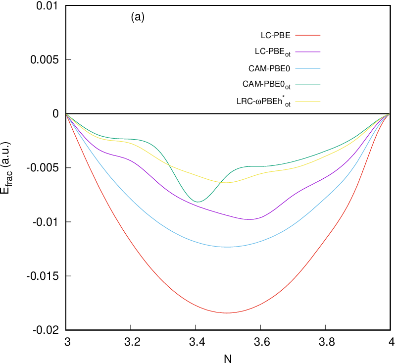
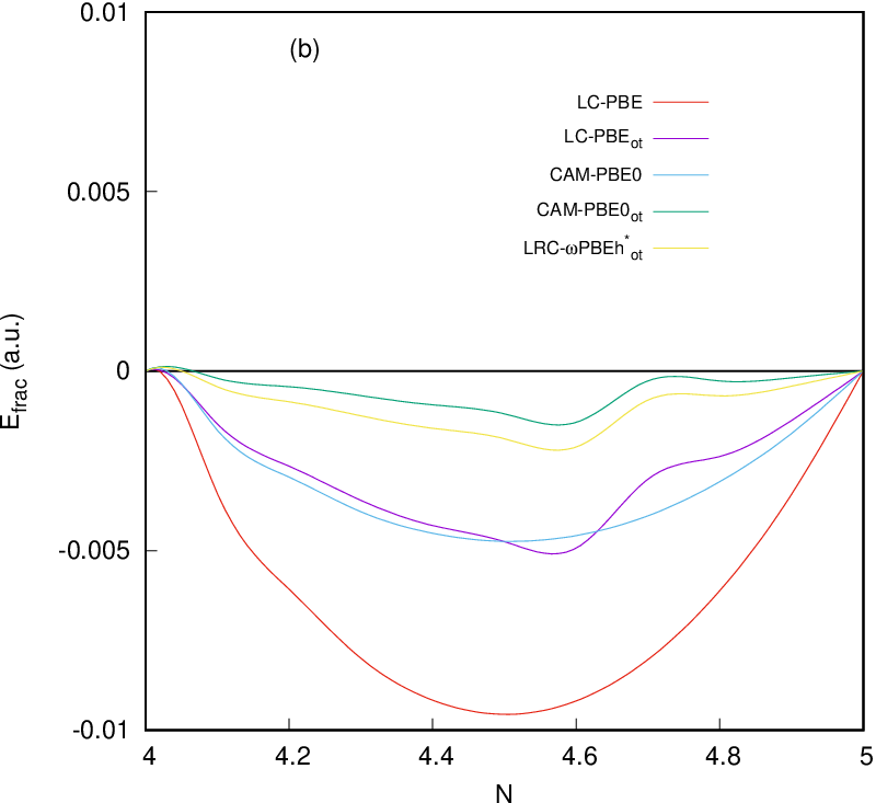
Further, we have also presented the variation of according to Eq. [34] along with Eqs. [29,32]. Once again, C is chosen as a specimen case, to illustrate the relative performance of OT-RSH functionals on PWL behaviour. In an exact scenario, the nature in the range () and () should be straight line. Figure 2 offers this for RSH functionals from PBE0 block; all the five functionals record convex nature, with LC-PBE showing maximum. In keeping with Fig. 1, here also OT-RSH functionals fare better than the conventional RSH. It also appears that, LRC-PBEh and CAM-PBE0 show some similarity between them. These two turn out to be the closest ones near the straight line in region () with much reduced convex deviation. This establishes the fact that the current tuning procedure is sufficient to maintain PWL condition with a considerably small convex deviation.
IV.4 Short polyenes and alkane chains
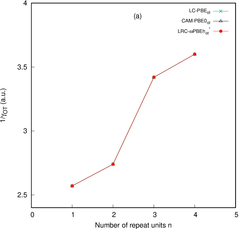
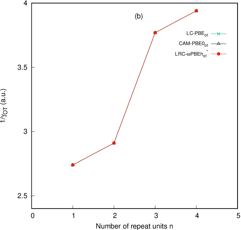
It is known that molecules of similar size can still possess a that is quite different, and the extent of conjugation plays an important role in determining this, besides size (Körzdörfer et al. 2011). To make a direct comparison in such systems, here we pick polyenes, C2nH2n+2, and alkane chains, C2nH4n+2, with , from (Körzdörfer et al. 2011). In this occasion, the repeat unit () is defined in a way such that they are consistent with each other. To pursue this, we plot the characteristic length of SR/LR separation i.e., as defined in (Körzdörfer et al. 2011), as a function of number of repeat unit, in panels (a), (b) of Fig. 3, for polyenes and alkane chains respectively. Only three functionals from PBE0 block are adopted, as the choice of semi-local functionals in determining is completely negligible. From these, a very strong dependence of on chain length is observed, for all three functionals, having identical slope. It is expected, as our self-consistent systematic optimization procedure is based on size dependency principle. To explore the role of conjugation in determining , a comparison between polyenes versus alkane chains is very important, and thus undertaken. It reveals that, the evolution of is linear and similar in both cases. But the value in alkane chains is larger than those for polyenes. Thus, it reaffirms the crucial role played by the extent of conjugation in such a scenario. Therefore, it is consistent with the analysis of (Körzdörfer et al. 2011). A more elaborate comparison for larger may be considered in future; however this basic analysis augurs well for the optimization procedure proposed here.
| PR1 | PR2 | ||||||||||||||
| Atoms | LC-PBE | CAM-PBE | LRC-PBEh | LC-PBE | CAM-PBE | LRC-PBEh | Exp.(Johnson 2016) | ||||||||
| Be | 8.67 | 0.32 | 8.78 | 0.32 | 8.75 | 0.32 | 9.08 | 0.75 | 9.08 | 0.70 | 9.08 | 0.72 | 9.32 | ||
| B | 7.93 | 0.39 | 8.16 | 0.39 | 8.11 | 0.39 | 8.74 | 0.80 | 8.73 | 0.73 | 8.73 | 0.75 | 8.02 | ||
| C | 10.65 | 0.42 | 11.04 | 0.42 | 10.96 | 0.42 | 11.82 | 0.75 | 11.76 | 0.65 | 11.79 | 0.68 | 11.26 | ||
| N | 13.79 | 0.49 | 14.30 | 0.49 | 14.20 | 0.49 | 15.18 | 0.82 | 15.08 | 0.70 | 15.11 | 0.73 | 14.53 | ||
| O | 13.00 | 0.53 | 13.50 | 0.53 | 13.40 | 0.53 | 13.73 | 0.69 | 13.66 | 0.57 | 13.69 | 0.6 | 13.62 | ||
| Si | 8.01 | 0.34 | 8.22 | 0.34 | 8.18 | 0.34 | 8.69 | 0.69 | 8.68 | 0.62 | 8.68 | 0.64 | 8.15 | ||
| P | 10.13 | 0.39 | 10.40 | 0.39 | 10.35 | 0.39 | 10.91 | 0.68 | 10.90 | 0.61 | 10.91 | 0.63 | 10.49 | ||
| S | 10.00 | 0.42 | 10.24 | 0.42 | 10.19 | 0.42 | 9.13 | 0.48 | 9.13 | 0.42 | 9.12 | 0.43 | 10.36 | ||
| Cl | 12.57 | 0.45 | 12.92 | 0.45 | 12.85 | 0.45 | 13.27 | 0.64 | 13.27 | 0.56 | 13.27 | 0.58 | 12.97 | ||
| Ge | 7.62 | 0.34 | 7.79 | 0.34 | 7.76 | 0.34 | 8.20 | 0.68 | 8.19 | 0.62 | 8.19 | 0.63 | 7.90 | ||
| As | 9.57 | 0.36 | 9.82 | 0.36 | 9.77 | 0.36 | 10.31 | 0.66 | 10.30 | 0.59 | 10.31 | 0.61 | 9.82 | ||
| Se | 9.28 | 0.39 | 9.49 | 0.39 | 9.47 | 0.39 | 9.71 | 0.54 | 9.69 | 0.47 | 9.70 | 0.49 | 9.75 | ||
| Br | 11.30 | 0.39 | 11.60 | 0.39 | 11.54 | 0.39 | 11.85 | 0.54 | 11.95 | 0.51 | 11.94 | 0.52 | 11.81 | ||
| MAE | 0.41 | 0.15 | 0.20 | 0.43 | 0.41 | 0.42 | |||||||||
| ME | 0.41 | 0.15 | 0.19 | –0.31 | –0.29 | –0.30 | |||||||||
IV.5 A comparison with traditional optimal tuning
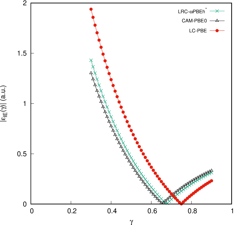
At last, a comparison in the accuracy between present results and conventional OT procedure (Livshits and Baer 2007; Stein et al. 2010; Tamblyn et al. 2014; Kronik et al. 2012), based on Koopmans’ theorem, would be worthwhile. Thus we have examined the IEs of same set of atoms from Table III. In the latter scheme, is tuned in such a way that the HOMO eigenvalue of neutral system equals IE, with the latter determined as a difference in ground-state energy of neutral () and cationic () species. Consequently, the IE-optimized can be obtained by minimizing,
| (36) |
As a specimen case, the implementation of this method is presented in Fig. 4 considering C atom, using three PBE0 block functionals. It is revealed that each plot of vs finds a unique minima for three functionals. This procedure is followed for all atoms, enabling one to estimate the respective ’s. The and its corresponding IE values are presented in Table VII (PR2 columns). As expected, this procedure gives a unique value of for each of them that depends strongly on the electronic structure, and to a lesser extent on the choice of semi-local functionals. The present estimates of along with respective IE’s are provided in PR1 columns. Similar general observations as in PR2, also hold for PR1. It is noticed that is significantly lower in PR1, from PR2.
| PR1 | PR2 | ||||||||||
| Molecules | LC-BLYP | LC-PBE | LC-BLYP | LC-PBE | Exp.(Johnson 2016) | ||||||
| N2 | 14.81 | 0.39 | 14.82 | 0.39 | 16.37 | 0.64 | 16.43 | 0.65 | 15.60 | ||
| Si2 | 7.90 | 0.32 | 8.16 | 0.32 | 7.35 | 0.43 | 8.29 | 0.44 | 7.90 | ||
| P2 | 10.50 | 0.36 | 10.69 | 0.36 | 10.91 | 0.51 | 11.13 | 0.48 | 10.62 | ||
| S2 | 8.69 | 0.36 | 8.86 | 0.36 | 10.13 | 0.52 | 9.48 | 0.51 | 9.40 | ||
| Cl2 | 11.78 | 0.42 | 11.99 | 0.42 | 12.61 | 0.62 | 12.82 | 0.62 | 11.48 | ||
| CO2 | 13.58 | 0.39 | 13.59 | 0.39 | 13.96 | 0.51 | 14.10 | 0.52 | 14.10 | ||
| HCl | 12.35 | 0.49 | 12.54 | 0.49 | 12.90 | 0.58 | 13.06 | 0.57 | 12.79 | ||
| CO | 13.58 | 0.39 | 13.59 | 0.39 | 14.28 | 0.50 | 14.24 | 0.49 | 14.10 | ||
| H2O | 11.51 | 0.39 | 11.55 | 0.39 | 12.59 | 0.55 | 12.64 | 0.55 | 12.62 | ||
| H2S | 10.11 | 0.39 | 10.29 | 0.39 | 10.60 | 0.51 | 10.71 | 0.49 | 10.48 | ||
| C2H2 | 11.04 | 0.39 | 11.24 | 0.39 | 11.32 | 0.46 | 11.49 | 0.45 | 11.40 | ||
| NH3 | 9.86 | 0.39 | 9.96 | 0.39 | 10.48 | 0.49 | 10.58 | 0.49 | 10.82 | ||
| PH3 | 9.96 | 0.36 | 10.10 | 0.36 | 10.36 | 0.46 | 10.43 | 0.44 | 9.89 | ||
| CH4 | 13.78 | 0.42 | 13.91 | 0.42 | 14.17 | 0.49 | 14.29 | 0.49 | 13.60 | ||
| CH3Cl | 11.04 | 0.39 | 11.20 | 0.39 | 11.39 | 0.46 | 11.55 | 0.46 | 11.29 | ||
| C2H4 | 10.18 | 0.36 | 10.41 | 0.36 | 10.39 | 0.42 | 10.56 | 0.40 | 10.51 | ||
| C2H6 | 11.95 | 0.36 | 12.06 | 0.36 | 12.49 | 0.46 | 12.60 | 0.46 | 11.99 | ||
| SiH4 | 12.37 | 0.34 | 12.49 | 0.34 | 12.96 | 0.46 | 13.12 | 0.47 | 12.30 | ||
| Si2H6 | 10.59 | 0.32 | 10.75 | 0.32 | 10.81 | 0.37 | 10.93 | 0.36 | 10.53 | ||
| MAE | 0.38 | 0.36 | 0.32 | 0.40 | |||||||
| ME | 0.31 | 0.17 | –0.19 | –0.37 | |||||||
Let us now discuss the accuracy of these two methods, in terms of MAE and ME values collected at the bottom of the table. A glance reveals that, for all three functionals, these are identical in PR1, with all ME having ()ve sign. In contrast, the ME values are found to be ()ve for all functionals in case of conventional PR2 scheme. This indicates an underestimation and overestimation of IE from experiment, in PR1 and PR2 respectively. However, these error are systematic in nature. Now, the performance of these methods is reflected through respective MAE values. Though the MAE of LC-PBE in PR1 is very close to that of PR2, but the same in case of remaining two functionals is substantially lower (at least by a factor of 2) in PR1 from their PR2 counterparts, implying PR1 to be supposedly more accurate than PR2.
Next, we also consider the IEs of same set of molecules from Table IV (excluding NaCl) using present and conventional OT procedure as presented in Table VII, for atoms. It is already mentioned that the auxiliary parameters () used in different functionals may have some sensitivity during self-consistent tuning process, and it is indeed important for molecular systems. To be consistent with this fact, here, two such functionals such as LC-BLYP and LC-PBE, which are devoid of auxiliary parameters, are used for an unbiased comparison. In the conventional OT scheme, we follow the same procedure as depicted in Fig. 4 for all molecules. The and its corresponding IE values are presented in Table VIII (PR2 columns). As in atoms, this procedure gives a unique value of for each of them that depends strongly on the electronic structure, and to a lesser extent on the choice of semi-local functionals. The present estimates of along with respective IE’s are provided in PR1 columns. Similar general observations as in PR2, also hold for PR1. Further, we also found the same trend in ; which is usually lower in PR1, compared with PR2.
A glance at MAE and ME at the bottom of the table reveals that, for two such functionals, these are quite close for PR1 and PR2 having ()ve and ()ve signs in MEs. This indicates an underestimation and overestimation of IE from experiment, in PR1 and PR2 respectively. However, these error are not systematic as found in case of atoms. Moreover, the MAE values signify that these two methods are reasonably close to each other in terms of accuracy. It is to be noted that values differ significantly (for the same system and functional) from the IP-tuning approach, which was also observed in case of atoms. But, it is consistent with the fact that if we follow carefully the ME values which are (+) and (-) signs for the present method and IP-tuning approach respectively.
A few remarks may now be made before passing. The computational overhead of each step during optimization is at same level as in commonly used standard RSH functionals; the additional time is required only for grid optimization as discussed in Tables I, II. The computation cost for each optimization step with respect to system size has already been mentioned in Sec. II(B), and hence not repeated here. Moreover, if we consider to be the time required to complete one SCF cycle, the number of SCF iteration and as total number of optimization steps, then the real time computational cost can be simply estimated as: . This equivalently holds for PR2 method. However, a real time difference can only come through the respective value of and . Now the basic advantage of our method is its ease of implementation through a simple energy optimization, keeping the development from first principles and this may offer considerable benefit for periodic systems, for which calculation on charged systems can be rather difficult. Moreover, it is sufficient to maintain Koopmans’ theorem (Salzner and Baer 2009) and PWL conditions without imposing it during optimization. In future, it may be a viable alternative to popular ab initio OT-RSH schemes (Livshits and Baer 2007; Stein et al. 2010; Tamblyn et al. 2014; Kronik et al. 2012). It would be worthwhile to compare our results with the latter scheme in terms of accuracy and cost in a more elaborate fashion for other properties besides IE. Currently this is being pursued and may be communicated in future.
V Future and Outlook
We have demonstrated the feasibility and practicability of a self-consistent systematic optimization procedure for OT-RSH functionals from first principles. This was applied for a host of atoms and molecules; properties derived from frontier orbital energies were offered, within a pseudopotential (G)KS-DFT framework. Besides these, their performances on fractional occupation of electron on HOMO were also presented. The accuracy of OT-RSH functionals is always improved than that of RSH functionals for all the species in case of both B3LYP and PBE0 series, in case of the properties derived from orbital energies. The success of this approach relies on accurate estimation of based on size dependency principle.
So far, we have taken in to account only the properties derived from frontier orbital energies. But, other properties derived from total energy of a system, may also improve the quality of these designed functionals. In this scenario, an extensive analysis is required to maintain the size consistency on total energy. Again, the compatibility of with auxiliary parameters present in RSH functionals should be taken into consideration during the optimization procedure. Furthermore, the relative performance of B3LYP block functionals seems to be less affected by our proposed scheme. This leads us to conclude that, there is a possibility of further improving the results, notably, by incorporating the recently developed SR GGA exchange functionals satisfying a set of prescribed constraints, and using better basis set from all-electron calculations. In essence, we believe that the current approach may provide a useful practical framework for future development and application (such as static electric response properties, charge-transfer excitation, Rydberg excitation).
VI Availability of data
Data available on request from the authors.
VII Acknowledgement
AG is grateful to UGC for a senior research fellowship. AKR thankfully acknowledges funding from DST SERB, New Delhi, India (sanction order: CRG/2019/000293).
References
- Hohenberg and Kohn (1964) P. Hohenberg and W. Kohn, Phys. Rev. 136, B864 (1964).
- Cohen et al. (2011) A. J. Cohen, P. Mori-Sánchez, and W. Yang, Chem. Rev. 112, 289 (2011).
- Burke (2012) K. Burke, J. Chem. Phys. 136, 150901 (2012).
- Becke (2014) A. D. Becke, J. Chem. Phys. 140, 18A301 (2014).
- Jones (2015) R. O. Jones, Rev. Mod. Phys. 87, 897 (2015).
- Kohn and Sham (1965) W. Kohn and L. J. Sham, Phys. Rev. 140, A1133 (1965).
- Seidl et al. (1996) A. Seidl, A. Görling, P. Vogl, J. A. Majewski, and M. Levy, Phys. Rev. B 53, 3764 (1996).
- Becke (1988) A. D. Becke, Phys. Rev. A 38, 3098 (1988).
- Perdew et al. (1996a) J. P. Perdew, K. Burke, and M. Ernzerhof, Phys. Rev. Lett. 77, 3865 (1996a).
- Tao et al. (2003) J. Tao, J. P. Perdew, V. N. Staroverov, and G. E. Scuseria, Phys. Rev. Lett. 91, 146401 (2003).
- Zhao and Truhlar (2008) Y. Zhao and D. G. Truhlar, Theor. Chem. Acc. 41, 157 (2008).
- Perdew and Schmidt (2000) J. P. Perdew and K. Schmidt, AIP Conf. Proc. 577, 1 (2000).
- Becke (1993) A. D. Becke, J. Chem. Phys. 98, 1372 (1993).
- Perdew et al. (1996b) J. P. Perdew, M. Ernzerhof, and K. Burke, J. Chem. Phys. 105, 9982 (1996b).
- Becke (2005) A. D. Becke, J. Chem. Phys. 122, 064101 (2005).
- Perdew et al. (2008) J. P. Perdew, V. N. Staroverov, J. Tao, and G. E. Scuseria, Phys. Rev. A 78, 052513 (2008).
- Grimme and Neese (2007) S. Grimme and F. Neese, J. Chem. Phys. 127, 154116 (2007).
- Zhang et al. (2009) Y. Zhang, X. Xu, and W. Goodard, Proc. Nat. Acad. Sci. (USA). 106, 4963 (2009).
- Perdew and Wang (1992) J. P. Perdew and Y. Wang, Phys. Rev. B 45, 13244 (1992).
- Yang et al. (2000) W. Yang, Y. Zhang, and P. W. Ayers, Phys. Rev. Lett. 84, 5172 (2000).
- Perdew and Zunger (1981) J. P. Perdew and A. Zunger, Phys. Rev. B 23, 5048 (1981).
- Bao et al. (2018) J. L. Bao, L. Gagliardi, and D. G. Truhlar, J. Phys. Chem. Lett. 9, 2353 (2018).
- Levy et al. (1984) M. Levy, J. P. Perdew, and V. Sahni, Phys. Rev. A 30, 2745 (1984).
- Kronik and Kümmel (2020) L. Kronik and S. Kümmel, Phys. Chem. Chem. Phys. 22, 16467 (2020).
- Kronik and Kümmel (2018) L. Kronik and S. Kümmel, Adv. Mat. 30, 1706560 (2018).
- Baer et al. (2010) R. Baer, E. Livshits, and U. Salzner, Annu. Rev. Phys. Chem. 61, 85 (2010).
- Leininger et al. (1997) T. Leininger, H. Stoll, H. J. Werner, and A. Savin, Chem. Phys. Lett. 275, 151 (1997).
- Iikura et al. (2001) H. Iikura, T. Tsuneda, and K. Hirao, J. Chem. Phys. 115, 3540 (2001).
- Tawada et al. (2004) Y. Tawada, T. Tsuneda, S. Yanagisawa, T. Yanai, and K. Hirao, J. Chem. Phys. 120, 8425 (2004).
- Yanai et al. (2004) T. Yanai, D. P. Tew, and N. C. Handy, Chem. Phys. Lett. 393, 51 (2004).
- Lange et al. (2008) A. W. Lange, M. A. Rohrdanz, and J. M. Herbert, J. Phys. Chem. B 112, 6304 (2008).
- Salzner and Baer (2009) U. Salzner and R. Baer, J. Chem. Phys. 131, 231101 (2009).
- Livshits and Baer (2007) E. Livshits and R. Baer, Phys. Chem. Chem. Phys. 9, 2932 (2007).
- Stein et al. (2010) T. Stein, H. Eisenberg, L. Kronik, and R. Baer, Phys. Rev. Lett. 105, 266802 (2010).
- Borpuzari and Kar (2017) M. P. Borpuzari and R. Kar, J. Comput. Chem. 38, 2258 (2017).
- Wang and Zhang (2018) C. Wang and Q. Zhang, J. Phys. Chem. C 123, 4407 (2018).
- Tamblyn et al. (2014) I. Tamblyn, S. Refaely-Abramson, J. B. Neaton, and L. Kronik, J. Phys. Chem. Lett. 5, 2734 (2014).
- Ghosal et al. (2019) A. Ghosal, T. Mandal, and A. K. Roy, J. Chem. Phys. 150, 064104 (2019).
- Ghosal and Roy (2016) A. Ghosal and A. K. Roy, In Specialist Periodical Reports: Chemical Modelling, Applications and Theory; M. Springborg and J.-O. Joswig (Eds.) Vol. 13 (Royal Society of Chemistry, London, 2016).
- Ghosal et al. (2018) A. Ghosal, T. Mandal, and A. K. Roy, Int. J. Quant. Chem. 118, e25708 (2018).
- Roy (2008a) A. K. Roy, Int. J. Quant. Chem. 108, 837 (2008a).
- Roy (2008b) A. K. Roy, Chem. Phys. Lett. 461, 142 (2008b).
- Roy (2010) A. K. Roy, Trends in Phys. Chem. 14, 27 (2010).
- Roy (2011) A. K. Roy, J. Math. Chem. 49, 1687 (2011).
- Roy (2009) A. K. Roy, in Handbook of Computational Chemistry Research, edited by C. T. Collett and C. D. Robson (Nova publishers, New York, 2009), pp. 409–434.
- Obara and Saika (1986) S. Obara and A. Saika, J. Chem. Phys. 84, 3963 (1986).
- Obara and Saika (1988) S. Obara and A. Saika, J. Chem. Phys. 89, 1540 (1988).
- Head-Gordon and Pople (1988) M. Head-Gordon and J. A. Pople, J. Chem. Phys. 89, 5777 (1988).
- Liu et al. (2016) F. Liu, T. Furlani, and J. Kong, J. Phys. Chem. A 120, 10264 (2016).
- Baer and Neuhauser (2005) R. Baer and D. Neuhauser, Phys. Rev. Lett. 94, 043002 (2005).
- Mandal et al. (2019) T. Mandal, A. Ghosal, and A. K. Roy, Theor. Chem. Acc. 138, 10 (2019).
- Körzdörfer et al. (2011) T. Körzdörfer, J. S. Sears, C. Sutton, and J.-L. Brédas, J. Chem. Phys. 135, 204107 (2011).
- Martyna and Tuckerman (1999) G. J. Martyna and M. E. Tuckerman, J. Chem. Phys. 110, 2810 (1999).
- Kronik et al. (2012) L. Kronik, T. Stein, S. Refaely-Abramson, and R. Baer, J. Chem. Theory Comput. 8, 1515 (2012).
- Rohrdanz et al. (2009) M. A. Rohrdanz, K. M. Martins, and J. M. Herbert, J. Chem. Phys. 130, 054112 (2009).
- Chai and Head-Gordon (2008a) J.-D. Chai and M. Head-Gordon, Chem. Phys. Lett. 467, 176 (2008a).
- Chai and Head-Gordon (2008b) J.-D. Chai and M. Head-Gordon, J. Chem. Phys. 128, 084106 (2008b).
- Peverati and Truhlar (2012) R. Peverati and D. G. Truhlar, Phys. Chem. Chem,. Phys. 14, 16187 (2012).
- Vikramaditya et al. (2018) T. Vikramaditya, J.-D. Chai, and S.-T. Lin, J. Comp. Chem. 39, 2378 (2018).
- Chan et al. (2019) B. Chan, Y. Kawashima, and K. Hirao, J. Comput. Chem. 40, 29 (2019).
- Henderson et al. (2008) T. M. Henderson, B. G. Janesko, and G. Scuseria, J. Chem. Phys. 128, 194105 (2008).
- Cohen et al. (2007) A. J. Cohen, P. Mori-Sánchez, and W. Yang, J. Chem. Phys. 126, 191109 (2007).
- Lin et al. (2012) Y.-S. Lin, C.-W. Tsai, G.-D. Li, and J.-D. Chai, J. Chem. Phys. 136, 154109 (2012).
- Johnson et al. (1993) B. G. Johnson, P. M. W. Gill, and J. A. Pople, J. Chem. Phys. 98, 5612 (1993).
- Ernzerhof and Perdew (1998) M. Ernzerhof and J. P. Perdew, J. Chem. Phys. 109, 3313 (1998).
- A. K. Roy, A. Ghosal and T. Mandal (2019) A. K. Roy, A. Ghosal and T. Mandal, InDFT: A DFT Program for Atoms and Molecules in CCG (Theoretical Chemistry Laboratory, IISER Kolkata, India, 2019), This is based on the extension of an initial version of the code, established by A. K. Roy, in 2008, whose results were published in refs. [41-45].
- Stephens et al. (1994) P. J. Stephens, F. J. Devlin, C. F. Chabalowski, and M. J. Frisch, J. Chem. Phys. 98, 11623 (1994).
- Schmidt et al. (1993) M. W. Schmidt, K. K. Baldridge, J. A. Boatz, S. T. Elbert, M. S. Gordon, J. H. Hensen, S. Koseki, N. Matsunaga, K. A. Nguyen, S. J. Su, et al., J. Comput. Chem. 14, 1347 (1993).
- Stevens et al. (1984) W. J. Stevens, H. Basch, and M. Krauss, J. Chem. Phys. 81, 6026 (1984).
- Hay and Wadt (1985) P. J. Hay and W. R. Wadt, J. Chem. Phys. 82, 284 (1985).
- Feller (1996) D. Feller, J. Comp. Chem. 17, 1571 (1996).
- Vosko et al. (1980) S. H. Vosko, L. Wilk, and M. Nusair, Can. J. Phys. 58, 1200 (1980).
- Lee et al. (1988) C. Lee, W. Yang, and R. G. Parr, Phys. Rev. B 37, 785 (1988).
- rep (2001) Density Functional Repository, Quantum Chemistry Group (CCLRC Daresbury Laboratory, Daresbury, Cheshire, UK, 2001).
- Frigo and Johnson (2005) M. Frigo and S. G. Johnson, Proceedings of the IEEE 93, 216 (2005).
- Anderson et al. (1999) E. Anderson, Z. Bai, C. Bischof, S. Blackford, J. Dongarra, J. D. C. A. Greenbaum, S. Hammarling, A. A. McKenney, and D. Sorensen, LAPACK Users’ Guide, vol. 9 (SIAM, 1999).
- Johnson (2016) R. D. Johnson, III (Ed.) NIST Computational Chemistry Comparisons and Benchmark Database, NIST Standard Reference Database, Number, Release 18 (NIST, Gaithersburg, MD, 2016).
- Ghosal et al. (2021) A. Ghosal, T. Gupta, K. Mahato, and A. K. Roy, Theor. Chem. Acc. 140, 1 (2021).
- Perdew et al. (1982) J. P. Perdew, R. G. Parr, M. Levy, and J. L. Balduz Jr., Phys. Rev. Lett. 49, 1691 (1982).
- Perdew and Levy (1997) J. P. Perdew and M. Levy, Phys. Rev. B 56, 16021 (1997).
- Görling and Levy (1997) A. Görling and M. Levy, J. Chem. Phys. 106, 2675 (1997).
- Pople et al. (1989) J. A. Pople, M. Head-Gordon, D. J. Fox, K. Raghavachari, and L. A. Curtiss, J. Chem. Phys. 90, 5622 (1989).
- Landau (1957) L. D. Landau, Sov. Phys. JETP 3, 920 (1957).
- Mori-Sánchez et al. (2006) P. Mori-Sánchez, A. J. Cohen, and W. Yang, J. Chem. Phys. 124, 091102 (2006).
- Janak (1978) J. F. Janak, Phys. Rev. B 18, 7165 (1978).