Robust Quantity-Aware Aggregation for Federated LearningDOI: XXXXXXX.XXXXXXXConference: 29th ACM SIGKDD Conference on Knowledge Discovery and Data Mining; August 6-10, 2023; Long Beach, CA, USAPrice: 15.00ISBN: 978-1-4503-XXXX-X/18/06CCS: Security and privacy Privacy protectionsCCS: Computing methodologies Cooperation and coordinationCCS: Computing methodologies Distributed artificial intelligence
Abstract.
Federated Learning (FL) enables multiple clients to collaborate on training machine learning models without sharing their data, making it an important privacy-preserving framework. However, FL is susceptible to security and robustness challenges, such as malicious clients potentially corrupting model updates and amplifying their impact through excessive quantities. Existing defenses for FL, while all handling malicious model updates, either treat all quantities as benign or ignore/truncate quantities from all clients. The former is vulnerable to quantity-enhanced attacks, while the latter results in sub-optimal performance due to the varying sizes of local data across clients. In this paper, we introduce a robust quantity-aware aggregation algorithm for FL called FedRA. FedRA considers local data quantities during aggregation and defends against quantity-enhanced attacks. It consists of two crucial components, i.e., a quantity-robust scorer and a malicious client number estimator. More specifically, the quantity-robust scorer calculates the sum of the distance between one update and the rest of the updates as the quantity-robust score, taking into account their quantities as factors. The malicious client number estimator uses these scores to predict the number of suspicious clients to exclude in each round, adapting to the dynamic number of malicious clients participating in FL in each round. Experiments on three public datasets demonstrate FedRA’s effectiveness in defending against quantity-enhanced attacks in FL. The code for FedRA can be found at https://anonymous.4open.science/r/FedRA-4C1E.
Abstract.
Federated Learning (FL) enables multiple clients to collaborate on training machine learning models without sharing their data, making it an important privacy-preserving framework. However, FL is susceptible to security and robustness challenges, such as malicious clients potentially corrupting model updates and amplifying their impact through excessive quantities. Existing defenses for FL, while all handling malicious model updates, either treat all quantities as benign or ignore/truncate quantities from all clients. The former is vulnerable to quantity-enhanced attacks, while the latter results in sub-optimal performance due to the varying sizes of local data across clients. In this paper, we introduce a robust quantity-aware aggregation algorithm for FL called FedRA. FedRA considers local data quantities during aggregation and defends against quantity-enhanced attacks. It consists of two crucial components, i.e., a quantity-robust scorer and a malicious client number estimator. More specifically, the quantity-robust scorer calculates the sum of the distance between one update and the rest of the updates as the quantity-robust score, taking into account their quantities as factors. The malicious client number estimator uses these scores to predict the number of suspicious clients to exclude in each round, adapting to the dynamic number of malicious clients participating in FL in each round. Experiments on three public datasets demonstrate FedRA’s effectiveness in defending against quantity-enhanced attacks in FL. The code for FedRA can be found at https://anonymous.4open.science/r/FedRA-4C1E.
Keywords:
robustness, federated learning, quantity1. Introduction
Federated learning (FL) is an important technology to train models while protecting the privacy of training data. It has been extensively studied for various application scenarios, such as medical health (Rieke et al. 2020; Sheller et al. 2020; Xu et al. 2021; Nguyen et al. 2022; Kumar and Singla 2021) and keyboard next-word prediction (Yang et al. 2018; Hard et al. 2018; Chen et al. 2019; Li et al. 2020a; Ramaswamy et al. 2019). One of the classic FL algorithms is FedAvg (McMahan et al. 2017). In FedAvg, the server iteratively averages clients’ updates with some weights determined by the quantity of each client, which means throughout the paper the number of the training data at that client, to update the global model.
The linear aggregation used in FedAvg has been shown to be vulnerable to poisoning attacks (Baruch et al. 2019; Fang et al. 2020; Wang et al. 2020; Liu et al. 2017; Bagdasaryan et al. 2020; Bhagoji et al. 2019; Xie et al. 2021). These attacks primarily aim to either deteriorate the performance of the global model or insert a backdoor into the global model. However, malicious clients can also submit large quantities to obtain unfairly high weights in the model aggregation, leading to a heightened impact of their malicious updates on the global model. We refer to this type of attack as quantity-enhanced attacks.
Several methods have been proposed to defend against poisoning attacks for federated learning (Blanchard et al. 2017; Yin et al. 2018; El Mhamdi et al. 2018; Sun et al. 2019; Pillutla et al. 2019; Portnoy et al. 2020). These defenses can be categorized into three groups: quantity-ignorant, quantity-aware, and quantity-robust defenses. Quantity-ignorant defenses aggregate updates without considering quantities (Blanchard et al. 2017; Yin et al. 2018; El Mhamdi et al. 2018). These methods are robust to quantity-enhanced attacks. However, since aggregating updates with quantities benefits model performance (Zaheer et al. 2018; Reddi et al. 2021), applying these defenses may lead to performance degradation. Quantity-aware defenses aggregate updates with quantities but by default treat quantities submitted by clients as benign (Sun et al. 2019; Pillutla et al. 2019). These defenses outperform quantity-ignorant defenses when there are no attacks, but their performance deteriorates significantly when faced with quantity-enhanced attacks. Quantity-robust defenses aggregate updates with quantities and, unlike quantity-aware defenses, are robust to quantity-enhanced attacks. Portnoy et al. 2020 propose to truncate quantities with a dynamic threshold and apply quantity-aware Trimean (Yin et al. 2018) to aggregate updates. However, it handles updates and quantities separately, which could result in the truncation of the quantities of benign clients, ultimately leading to sub-optimal performance.
Meanwhile, some existing defenses (Blanchard et al. 2017; Yin et al. 2018; El Mhamdi et al. 2018) need a parameter that represents the upper bound of the number of malicious clients to be filtered out in each round. However, in cross-device federated learning, due to the large number of clients, only a subset of clients is selected for participation in each round. As a result, the number of malicious clients in each round changes dynamically. Over-estimating the number of malicious clients leads to some benign clients being filtered out, while underestimating the number of malicious clients may result in some malicious updates being included in the model aggregation.
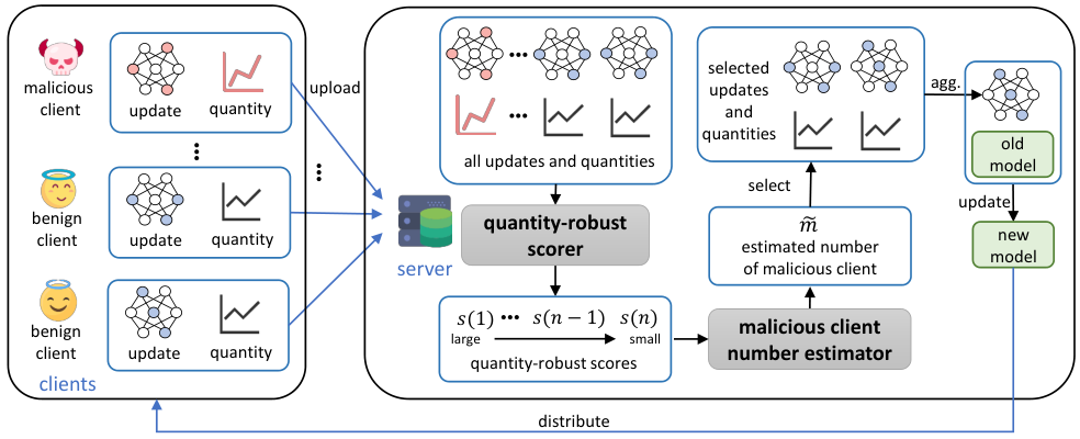
In this paper, we propose FedRA, a quantity-robust defense for federated learning. It filters out malicious clients by taking both quantities and updates into consideration. More specifically, FedRA consists of two components, i.e., quantity-robust scorer and malicious client number estimator. The quantity-robust scorer is based on the observation that the expectation of distance between benign updates with larger quantities should be smaller. Therefore, to compute the quantity-robust score, we calculate the sum of distances between one update and the rest of the updates, taking into account the quantities as coefficients. The coefficient is smaller when the pair of quantities are larger. The malicious client number estimator uses the quantity-robust scores as input and predicts the number of malicious clients to exclude in each round by maximizing the log-likelihood. Finally, the corresponding number of updates with the largest quantity-robust scores are filtered out. The rest updates are aggregated with weights proportional to their quantities to update the global model.
The main contributions of this paper are as follows:
- •
We propose a robust quantity-aware aggregation method for federated learning to aggregate updates with quantities while defending against quantity-enhanced attacks.
- •
We theoretically prove FedRA is quantity-robust by proving its aggregation error is irrelevant to malicious quantities.
- •
We conduct experiments on three public datasets to validate the effectiveness of FedRA.
2. Related Works
2.1. Federated Learning
Federated learning (McMahan et al. 2017) enables multiple clients collaboratively train models without sharing their local datasets. There are three steps in each round of federated learning. First, a central server randomly samples a group of clients and distributes the global model to them. Second, the selected clients train the model with their local datasets and upload their model updates to the central server. Finally, the central server aggregates the received updates to update the global model. In FedAvg (McMahan et al. 2017), updates are weight-averaged according to the quantity of each client’s training samples. Reddi et al. 2021 have proposed FedAdam, where the server updates the global model with Adam optimizer. The above steps are performed iteratively until the global model converges.
2.2. Federated Poisoning Attacks
However, classical federated learning is vulnerable to poisoning attacks, e.g., untargeted attacks (Baruch et al. 2019; Fang et al. 2020) and backdoor attacks (Liu et al. 2017; Bagdasaryan et al. 2020; Wang et al. 2020; Xie et al. 2020; Bhagoji et al. 2019). In this paper, we focus on defending against untargeted attacks, which aim to degrade the performance of the global model on arbitrary input samples. Label flip (Fang et al. 2020) is a data-poisoning-based untargeted attack, where the malicious clients manipulate the labels of their local training dataset to generate malicious updates. Some advanced attacks assume the malicious clients have knowledge of benign datasets and can collaborate to generate malicious updates. LIE (Baruch et al. 2019) adds small noises to the average of benign updates to circumvent defenses. Optimize (Fang et al. 2020) models the attack as an optimization problem and adds noises in the opposite direction of benign updates. These attacks focus on generating malicious updates, but overlook the attacker can submit large quantities to obtain unfairly high weight in model aggregation.
2.3. Robust Aggregations
To defend against untargeted attacks in federated learning, several robust aggregation methods have been proposed. Yin et al. 2018 propose Median and Trimean that apply coordinate-wise median and trimmed-mean, respectively, to filter out malicious updates. Blanchard et al. 2017 propose Krum and mKrum that compute square-distance-based scores to select and average the updates closest to a subset of neighboring updates. Bulyan (El Mhamdi et al. 2018) is a combination of mKrum and Trimean: it first selects several updates through mKrum and then aggregates them with Trimean. We note that the above defense methods do not consider quantities of clients’ training samples, which we categorize as quantity-ignorant methods, and the convergence speeds and model performance of these methods are compromised (Zaheer et al. 2018; Reddi et al. 2021), especially for quantity-imbalanced scenarios, such as long-tailed data distributions that are common in real-world scenarios (Zhang et al. 2017; Zhong et al. 2019; Li et al. 2017).
Sun et al. 2019 propose Norm-bound that clips the norm of received updates to a predefined threshold. Pillutla et al. 2019 propose RFA that computes weights for each update by running an approximation algorithm to minimize the quantity-aware geometric median of updates. These two methods are categorized into quantity-aware defenses. They take quantities into consideration when aggregating updates but by default treat all received quantities as benign. Portnoy et al. 2020 point out that received quantities may be malicious and can be exploited to increase the impact of malicious updates. They further propose a Truncate method that truncates received quantities within a dynamic threshold in each round, which guarantees any 10% clients do not have more than 50% samples. The Truncate method is categorized into quantity-robust method. However, quantities of benign clients with a large number of training samples may also be truncated, resulting in degraded performance. Meanwhile, they handle the malicious update filtering and the quantity truncation separately, which is sub-optimal.
3. Problem Definition
Suppose that training samples are sampled from a distribution in sample space . Let denote the loss function of model parameter at data point , and is the corresponding population loss function. The goal is to minimize the population loss by training the model parameter, i.e., .
Assume that there are clients in total and of them are malicious. The -th client has a local dataset . The empirical loss of the -th client is . In the -th round, the central server randomly samples clients and distributes the global model to them. Following existing works (Yin et al. 2018; Blanchard et al. 2017; El Mhamdi et al. 2018), we define a benign client will submit update and quantity , while a malicious client can submit an arbitrary update and an arbitrary quantity to the server. After receiving the updates and quantities from the sampled clients, the server computes the global update with a certain aggregation rule : .
Some existing robust aggregation algorithms, e.g., mKrum (Blanchard et al. 2017), Bulyan (El Mhamdi et al. 2018), and Trimean (Yin et al. 2018), require estimation of the upper bound of the number of malicious clients, denoted by , in each round using a fixed parameter for all rounds. However, in cross-device federated learning, due to the large number of clients, only a subset of clients is selected for participation in each round. The number of malicious clients in each round follows a hypergeometric distribution and is thus hard to be estimated by a fixed parameter. Over-estimating the number of malicious clients leads to some benign clients being filtered out, while underestimating the number of malicious clients may result in some malicious updates being included in the model aggregation. In our work, we consider two settings: fixed-ratio setting and dynamic-ratio setting. In the fixed-ratio setting, the number of malicious clients in each round is fixed, i.e., . Since is not a random variable, estimating with a fixed parameter is feasible. The fixed-ratio setting, while not representative of real-world cross-device federated learning, provides a baseline for the upper limit of defense performance in filtering out malicious updates. In contrast, the dynamic-ratio setting involves a fixed total number of malicious clients, , but the exact number of malicious clients per round is unknown, which better reflects real-world federated learning situations.
4. Threat Model
Following existing works (Fang et al. 2020), in this section, we introduce the objective, knowledge, and capability of attackers and the details of quantity-enhanced attacks.
Attacker’s Objective. The attacker’s objective is to carry out untargeted attacks on the federated learning system, which aims to degrade the overall performance of the global model on arbitrary input samples.
Attacker’s Knowledge. Since the server distributes the global model to clients in each round, the attacker knows the model structure, the local model parameters, and the local training code. Due to the privacy-protecting nature of federal learning, the attacker cannot access the datasets of other clients. Thus, the attacker has partial knowledge of the data distribution. Since the server might not release its aggregation code, the attacker does not know the aggregation rule applied by the server.
Attacker’s Capability. Building on prior attack methods (Baruch et al. 2019; Fang et al. 2020), we consider the scenario where an attacker controls malicious clients. These clients can coordinate with each other and use benign data stored on their devices to generate malicious updates and quantities. If any of the malicious clients are selected by the server, they can upload the malicious updates and quantities to the server, degrading the performance of the global model.
Quantity-enhanced Attack. In addition to generating malicious updates via existing untargeted attacks, the attacker also submits large quantities to obtain unfairly high weight in model aggregation, resulting in an amplified impact of malicious updates on the global model. The malicious clients first collaborate to compute the mean and standard deviation of their quantities, which are denoted as and , respectively. The final submitted quantity is defined as , where is the quantity-enlarging factor. should be as large as possible but not detectable by the server
5. Existing Defenses Are Sub-optimal in Quantity-imbalanced Scenarios
In this section, we prove that both quantity-ignorant and quantity-aware defenses are sub-optimal in quantity-imbalanced scenarios. To simulate quantity-imbalanced settings, we make the quantities of the benign client datasets obey log-normal distributions, which is a typical common long-tailed distribution in real-world scenarios (Li et al. 2019; Park and Tuzhilin 2008; Chen et al. 2020; Kim et al. 2019; Long et al. 2022). The detailed experimental settings are in Section 8.
5.1. Quantity-ignorant Methods
In this subsection, we compare the performance of quantity-ignorant methods (Krum, mKrum, Median, TriMean, Bulyan, and Uniform) with that of quantity-aware methods (FedAdam, Norm-bounding, and RFA) in both IID and non-IID non-attack settings. The experimental results on MNIST, CIFAR10, and MIND are shown in Figure 1. We can observe that the performance of quantity-ignorant methods is consistently lower than that of quantity-aware methods. This is because the expectation of the local model error decreases as the sample size of the training dataset increases (Ruder 2016). Assigning higher weight to the local models trained with larger datasets reduced the aggregation error of the global model.
5.2. Quantity-aware Methods
In this subsection, we analyze the performance of quantity-aware methods (FedAdam, Norm-bounding, and RFA) in IID fixed-ratio settings when exposed to quantity-enhanced attacks. We set the quantity-enlarging factor . Due to the space limitation, we show the results of LIE-based quantity-enhanced attacks on MNIST datasets in Figure 2. We can observe that the performance of quantity-aware methods degrades as the quantity-enlarging factor increases. This is because these methods by default treat the quantities submitted by clients as benign, which is vulnerable to quantity-enhanced attacks since the large quantities can amplify the impact of malicious updates.
We also show the performance of Truncate in Figure 2. We can observe that its performance is stable but sub-optimal under the quantity-enhanced attack. This is because although Truncate limits the upper bound of malicious quantities, it also clips the quantities of benign clients. Additionally, the separate handling of malicious quantities and updates restricts Truncate’s ability to effectively filter malicious updates.
6. Methodology
In this section, we introduce the details of our robust quantity-aware aggregation, named FedRA, which aims to be quantity-robust and achieve optimal performance. It contains two core components, i.e. a quantity-robust scorer and a malicious client number estimator. The quantity-robust scorer calculates scores for clients based on their uploaded updates and quantities. The malicious client number estimator dynamically determines the number of malicious clients in each round, which is more suitable for the dynamic-ratio setting. The framework of our FedRA is shown in Figure 3.
6.1. Quantity-robust Scorer
Lemma 0.
Lemma 1 is proved in Appendix A.3, which reflects that the distance between two benign updates varies according to their quantities. If the quantities of two clients are larger, the distance between their updates should be smaller. Inspired by this observation, we design a quantity-robust score, which aims to filter malicious clients considering both their updates and quantities. The quantity-robust score of the -th client is defined as follows
| (2) |
where denotes that belongs to the updates closest to in terms of the value, is the estimated number of malicious client, is a hyper-parameter. A smaller quantity-robust score indicates the client is more likely to be benign.
6.2. Malicious Client Number Estimator
Then we need to determine the number of clients to select in each round, which is denoted as . In the fixed-ratio setting, we can set , where is the estimated number of malicious clients in each round and is the estimated number of overall malicious clients. However, in the dynamic-ratio setting, the number of malicious clients varies in each round. Over-estimating may result in filtering some benign clients, while underestimating may include some malicious updates in the model aggregation. Therefore, we propose a malicious client number estimator to predict the number of malicious clients in each round. We treat as a parameter of the distribution of quantity-robust scores, and compute the number of malicious clients by maximizing the log-likelihood as follows:
| (3) |
Inspired by Reynolds et al. 2009, we assume the quantity-robust scores are independent and follow two Gaussian distributions. Meanwhile, as shown in Appendix B.1, the scores of malicious clients are larger than those of benign clients. Therefore, we further assume the scores can be separated into two groups by a threshold. The group of larger scores belongs to malicious clients and follows one of the Gaussian distributions . The group of the smaller scores belongs to benign clients and follows another Gaussian distribution . We first sort the scores by ascending order, i.e., . Since follows the hypergeometric distribution , we can compute as follows:
| (4) | ||||
The mean and variance of the two Gaussian distributions are estimated as follows:
| (5) | ||||
One may ask how is computed since it is relevant with . A reasonable way is to initialize , iteratively compute and run the malicious client number estimator to update . However, our experiments indicate that the performance without iterative approximation is already great enough.
The complete algorithm of our FedRA is shown in Algorithm 1.
7. Theoretical Analysis
7.1. Definitions and Assumptions
In this subsection, we introduce some definitions and assumptions used in our theoretical analysis.
Definition 1.
(Sub-exponential random variable). A random variable with is called sub-exponential with parameters if , .
Definition 2.
(Lipschitz). is -Lipschitz if , .
Definition 3.
(Smoothness). is -smooth if , .
Assumption 1.
(Sub-exponential updates). For all , the partial derivative of with respect to the -th dimension of its first argument, denoted as , is sub-exponential with parameters where , , and is the dimension of w.
Assumption 2.
(Smoothness of ). The population loss function is -smooth.
Assumption 3.
(Minimizer in ). Let . We assume that .
Assumption 4.
(Independent identical distribution). For any benign client , are independently sampled from .
Assumptions 1, 2, 3 and 4 have been applied in previous works (Yin et al. 2018; Blanchard et al. 2017; El Mhamdi et al. 2018). Then we introduce the definition of quantity-robust.
Lemma 4 is proved in Appendix A.4, which shows the quantity-aware error of benign updates is constant. It inspires us to prove whether a method is quantity-robust by proving the quantity-aware error of every selected update is irrelevant to malicious quantities. The formulation of the quantity-robust definition is as follows:
Definition 5.
(Quantity-robust). An aggregation rule is quantity-robust, only when every selected update g and quantity satisfies , where is irrelevant to malicious quantities and updates.
7.2. FedRA is Quantity-robust
Proposition 1.
Let , …, be independent benign updates with quantities , …, , where , and . Let , …, be malicious updates in and , …, be their quantities. Suppose that Assumptions 1 and 4 hold for all benign updates. If , , then FedRA satisfies
| (7) |
where g and is the quantity and update of the client with the smallest quantity-robust score,
| (8) | ||||
is denoted as the (n-m-2) benign clients with smallest quantities. If , then g satisfies
| (9) |
where .
Remark 1.
Proposition 1 can be extended to other selected updates and quantities with larger irrelevant to malicious quantities and smaller benign client set .
Proposition 1 is proved in Appendix A.1. Since the error of FedRA is controlled by , , , and which are irrelevant to malicious quantities and updates, FedRA is quantity-robust.
We state the statistical error guarantees of FedRA for smooth non-convex .
Theorem 6.
| Dataset | #Classes | #Train | #Test | #Clients | #Train per client | ||
| Mean | Std | Max | |||||
| MNIST | 10 | 60,000 | 10,000 | 3,025 | 19.77 | 179.28 | 6,820 |
| CIFAR10 | 10 | 50,000 | 10,000 | 3,115 | 16.05 | 200.14 | 8,933 |
| MIND | 18 | 71,068 | 20,307 | 2,880 | 24.68 | 299.61 | 9,398 |
| Dataset | Method | Label Flip | LIE | Optimize | ||||||||||||
| 0 | 1 | 2 | 5 | 10 | 0 | 1 | 2 | 5 | 10 | 0 | 1 | 2 | 5 | 10 | ||
| MNIST | Best QI* | 98.77 | 98.77 | 98.77 | 98.77 | 98.77 | 94.50 | 94.50 | 94.50 | 94.50 | 94.50 | 98.76 | 98.76 | 98.76 | 98.76 | 98.76 |
| FedAdam | 98.68 | 97.77 | 97.05 | 94.42 | 90.38 | 92.52 | 38.23 | 22.63 | 23.45 | 16.09 | 9.82 | 9.46 | 8.92 | 8.92 | 8.92 | |
| Norm-Bound | 99.08 | 98.65 | 98.33 | 97.47 | 96.09 | 98.25 | 96.31 | 94.02 | 42.81 | 12.78 | 97.59 | 97.57 | 95.80 | 8.92 | 8.92 | |
| RFA | 99.31 | 99.11 | 98.78 | 98.36 | 97.59 | 99.05 | 90.28 | 58.91 | 25.61 | 19.24 | 97.77 | 10.68 | 8.92 | 8.92 | 8.92 | |
| Truncate | 97.20 | 97.19 | 97.18 | 97.16 | 97.17 | 93.83 | 93.28 | 93.31 | 93.28 | 93.25 | 52.87 | 52.44 | 56.61 | 53.27 | 55.22 | |
| FedRA | 99.30 | 99.25 | 99.30 | 99.25 | 99.31 | 99.20 | 99.16 | 99.21 | 99.08 | 99.20 | 99.21 | 99.27 | 99.22 | 99.25 | 99.26 | |
| CIFAR10 | Best QI* | 51.42 | 51.42 | 51.42 | 51.42 | 51.42 | 50.65 | 50.65 | 50.65 | 50.65 | 50.65 | 52.60 | 52.60 | 52.60 | 52.60 | 52.60 |
| FedAdam | 56.95 | 38.60 | 31.32 | 19.35 | 15.02 | 13.43 | 10.12 | 10.18 | 10.01 | 10.00 | 12.64 | 10.00 | 10.00 | 10.00 | 10.00 | |
| Norm-Bound | 60.22 | 43.81 | 35.44 | 27.44 | 17.54 | 20.27 | 13.61 | 10.62 | 13.74 | 12.21 | 25.13 | 10.00 | 10.00 | 10.00 | 10.00 | |
| RFA | 62.19 | 52.11 | 46.01 | 36.86 | 29.34 | 19.62 | 10.03 | 10.01 | 10.00 | 10.08 | 12.87 | 10.00 | 10.00 | 10.00 | 10.00 | |
| Truncate | 47.45 | 45.81 | 45.57 | 45.57 | 45.57 | 13.46 | 14.23 | 11.25 | 11.25 | 11.25 | 12.68 | 12.37 | 12.41 | 12.41 | 12.41 | |
| FedRA | 60.44 | 61.73 | 62.11 | 62.28 | 62.37 | 62.58 | 62.58 | 62.58 | 62.58 | 62.58 | 62.69 | 62.69 | 62.69 | 62.69 | 62.69 | |
| MIND | Best QI* | 66.52 | 66.52 | 66.52 | 66.52 | 66.52 | 61.19 | 61.19 | 61.19 | 61.19 | 61.19 | 67.25 | 67.25 | 67.25 | 67.25 | 67.25 |
| FedAdam | 67.03 | 63.35 | 62.03 | 60.91 | 59.01 | 53.69 | 31.84 | 31.84 | 4.83 | 4.83 | 28.70 | 10.73 | 9.77 | 8.26 | 8.39 | |
| Norm-Bound | 67.66 | 63.30 | 62.19 | 61.02 | 59.35 | 54.41 | 31.84 | 31.84 | 4.83 | 4.83 | 54.88 | 23.35 | 7.52 | 6.90 | 6.97 | |
| RFA | 70.30 | 66.49 | 65.47 | 63.76 | 61.34 | 64.52 | 31.84 | 31.84 | 31.84 | 4.83 | 50.37 | 9.04 | 6.35 | 5.45 | 4.98 | |
| Truncate | 67.92 | 67.68 | 67.68 | 67.68 | 67.68 | 53.64 | 52.70 | 52.70 | 53.11 | 53.11 | 54.76 | 54.59 | 54.59 | 54.59 | 54.59 | |
| FedRA | 69.96 | 69.61 | 69.94 | 70.15 | 70.27 | 70.71 | 70.73 | 70.70 | 70.70 | 70.70 | 70.85 | 70.85 | 70.85 | 70.85 | 70.85 | |
| Dataset | Attack | Krum | Median | Trimean | mKrum | Bulyan |
| MNIST | Label Flip | 87.01 | 88.62 | 96.93 | 98.77 | 96.89 |
| LIE | 84.11 | 85.24 | 91.55 | 89.51 | 94.50 | |
| Optimize | 87.04 | 46.35 | 30.34 | 98.76 | 96.92 | |
| CIFAR10 | Label Flip | 51.42 | 27.85 | 49.39 | 50.37 | 47.18 |
| LIE | 50.65 | 18.53 | 15.55 | 22.68 | 24.58 | |
| Optimize | 52.60 | 19.04 | 18.77 | 51.69 | 51.48 | |
| MIND | Label Flip | 64.40 | 56.85 | 65.11 | 65.54 | 66.52 |
| LIE | 61.19 | 55.37 | 54.39 | 56.25 | 59.57 | |
| Optimize | 62.53 | 54.10 | 38.94 | 67.25 | 67.11 |
| Dataset | Method | Label Flip | LIE | Optimize | ||||||||||||
| 0 | 1 | 2 | 5 | 10 | 0 | 1 | 2 | 5 | 10 | 0 | 1 | 2 | 5 | 10 | ||
| MNIST | Best QI | 98.65 | 98.65 | 98.65 | 98.65 | 98.65 | 93.16 | 93.16 | 93.16 | 93.16 | 93.16 | 97.11 | 97.11 | 97.11 | 97.11 | 97.11 |
| FedAdam | 98.74 | 97.84 | 97.17 | 95.21 | 92.89 | 93.25 | 50.42 | 24.25 | 16.69 | 16.26 | 9.69 | 9.67 | 8.92 | 8.92 | 8.92 | |
| Norm-Bound | 99.09 | 98.75 | 98.51 | 97.76 | 96.56 | 98.35 | 96.49 | 94.32 | 76.15 | 19.67 | 97.76 | 97.56 | 96.29 | 8.92 | 8.92 | |
| RFA | 99.31 | 99.08 | 98.79 | 98.38 | 97.54 | 98.70 | 91.21 | 64.81 | 28.63 | 18.72 | 96.32 | 9.79 | 8.92 | 8.92 | 8.92 | |
| Truncate | 97.23 | 97.00 | 96.98 | 96.92 | 96.93 | 84.71 | 76.88 | 74.34 | 73.15 | 72.85 | 9.92 | 9.78 | 9.78 | 9.97 | 10.02 | |
| FedRA | 98.53 | 98.46 | 98.48 | 98.49 | 98.66 | 99.27 | 99.32 | 99.30 | 99.31 | 99.28 | 98.87 | 98.95 | 98.93 | 98.81 | 98.90 | |
| CIFAR10 | Best QI | 51.75 | 51.75 | 51.75 | 51.75 | 51.75 | 52.14 | 52.14 | 52.14 | 52.14 | 52.14 | 52.85 | 52.85 | 52.85 | 52.85 | 52.85 |
| FedAdam | 56.30 | 40.93 | 34.89 | 22.43 | 15.86 | 13.61 | 10.68 | 10.40 | 10.00 | 10.32 | 11.76 | 10.00 | 10.00 | 10.00 | 10.00 | |
| Norm-Bound | 60.14 | 45.25 | 38.83 | 27.02 | 19.41 | 22.95 | 13.58 | 11.20 | 10.59 | 13.59 | 26.79 | 10.00 | 10.00 | 10.00 | 10.00 | |
| RFA | 62.31 | 50.36 | 45.98 | 33.32 | 22.42 | 18.56 | 10.01 | 10.16 | 10.02 | 10.10 | 15.90 | 10.00 | 10.00 | 10.00 | 10.00 | |
| Truncate | 48.01 | 41.82 | 45.28 | 45.05 | 44.11 | 14.38 | 13.49 | 13.76 | 13.71 | 13.62 | 13.89 | 10.67 | 12.17 | 13.42 | 12.94 | |
| FedRA | 61.86 | 61.32 | 62.68 | 62.59 | 63.92 | 64.58 | 64.80 | 64.53 | 64.22 | 64.23 | 64.32 | 64.64 | 64.26 | 64.45 | 64.21 | |
| MIND | Best QI | 66.46 | 66.46 | 66.46 | 66.46 | 66.46 | 59.09 | 59.09 | 59.09 | 59.09 | 59.09 | 66.50 | 66.50 | 66.50 | 66.50 | 66.50 |
| FedAdam | 65.32 | 63.23 | 61.34 | 60.96 | 59.16 | 53.74 | 31.84 | 31.79 | 31.84 | 4.83 | 17.53 | 12.12 | 10.04 | 9.53 | 8.82 | |
| Norm-Bound | 66.13 | 63.54 | 61.24 | 60.61 | 58.99 | 54.18 | 31.84 | 20.02 | 31.84 | 4.83 | 55.65 | 11.92 | 8.04 | 5.97 | 5.57 | |
| RFA | 67.53 | 65.57 | 65.31 | 62.12 | 59.81 | 61.69 | 31.82 | 31.84 | 31.84 | 31.84 | 41.09 | 8.90 | 6.03 | 6.50 | 1.74 | |
| Truncate | 68.49 | 67.93 | 67.83 | 67.90 | 67.84 | 51.94 | 46.68 | 46.57 | 46.52 | 46.51 | 23.64 | 17.16 | 17.32 | 17.47 | 17.47 | |
| FedRA | 69.96 | 69.92 | 69.97 | 70.11 | 70.49 | 71.09 | 71.12 | 71.11 | 71.11 | 71.11 | 71.02 | 70.89 | 71.05 | 71.13 | 71.12 | |
| Dataset | Attack | Krum | Median | Trimean | mKrum | Bulyan |
| MNIST | Label Flip | 87.67 | 87.90 | 96.86 | 98.65 | 97.30 |
| LIE | 83.03 | 87.05 | 79.44 | 93.16 | 79.08 | |
| Optimize | 86.03 | 44.92 | 10.70 | 97.11 | 96.59 | |
| CIFAR10 | Label Flip | 51.75 | 33.25 | 49.39 | 51.71 | 49.61 |
| LIE | 52.14 | 18.23 | 13.31 | 21.44 | 17.63 | |
| Optimize | 52.56 | 12.63 | 16.60 | 52.85 | 52.16 | |
| MIND | Label Flip | 61.92 | 56.38 | 65.31 | 65.62 | 66.46 |
| LIE | 59.09 | 55.15 | 54.11 | 57.46 | 55.38 | |
| Optimize | 62.81 | 54.12 | 38.18 | 65.37 | 66.50 |
8. Experiments
8.1. Datasets and Experimental Settings
Dataset. We conduct experiments on three public datasets:, i.e., MNIST (LeCun et al. 1998), CIFAR10 (Krizhevsky et al. 2009), and MIND (Wu et al. 2020). The quantities follow a long-tailed distribution, i.e., log-normal distribution. The average sample size of clients is around 20, and the of the log-normal distribution is 3. We randomly shuffle the dataset and partition it according to the quantities. For the IID setting, we randomly divide the dataset into clients’ local datasets. For the non-IID setting, we guarantee the local datasets of most clients contain only one class. The detailed statistics of the datasets are shown in Table 1.
Configurations. In our experiments, we use CNN networks as base models for the MNIST and CIFAR10 datasets. For the MIND dataset, we use a Text-CNN as the base model, and initialize the word embedding matrix with pre-trained Glove embeddings (Pennington et al. 2014). We apply FedAdam (Reddi et al. 2021) to accelerate model convergence in all methods. We apply dropout with dropout rate 0.2 to mitigate over-fitting. The learning rate is 0.001 for CIFAR10, and 0.0001 for MNIST and MIND. The maximum of training rounds is 10,000 for MNIST and CIFAR10, and 15,000 for MIND. The ratio of malicious clients is 0.1. The number of clients sampled in each round is 50. is 0.1. The server estimates as .
| Dataset | Method | Label Flip | LIE | Optimize | ||||||||||||
| 0 | 1 | 2 | 5 | 10 | 0 | 1 | 2 | 5 | 10 | 0 | 1 | 2 | 5 | 10 | ||
| MNIST | Best QI | 98.49 | 98.49 | 98.49 | 98.49 | 98.49 | 89.87 | 89.87 | 89.87 | 89.87 | 89.87 | 96.94 | 96.94 | 96.94 | 96.94 | 96.94 |
| FedAdam | 98.67 | 97.55 | 96.78 | 93.42 | 87.58 | 90.59 | 44.44 | 28.09 | 15.30 | 19.13 | 10.36 | 11.39 | 11.35 | 11.35 | 11.35 | |
| Norm-Bound | 99.03 | 98.69 | 98.54 | 97.86 | 95.81 | 97.61 | 83.45 | 69.37 | 36.57 | 19.98 | 95.92 | 85.61 | 63.39 | 11.35 | 11.35 | |
| RFA | 98.99 | 98.93 | 98.54 | 97.89 | 95.78 | 98.46 | 72.32 | 53.56 | 26.02 | 19.46 | 95.62 | 8.56 | 11.63 | 11.35 | 11.35 | |
| Truncate | 88.88 | 87.76 | 86.95 | 87.29 | 87.28 | 51.37 | 45.40 | 45.24 | 44.57 | 44.93 | 11.24 | 13.05 | 13.32 | 13.34 | 13.34 | |
| FedRA | 95.28 | 95.68 | 95.16 | 95.65 | 95.31 | 99.00 | 99.03 | 99.04 | 99.05 | 99.04 | 98.48 | 98.47 | 98.49 | 98.58 | 98.60 | |
| CIFAR10 | Best QI | 49.88 | 49.88 | 49.88 | 49.88 | 49.88 | 20.18 | 20.18 | 20.18 | 20.18 | 20.18 | 40.90 | 40.90 | 40.90 | 40.90 | 40.90 |
| FedAdam | 50.70 | 34.62 | 29.33 | 17.06 | 14.20 | 14.07 | 10.24 | 10.17 | 10.01 | 10.06 | 14.97 | 10.00 | 10.00 | 10.00 | 10.00 | |
| Norm-Bound | 53.58 | 37.97 | 31.03 | 22.97 | 16.58 | 14.34 | 10.65 | 10.69 | 11.74 | 10.54 | 17.10 | 10.00 | 10.00 | 10.00 | 10.00 | |
| RFA | 51.59 | 38.11 | 30.00 | 21.10 | 17.89 | 13.86 | 10.00 | 10.05 | 10.06 | 10.01 | 14.17 | 10.00 | 10.00 | 10.00 | 10.00 | |
| Truncate | 22.67 | 25.16 | 26.91 | 24.92 | 23.99 | 13.97 | 13.74 | 13.77 | 14.41 | 13.98 | 13.50 | 10.96 | 10.08 | 11.42 | 12.88 | |
| FedRA | 44.29 | 45.90 | 45.57 | 47.93 | 49.69 | 59.48 | 59.45 | 59.49 | 59.04 | 59.36 | 59.01 | 58.92 | 59.25 | 58.38 | 58.42 | |
| MIND | Best QI | 62.59 | 62.59 | 62.59 | 62.59 | 62.59 | 59.65 | 59.65 | 59.65 | 59.65 | 59.65 | 60.06 | 60.06 | 60.06 | 60.06 | 60.06 |
| FedAdam | 63.60 | 62.01 | 60.93 | 57.63 | 55.19 | 54.96 | 31.84 | 4.52 | 4.52 | 4.52 | 26.93 | 13.81 | 11.48 | 7.66 | 1.74 | |
| Norm-Bound | 65.92 | 62.91 | 60.79 | 58.64 | 56.36 | 54.81 | 31.84 | 31.84 | 31.84 | 31.84 | 4.61 | 17.36 | 14.00 | 5.96 | 1.36 | |
| RFA | 68.10 | 65.37 | 61.86 | 55.88 | 55.62 | 56.53 | 31.84 | 31.84 | 31.84 | 4.52 | 46.73 | 15.49 | 8.94 | 1.53 | 0.96 | |
| Truncate | 62.46 | 61.59 | 62.04 | 61.52 | 61.57 | 31.84 | 31.84 | 31.84 | 31.93 | 29.65 | 29.64 | 25.50 | 26.22 | 21.31 | 24.47 | |
| FedRA | 66.33 | 67.07 | 66.30 | 67.02 | 66.86 | 69.20 | 69.17 | 69.22 | 69.25 | 69.21 | 69.20 | 69.22 | 69.04 | 69.16 | 69.17 | |
| Dataset | Attack | Krum | Median | Trimean | mKrum | Bulyan |
| MNIST | Label Flip | 36.71 | 39.25 | 88.13 | 98.49 | 93.90 |
| LIE | 36.12 | 33.62 | 50.93 | 89.87 | 47.63 | |
| Optimize | 35.36 | 9.67 | 10.99 | 96.94 | 83.17 | |
| CIFAR10 | Label Flip | 21.51 | 20.15 | 32.58 | 49.88 | 20.68 |
| LIE | 20.18 | 13.40 | 13.62 | 16.64 | 13.60 | |
| Optimize | 21.91 | 14.81 | 13.27 | 40.90 | 25.22 | |
| MIND | Label Flip | 50.89 | 56.04 | 59.93 | 62.59 | 60.45 |
| LIE | 54.07 | 35.32 | 31.33 | 46.29 | 59.65 | |
| Optimize | 53.59 | 17.59 | 10.11 | 56.01 | 60.06 |
Baselines. We compare our FedRA with several baseline methods, including 1) Median (Yin et al. 2018), applying coordinate-wise median on each dimension of updates; 2) Trimean (Yin et al. 2018), applying coordinate-wise trimmed-mean on each dimension of updates; 3) Krum (Blanchard et al. 2017), selecting the update that is closest to a subset of neighboring updates based on the square distance; 4) mKrum (Blanchard et al. 2017), a variance of Krum that selects multiple updates and averages the selected updates; 5) Bulyan (El Mhamdi et al. 2018), selecting multiple clients with mKrum and aggregating the selected updates with Trimean; 6) Norm-bounding (Sun et al. 2019), clipping the norm of each update with a certain threshold; 7) RFA (Pillutla et al. 2019), applying an approximation algorithm to minimize the geometric median of updates; 8) Truncate (Portnoy et al. 2020), limiting the quantity of each client under a dynamic threshold in each round and applying quantity-aware Trimean.
Attack Model. We suppose an attacker controls malicious clients. Each malicious client, if sampled, submits malicious updates and a malicious quantity. We implement three existing untargeted poisoning attack methods to create malicious updates, including 1) Label Flip (Fang et al. 2020): a data poisoning attack that manipulates labels of training samples; 2) LIE (Baruch et al. 2019): adding small enough noise in the mean of benign updates to circumvent defenses; 3) Optimize (Fang et al. 2020): a model poisoning attack that adds noise in the opposite position of benign updates. To create malicious quantities, we set the malicious quantity . It is noted that when equals or is less than 10, the malicious quantity is still smaller than the maximum benign quantity in training dataset. Therefore, the malicious quantity is in a reasonable range in our settings.
8.2. Performance in IID Fixed-ratio Setting
In this subsection, we conduct experiments in the fixed-ratio setting to analyze the effectiveness of our quantity-robust scorer. The experimental results are shown in Table 2 and Table 3. We can make the following observations from the tables. First, our FedRA outperforms the best quantity-ignorant defense in the fixed-ratio settings in the vast majority of cases. This is because our method performs weighted averaging on selected updates based on their quantities. Second, our FedRA has stable performance with different quantity-enlarging factors and outperforms other quantity-aware methods. This is because FedRA can defend against quantity-enhanced attacks by jointly considering updates and quantities to filter malicious clients. These two observations reflect the effectiveness of our FedRA algorithm. Third, the performance of quantity-aware defenses, i.e., RFA and Norm-bound, becomes worse with larger quantity-enlarging factors. This is because these quantity-aware defenses by default treat received quantities as benign, which is vulnerable to quantity-enhanced attacks. Finally, Truncate has stable performance with different quantity-enlarging factors, but its performance is lower than FedRA. This is because the Truncate algorithm is quantity-robust by limiting quantities submitted by malicious clients. However, it also restricts quantities of benign clients. Meanwhile, it does not filter malicious clients by jointly considering quantities and updates. Thus, it has sub-optimal performance.
8.3. Performance in IID Dynamic-ratio Setting
In this subsection, we conduct experiments in the IID dynamic-ratio setting to analyze the effectiveness of our malicious client number selector. The experimental results are shown in Table 4 and Table 5. Besides the same observations in the fixed-ratio setting, we can make several additional observations. First, our FedRA has stable performance with different quantity-enlarging factors. It outperforms or has similar performance as the best quantity-ignorant defense. This shows the effectiveness of our FedRA with the malicious client estimator. Second, the algorithms that need to estimate the number or the upper bound of malicious clients, i.e., mKrum, Trimean, Bulyan, and Truncate, have lower performance in the dynamic-ratio setting than in the fixed-ratio setting. This is because the number of malicious clients in each round changes dynamically. Over-estimating makes a subset of benign clients excluded, while under-estimating causes some malicious clients selected in some rounds.
8.4. Performance in non-IID Setting
In this subsection, we analyze the performance of our FedRA in the non-IID dynamic-ratio setting. The experimental results are shown in Table 6 and Table 7, where we can have several observations. First, our FedRA consistently outperforms both quantity-ignorant and quantity-aware methods under LIE-based and Optimize-based quantity-enhanced attacks. This is because we apply quantity-robust scorer which helps accurately filter out malicious clients and effectively aggregate updates with quantities. Second, the performance of our FedRA drops under Label-flip-based attacks. Suppose the sample sizes of all classes are the same. If a benign client has a large dataset with a single class, then it is likely there are fewer benign clients holding the dataset with the same class since in the non-IID settings most clients only have datasets with a single class. Therefore, benign clients with large quantities are likely to be filtered out, especially under less advanced attacks like Label flip. Finally, compared to the performance under IID settings, the performance of all methods under non-IID settings drops. This is because the non-IID settings introduce a drift in local updates, leading to slow model convergence (Karimireddy et al. 2020; Li et al. 2020b). Meanwhile, in non-IID settings the variance of clients’ local updates becomes larger, giving malicious updates more chances to circumvent defenses.
8.5. Ablation Study
In this subsection, we compare applying the malicious client number estimator (MCNE) with under-estimating and over-estimating the number of malicious clients in the IID dynamic-ratio settings. For the experiments of under-estimation, we set the estimated number of malicious clients as 5, which equals the expectation of selected malicious clients in each round. For the experiments of over-estimation, we set the estimated number of malicious clients as 15, since . Due to the space limitation, we only display the experimental results on CIFAR10 and MIND in Figure 4. The results on MNIST are shown in Appendix C The performance of experiments with MCNE is consistently higher than those with over-estimation and under-estimation. This is because the number of malicious clients follows a hypergeometric distribution in the dynamic-ratio setting, which is hard to be estimated by a fixed parameter. Under-estimating the number of malicious clients makes some malicious clients selected in some rounds, while over-estimation filters some benign clients in most rounds.
9. Conclusion
In this paper, we propose FedRA, a robust quantity-aware aggregation method for federated learning. It aims to aggregate clients’ local model updates with awareness of clients’ quantities to benefit model performance while being quantity-robust to defend against quantity-enhanced attacks. FedRA contains two key components, i.e., quantity-robust scorer and malicious client number estimator. Based on the principle that benign updates with larger quantities should be closer, the quantity-robust scorer assigns malicious updates higher scores jointly considering received model updates and quantities. Since the number of malicious clients varies in different rounds, the malicious client number estimator predicts the number of clients by maximizing the log-likelihood of quantity robust scores. We theoretically prove that our FedRA is quantity-robust. Meanwhile, experiments on three public datasets demonstrate the effectiveness of our FedRA.
References
- (1)
- Bagdasaryan et al. (2020) Eugene Bagdasaryan, Andreas Veit, Yiqing Hua, Deborah Estrin, and Vitaly Shmatikov. 2020. How to backdoor federated learning. In AISTATS. 2938–2948.
- Baruch et al. (2019) Gilad Baruch, Moran Baruch, and Yoav Goldberg. 2019. A Little Is Enough: Circumventing Defenses For Distributed Learning. In NIPS, Vol. 32.
- Bhagoji et al. (2019) Arjun Nitin Bhagoji, Supriyo Chakraborty, Prateek Mittal, and Seraphin Calo. 2019. Analyzing federated learning through an adversarial lens. In ICML. 634–643.
- Blanchard et al. (2017) Peva Blanchard, El Mahdi El Mhamdi, Rachid Guerraoui, and Julien Stainer. 2017. Machine learning with adversaries: Byzantine tolerant gradient descent. NIPS 30 (2017).
- Chen et al. (2019) Mingqing Chen, Rajiv Mathews, Tom Ouyang, and Françoise Beaufays. 2019. Federated learning of out-of-vocabulary words. arXiv preprint arXiv:1903.10635 (2019).
- Chen et al. (2020) Zhihong Chen, Rong Xiao, Chenliang Li, Gangfeng Ye, Haochuan Sun, and Hongbo Deng. 2020. Esam: Discriminative domain adaptation with non-displayed items to improve long-tail performance. In SIGIR. 579–588.
- El Mhamdi et al. (2018) El Mahdi El Mhamdi, Rachid Guerraoui, and Sébastien Rouault. 2018. The Hidden Vulnerability of Distributed Learning in Byzantium. In ICML, Vol. 80. 3521–3530.
- Fang et al. (2020) Minghong Fang, Xiaoyu Cao, Jinyuan Jia, and Neil Zhenqiang Gong. 2020. Local Model Poisoning Attacks to Byzantine-Robust Federated Learning. In USENIX.
- Hard et al. (2018) Andrew Hard, Kanishka Rao, Rajiv Mathews, Swaroop Ramaswamy, Françoise Beaufays, Sean Augenstein, Hubert Eichner, Chloé Kiddon, and Daniel Ramage. 2018. Federated learning for mobile keyboard prediction. arXiv preprint arXiv:1811.03604 (2018).
- Karimireddy et al. (2020) Sai Praneeth Karimireddy, Satyen Kale, Mehryar Mohri, Sashank Reddi, Sebastian Stich, and Ananda Theertha Suresh. 2020. Scaffold: Stochastic controlled averaging for federated learning. In ICML. 5132–5143.
- Kim et al. (2019) Yejin Kim, Kwangseob Kim, Chanyoung Park, and Hwanjo Yu. 2019. Sequential and Diverse Recommendation with Long Tail.. In IJCAI, Vol. 19. 2740–2746.
- Krizhevsky et al. (2009) Alex Krizhevsky, Geoffrey Hinton, et al. 2009. Learning multiple layers of features from tiny images. (2009).
- Kumar and Singla (2021) Yogesh Kumar and Ruchi Singla. 2021. Federated learning systems for healthcare: perspective and recent progress. Federated Learning Systems: Towards Next-Generation AI (2021), 141–156.
- LeCun et al. (1998) Yann LeCun, Léon Bottou, Yoshua Bengio, and Patrick Haffner. 1998. Gradient-based learning applied to document recognition. Proc. IEEE 86, 11 (1998), 2278–2324.
- Li et al. (2017) Jingjing Li, Ke Lu, Zi Huang, and Heng Tao Shen. 2017. Two Birds One Stone: On Both Cold-Start and Long-Tail Recommendation. In MM. 898–906.
- Li et al. (2019) Jingjing Li, Ke Lu, Zi Huang, and Heng Tao Shen. 2019. On both cold-start and long-tail recommendation with social data. TKDE 33, 1 (2019), 194–208.
- Li et al. (2020a) Li Li, Yuxi Fan, Mike Tse, and Kuo-Yi Lin. 2020a. A review of applications in federated learning. Computers & Industrial Engineering 149 (2020), 106854.
- Li et al. (2020b) Tian Li, Anit Kumar Sahu, Manzil Zaheer, Maziar Sanjabi, Ameet Talwalkar, and Virginia Smith. 2020b. Federated optimization in heterogeneous networks. Proceedings of Machine Learning and Systems 2 (2020), 429–450.
- Liu et al. (2017) Yingqi Liu, Shiqing Ma, Yousra Aafer, Wen-Chuan Lee, Juan Zhai, Weihang Wang, and Xiangyu Zhang. 2017. Trojaning attack on neural networks. In NDSS.
- Long et al. (2022) Alexander Long, Wei Yin, Thalaiyasingam Ajanthan, Vu Nguyen, Pulak Purkait, Ravi Garg, Alan Blair, Chunhua Shen, and Anton van den Hengel. 2022. Retrieval augmented classification for long-tail visual recognition. In CVPR. 6959–6969.
- McMahan et al. (2017) Brendan McMahan, Eider Moore, Daniel Ramage, Seth Hampson, and Blaise Aguera y Arcas. 2017. Communication-efficient learning of deep networks from decentralized data. In AISTATS. 1273–1282.
- Nguyen et al. (2022) Dinh C Nguyen, Quoc-Viet Pham, Pubudu N Pathirana, Ming Ding, Aruna Seneviratne, Zihuai Lin, Octavia Dobre, and Won-Joo Hwang. 2022. Federated learning for smart healthcare: A survey. ACM Computing Surveys (CSUR) 55, 3 (2022), 1–37.
- Park and Tuzhilin (2008) Yoon-Joo Park and Alexander Tuzhilin. 2008. The long tail of recommender systems and how to leverage it. In RecSys. 11–18.
- Pennington et al. (2014) Jeffrey Pennington, Richard Socher, and Christopher D Manning. 2014. Glove: Global vectors for word representation. In EMNLP. 1532–1543.
- Pillutla et al. (2019) Krishna Pillutla, Sham M Kakade, and Zaid Harchaoui. 2019. Robust aggregation for federated learning. arXiv preprint arXiv:1912.13445 (2019).
- Portnoy et al. (2020) Amit Portnoy, Yoav Tirosh, and Danny Hendler. 2020. Towards Federated Learning With Byzantine-Robust Client Weighting. arXiv preprint arXiv:2004.04986 (2020).
- Ramaswamy et al. (2019) Swaroop Ramaswamy, Rajiv Mathews, Kanishka Rao, and Françoise Beaufays. 2019. Federated learning for emoji prediction in a mobile keyboard. arXiv preprint arXiv:1906.04329 (2019).
- Reddi et al. (2021) Sashank J. Reddi, Zachary Charles, Manzil Zaheer, Zachary Garrett, Keith Rush, Jakub Konečný, Sanjiv Kumar, and Hugh Brendan McMahan. 2021. Adaptive Federated Optimization. In ICLR.
- Reynolds et al. (2009) Douglas A Reynolds et al. 2009. Gaussian mixture models. Encyclopedia of biometrics 741, 659-663 (2009).
- Rieke et al. (2020) Nicola Rieke, Jonny Hancox, Wenqi Li, Fausto Milletari, Holger R Roth, Shadi Albarqouni, Spyridon Bakas, Mathieu N Galtier, Bennett A Landman, Klaus Maier-Hein, et al. 2020. The future of digital health with federated learning. NPJ digital medicine 3, 1 (2020), 1–7.
- Ruder (2016) Sebastian Ruder. 2016. An overview of gradient descent optimization algorithms. arXiv preprint arXiv:1609.04747 (2016).
- Sheller et al. (2020) Micah J Sheller, Brandon Edwards, G Anthony Reina, Jason Martin, Sarthak Pati, Aikaterini Kotrotsou, Mikhail Milchenko, Weilin Xu, Daniel Marcus, Rivka R Colen, et al. 2020. Federated learning in medicine: facilitating multi-institutional collaborations without sharing patient data. Scientific reports 10, 1 (2020), 1–12.
- Sun et al. (2019) Ziteng Sun, Peter Kairouz, Ananda Theertha Suresh, and H Brendan McMahan. 2019. Can you really backdoor federated learning? arXiv preprint arXiv:1911.07963 (2019).
- Wang et al. (2020) Hongyi Wang, Kartik Sreenivasan, Shashank Rajput, Harit Vishwakarma, Saurabh Agarwal, Jy yong Sohn, Kangwook Lee, and Dimitris S. Papailiopoulos. 2020. Attack of the Tails: Yes, You Really Can Backdoor Federated Learning. In NIPS.
- Wu et al. (2020) Fangzhao Wu, Ying Qiao, Jiun-Hung Chen, Chuhan Wu, Tao Qi, Jianxun Lian, Danyang Liu, Xing Xie, Jianfeng Gao, Winnie Wu, and Ming Zhou. 2020. MIND: A Large-scale Dataset for News Recommendation. In ACL. 3597–3606.
- Xie et al. (2021) Chulin Xie, Minghao Chen, Pin-Yu Chen, and Bo Li. 2021. Crfl: Certifiably robust federated learning against backdoor attacks. In ICML. 11372–11382.
- Xie et al. (2020) Chulin Xie, Keli Huang, Pin-Yu Chen, and Bo Li. 2020. DBA: Distributed Backdoor Attacks against Federated Learning. In ICLR.
- Xu et al. (2021) Jie Xu, Benjamin S Glicksberg, Chang Su, Peter Walker, Jiang Bian, and Fei Wang. 2021. Federated learning for healthcare informatics. Journal of Healthcare Informatics Research 5 (2021), 1–19.
- Yang et al. (2018) Timothy Yang, Galen Andrew, Hubert Eichner, Haicheng Sun, Wei Li, Nicholas Kong, Daniel Ramage, and Françoise Beaufays. 2018. Applied federated learning: Improving google keyboard query suggestions. arXiv preprint arXiv:1812.02903 (2018).
- Yin et al. (2018) Dong Yin, Yudong Chen, Ramchandran Kannan, and Peter Bartlett. 2018. Byzantine-robust distributed learning: Towards optimal statistical rates. In ICML. 5650–5659.
- Zaheer et al. (2018) Manzil Zaheer, Sashank Reddi, Devendra Sachan, Satyen Kale, and Sanjiv Kumar. 2018. Adaptive methods for nonconvex optimization. NIPS 31 (2018).
- Zhang et al. (2017) Xiao Zhang, Zhiyuan Fang, Yandong Wen, Zhifeng Li, and Yu Qiao. 2017. Range Loss for Deep Face Recognition With Long-Tailed Training Data. In ICCV. 5419–5428.
- Zhong et al. (2019) Yaoyao Zhong, Weihong Deng, Mei Wang, Jiani Hu, Jianteng Peng, Xunqiang Tao, and Yaohai Huang. 2019. Unequal-Training for Deep Face Recognition With Long-Tailed Noisy Data. In CVPR. 7804–7813.
Appendix A Therorical Proof
A.1. Proof of Proposition 1
Proof. We analyze benign and malicious separately.
| (1) | ||||
where and g are the quantity and update of selected client .
Lemma 0.
Let , …, be independent identically distributed random vectors with the same quantity , where , and . Supposing that Assumption 1 holds, then we have
| (2) |
where is a d-dimensional vector denoted as .
When is malicious, the error can be formulated as
| (4) | ||||
For Term 1, we have
| (5) | ||||
Denote as the (n-m-2) benign clients with smallest quantities. Since , we have
| (6) | ||||
If is selected, it implies for any correct index
| (7) | ||||
We focus on the second term of Equation 7. Since any correct index has neighbors and non-neighbors. There exists at least one benign index , which has Q value score than any of its neighbors. Therefore, , . Then we have
| (8) | ||||
| (9) |
where
| (10) | ||||
It is easy to prove the following conclusion with the same logic.
| (11) |
For Term 2, according to Lemma 4 we have
| (12) | ||||
Therefore, if all malicious quantities satisfy , then we have
| (13) |
A.2. Proof of Theorem 2
Proof. Using the smoothness of , we have
| (15) | ||||
A.3. Proof of Lemma 1
Proof. We first convert the problem into computing expectations of each dimension.
| (19) | ||||
Since any are independent, if , we then have
| (20) |
which implies is sub-exponential with parameters , where .
Let . Since and are independently distributed, we can obtain
| (21) | ||||
Following the same logic in Lemma 1 and setting , we can have
| (22) |
A.4. Proof of Lemma 2
Since is sub-exponential with parameters , we have
| (25) |
when . It shows is sub-exponential with parameters , where and . is the number of clients sampled by server in each round.
Following the same logic in Lemma 1, we have
| (26) |
Obviously, we can obtain
| (27) |
A.5. Proof of Lemma 3
Proof. We first convert the problem of computing the expectation of the maximum of the norm of the d-dimensional vectors into the problem of computing expectations of the maximum of each dimension of the d-dimensional vectors.
| (28) | ||||
Following the same logic in Appendix A.4, it is easy to prove is sub-exponential with parameters , where and . Define . Denote a list of values , and . We then obtain
| (29) |
| (30) |
Setting , we can get
| (31) |
Appendix B Additional Experiment
B.1. Distributions of Client Scores
In this subsection, we show some distributions of client scores in our experiments. The distributions support the assumptions in our malicious client number estimator that the scores of benign and malicious clients follow two independent Gaussian distributions, and malicious clients get the largest scores. In Figure 6, we show the distributions of client scores with quantity-enlarge factor at 1,000 steps for MIND, MNIST and CIFAR10 dataset respectively.
Appendix C Ablation Study on MNIST
In this subsection, we compare applying the malicious client number estimator (MCNE) to under-estimating and over-estimating the number of malicious clients in the IID dynamic-ratio settings on MNIST. The results are shown in Figure 5 The performance of experiments with MCNE is consistently higher than those with over-estimation and under-estimation. This is because the number of malicious clients follows a hypergeometric distribution in the dynamic-ratio setting, which is hard to be estimated by a fixed parameter. Under-estimating the number of malicious clients makes some malicious clients selected in some rounds, while over-estimation filters some benign clients in most rounds.
Appendix D Experimental Environments
We conduct experiments on a single V100 GPU with 32GB memory. The version of CUDA is 11.1. We use pytorch 1.9.1.