A Novel Markov Model for Near-Term Railway Delay Prediction
Abstract
†† †The first two authors contributed to the work equally and should be regarded as co-first authors.Predicting the near-future delay with accuracy for trains is momentous for railway operations and passengers’ traveling experience. This work aims to design prediction models for train delays based on Netherlands Railway data. We first develop a chi-square test to show that the delay evolution over stations follows a first-order Markov chain. We then propose a delay prediction model based on non-homogeneous Markov chains. To deal with the sparsity of the transition matrices of the Markov chains, we propose a novel matrix recovery approach that relies on Gaussian kernel density estimation. Our numerical tests show that this recovery approach outperforms other heuristic approaches in prediction accuracy. The Markov chain model we propose also shows to be better than other widely-used time series models with respect to both interpretability and prediction accuracy. Moreover, our proposed model does not require a complicated training process, which is capable of handling large-scale forecasting problems.
Keywords: Railway delay prediction, Markov property test, non-homogeneous Markov chain, Gaussian kernel density estimate
1 Introduction
As one of the primary means of transport, railways provide freight shipments and passenger services that enable a huge number of goods and people to travel. Every year, about 10,000 billion freight tonne-kilometers and 3,000 billion passenger-kilometers are traveled via railways around the world (1). Punctuation is one of the most crucial measures to quantify the quality of railway operations and passengers’ traveling experience. A train is punctual if it arrives or departs at the planned time specified by the timetable. In the ideal scenario, the trains are operated punctually as the timetable. However, the railway operations would inevitably encounter disturbances, and the punctuation of the railway system could be determined by various factors, including the severe weather conditions, unexpected mechanical failure, drivers’ and travelers’ behavior, and temporary speed restrictions (Olsson & Haugland 2004; Li et al. 2021; Nabian et al. 2019). As shown in (Harris et al. 2013), the delay variations in Norway by different railway lines are significant, with the best-performing route achieving 94.4% and the worst routes achieving only near 80%, against the target of 90%. An accurate real-time delay predicting model thus would help the railway operators better coordinate and reschedule the trains, thereby improving the railway system reliability and reducing system operating costs. Moreover, announcing accurate delay information to passengers can better assist them in making travel plans, which improves customers’ traveling experience.
In this paper, we aim to develop a data-driven model that can predict the delay of a train in the near future. To accurately predict the delay is challenging for the following reasons. First, training a large number of customized models could be challenging. For the same train that travels through multiple stations, its delay at one station may be distinct from another. For different trains operating at different stations and regions, their delay processes could also be distinct. The notable heterogeneity of delay’s evolution across trains and stations makes it impractical to train a single unified model that predicts the delay for all the trains and stations. Therefore, building a customized model for each train at a particular station is necessary. However, training a unique model for each train at each station could be challenging for a large area where many trains are operated. For instance, the Netherlands Railways data (The Institute for Operations Research and the Management Sciences 2018) contains more than 6000 trains and 750000 stations. Even in the optimistic case where each station has only one train to travel through, more than 750000 models still need to be trained if we consider a unique model for each station.
Second, there might be no adequate records of delays in the historical data. For example, the worst route in (Harris et al. 2013) achieves an 80% punctuation rate, which implies that most of the historical data are still punctual. Moreover, the variety of delay causes makes each type of delay even less recorded. It is challenging to train an accurate prediction model with such small historical data of delays.
Third, some machine learning models are recently applied to delay prediction, such as the artificial neural networks (ANN) (Huang et al. 2020). Although these models may do well in predicting the delay, they may lack interpretability and cannot provide the insights of delays to the railway operators. In addition, these models usually require multiple data streams as input and many data to train. They would be less accurate when certain streams of data are not recorded, or when the training data are small. Moreover, these machine learning models usually require much manual intervention in hyper-parameter tuning. The long training and tuning processes make these models hard to implement in scenarios where a large number of models need to be built.
To overcome the challenges above, we propose a non-homogeneous Markov chain model to predict the delay over stations. The main contributions of our work are summarized as follows.
- •
Markov chain modeling: We build our prediction model by assuming the delay evolution over stations follows a non-homogeneous Markov chain. Each transition matrix in our model can characterize the unique pattern of delay evolution between two adjacent stations that a train travels through. The delay evolution over multiple stations can be decently captured by the Chapman-Kolmogorov equations of the Markov chain model.
- •
Transition matrix recovery method: We propose a Gaussian-kernel-based method to recover the transition matrices for the Markov chain when the training data are limited. This recovery method captures the delay transition probabilities from the existing data. We show that this recovery method achieves a higher prediction accuracy than the other heuristic approaches.
- •
Markov property test: We propose a chi-square Markov property test for the non-homogeneous Markov chain model when the transition matrix is sparse due to a lack of training data. The Markov property test verifies our assumption that the delay evolution over stations has a first-order Markov property. It strengthens the interpretability of our prediction model as well.
- •
Accuracy and lightweight: We conduct numerical experiments to verify the effectiveness and efficiency of the proposed model in delay prediction. The proposed model outperforms other commonly used time-series-based prediction models with respect to accuracy. Besides, only a series of transition matrices are necessary to be stored for each train in prediction. Recovering these matrices needs less computational power than other methods. Our model is thus suitable for forecasting the delays in a railway system with a large number of trains and stations. Moreover, our Markov chain model only relies on the delay data at each station for training. So it can be applied in scenarios where other factors related to train operation are not recorded.
We organize the rest of the paper as follows. We review the related work in Section 2 and describe the railway delay forecasting problem in Section 3. In Section 4, we provide a detailed description of the proposed Markov chain model. We test our model and compare it with other benchmarks in Section 5. We provide the conclusion and discuss our future research in Section 6.
2 Related Work
The models for traffic delay prediction have been investigated from different perspectives. Some research focuses on the relationship between railway delay and various factors in the railway systems. For instance, Olsson & Haugland 2004 analyze the correlation between train departure delay, number of passengers, and occupancy ratio using Norwegian railway data. Goverde 2005 adopts linear regression to explain the dependencies between train services with a transfer connection and the impact of the bottleneck in a particular station at Eindhoven. Flier et al. 2009 employ linear regression to analyze the delay dependencies on resource conflicts and maintained connections using the Swiss Railways data. Markovi\’c et al. 2015 investigate support vector regression (SVR) models that capture the relation between passenger train arrival delays and various characteristics of a railway system, such as the passenger train category, the scheduled time of arrival at the station, the infrastructure influence, the percentage of the journey completed distance-wise, and the traveling distance. All these research studies mainly focus on the dependency between delay and existing system characteristics. They aim to understand the factors influencing railway delays so that to provide guidance to system operators and planners. Performing real-time delay forecasting is not the main focus of these studies.
Recently, machine learning approaches have been used for delay prediction. Lessan et al. 2019 propose a Bayesian-network-based train delay prediction model to characterize the complexity and dependency nature of different train operations. Yaghini et al. 2013 use ANN models to predict monthly averaged passenger train delays for Iranian railways. Real-time delay prediction is not the main focus of this paper. Oneto et al. 2018 propose shallow and deep extreme learning algorithms incorporating the types of the running day (whether it is a weekday or holiday), dwell times, and the running times for all the other trains running over the same section of the railway network during the day, to predict the delays in Italian railways. Nabian et al. 2019 propose a random forest model by incorporating many features of the railway system such as distance, number of stops, composite change, and driver change. These models rely on features other than the train’s historical delay information for training, and may not be applicable in scenarios where these additional features are not recorded. Moreover, training these models could be time-consuming, especially when the number of trains and stations is large.
Some statistical time series models that only rely on historical delay information have been applied to traffic forecasting. Suwardo et al. 2010 employ the Autoregressive Integrated Moving Average (ARIMA) model to predict bus travel time on the Ipoh-Lumut corridor in Malaysia. Lippi et al. 2013 compare the statistical time series models with the learning-based models on short-term traffic flow forecasting based on data collected from the California Freeway Performance Measurement System. The seasonal ARIMA (SARIMA) model with Kalman filter turns out to be the most accurate one. Although the ARIMA models are applicable in many scenarios, they may not perform well in railway delay forecasting where the delay evolution over stations is significantly heterogeneous and complex.
Recently, hybrid statistical time series and machine learning models have been proposed for traffic forecasting. Zhang 2003 proposes a hybrid ARIMA and neural network model for time series forecasting. Ma et al. 2020 concatenate a fundamental neural network model with the ARIMA model for network-wide traffic forecasting. Ge et al. 2021 propose a hybrid ARIMA model and fuzzy SVR for high-speed railway passenger traffic forecasting. However, these learning-based models may lack interpretability, and some statistical assumptions made in these models are hard to justify in practice.
As a model of a time-dependent system, the Markov chain describes a sequence of random events where each event depends only on the states attained in the previous several events. The order of a Markov chain specifies how many previous events that the current state depends on. Many real-world processes can be illustrated by first-order Markov chain models where the current state only depends on the state in the previous event, such as the wildlife migration (Huang 1977), the relative risk of dementia (Yu et al. 2010), and the flight booking process (van der Walt & Bean 2022). The analytical results and the corresponding inferences of Markov chains are well studied in the literature (Dobrushin 1956; Dobrushin 1956a; Aalen & Johansen 1978; Anily & Federgruen 1987). However, it is still unknown if the delay evolution over stations for railway systems follows a Markov chain of a certain order.
In summary, there are very few railway delay forecasting models with accuracy, lightweight, and interpretability altogether. Although the Markov chain is used for prediction in multiple scenarios, it is still unclear if the Markov chain model can capture the delay evolution of railway systems. Therefore, in our study, we plan to investigate the Markov property of delays in railway systems and design prediction models that rely on Markov chains without training burdens.
3 Problem Description
Delay Prediction
Passenger train transportation is a very important mode of transport in the Netherlands. Over a million passengers in Netherlands travel by train every day. As the biggest passenger train operator, the Netherlands Railways operates almost 6,000 trains daily. Over the recent years, data regarding delays in the entire railway network have been collected and made available to the operators. These data can be potentially used to train delay prediction models useful in passenger information systems and dispatching centers. An accurate prediction for the delays of trains in the near future can be announced to passengers through broadcasting or smartphone apps, which will be beneficial for passengers in adjusting their travel plans, hence improving their traveling experience. Moreover, an accurate estimate of the delay in the near future will enable the railway operation to make timely dispatching adjustments and reschedules, especially if the delay increases or decreases dramatically.
The objective of this research work is to develop a data-driven prediction model that predicts the train’s delay trend (decrease, equal, or increase), the delay’s jump property (delay increases or decreases for more than two minutes), and the actual delay (in minutes) in the near future (e.g., 20 minutes). Moreover, we aim to develop a general real-time prediction model with low computational costs, so that it is capable to predict the delay for a railway system with a large number of trains operated.
Data Description
The data used for building our model is provided by ProRail, an infrastructure manager responsible for track maintenance and coordinating train operations (The Institute for Operations Research and the Management Sciences 2018). The raw dataset contains railway operation history from September 4, 2017 to December 9, 2017, and it consists of a planned timetable and the realization data.
The planned timetable contains the planned arrival and departure times for each train at each station it travels through. The timetable is the same for Mondays, Tuesdays, Thursdays, and Fridays. On Wednesdays, extra trains operate on a busy part of the network between Eindhoven and Amsterdam. The timetables for weekends are not included due to altered operations on weekends.
The realization data contains the actual delay for each operated train during the recorded period. It includes the realized departure and arrival times (in seconds). Canceled trains are missing from the realization data. We will mainly rely on the realization data to train our prediction model.
Additional information, including the crew schedules, rolling stock circulation, infrastructure data, and weather conditions, are also provided in the dataset. However, our proposed model does not rely on these additional features. Thus our model is robust and can be deployed in many other systems when these additional variables are not recorded in history.
4 The Markov Chain Prediction Model
Before introducing our Markov chain prediction model, we first answer the questions of whether the delay evolution over stations follows a Markov chain and whether the Markov chain has order one. Answering these questions will help us understand how the delay at the earlier stations influences that at later ones. Moreover, it will provide theoretical support in explaining why the Markov chain we propose works. Therefore, in this section, we first discuss the Markov property of the railway delays in Section 4.1. We then introduce the proposed non-homogeneous Markov chain prediction model in Section 4.2.1. In Section 4.2.2, we introduce the Gaussian kernel matrix recovery method in the circumstances where transition matrices for the Markov chain are sparse.
4.1 Markov Property for Railway Delays
In this subsection, we develop a chi-square test to verify that the delay evolution over stations for each train follows a first-order Markov chain. We first introduce the chi-square test for sparse transition matrices and then use the Netherlands Railways data to show that the Markov chain has order one.
4.1.1 Markov Property Test
We first introduce the concept of Markov property as follows. To facilitate our discussion, we now focus on a particular train that travels through multiple stations. We denote the delay at station by , where is a bounded integer random variable. We denote the originated station as station , and the destination station as station . Assume is a delay series (rounded in minutes) from station to station (). The delays evolution over stations satisfies a order Markov property if it satisfies
| (1) |
where . In particular, the delays satisfy a zero order Markov property if
| (2) |
When the zero-order Markov property holds, is a random variable independent of the random variables , which means that the current delay is independent of the historical delays.
We aim to use a chi-square test to verify that the delay evolution over stations follows a first-order Markov chain. The chi-square test will be performed on the historical data. Therefore, before describing how the chi-square test works, we first introduce some necessary notations to describe the values obtained from the historical data:
- •
: the number of observations in the historical data that the train delays for minutes at station ;
- •
: the number of observations that the train delays for minutes at station , and delays for minutes at station ;
- •
: the number of observations that the train delays for minutes at station , delays for minutes at station , and delays for minutes at station .
Based on the number of observations defined above, we derive the following relations, which would be useful for future analysis:
| (3) |
Using the defined terms in Equations (3), we now define the maximum likelihood estimate of the state transition probabilities that will be used in chi-square test as follows:
- •
: the frequency that the train delays for minutes at station . The value is the maximal likelihood estimate (MLE) of the probability .
- •
: the frequency that the train delays for minutes at station , given that the train delays for minutes at station . The value is the MLE of the probability
- •
: the frequency that the train delays for minutes at station , given that the train delays for minutes at station and minutes at station . The value is the MLE of the probability
After introducing the necessary notations above, we now perform the Markov property test following a similar procedure as (Tan & Yilmaz 2002; Bickenbach & Bode 2003). The general idea of the testing procedure is that we test the Markov property from order zero, until a certain order of Markov property is accepted. However, it is important to note that the tests introduced in (Tan & Yilmaz 2002; Bickenbach & Bode 2003) are for homogeneous Markov chains, i.e., the values of , , and do not vary for different stations . We relax this assumption in our work by modeling the delay evolution as non-homogeneous Markov chains since the delay may have distinct forms of evolution over stations. There are multiple reasons for the delay to be non-homogeneous over stations. For instance, due to the delay, the train can be overtaken by a slower train at a certain track. As a result, this train cannot go faster than the slower train that is now in front, which causes the delay to accumulate (Lee et al. 2016). Moreover, the traveling distance between stations could be distinct. Two stations with a long distance in between may also have a large slack time in the timetable, and the slack time can be used to reduce the delay. The third reason could be the change of the rolling stock composition at certain stations (The Institute for Operations Research and the Management Sciences 2018), which may result in delay distributions different from those stations without rolling stock change.
A challenge for testing the Markov property for non-homogeneous Markov chains is that the frequency is an approximation of the actual probability. If the probability is small, for example, if , it is quite likely to observe from historical data. Then the obtained transition matrix of the Markov chain that indicates the probabilities of transiting from historical delays to the current delay may be sparse. To overcome this challenge, we propose a Markov property testing approach for the non-homogeneous Markov chain based on the likelihood ratio and chi-square statistic by removing the zero rows and columns of the transition matrices. The likelihood ratio and chi-square statistic are tested against a chi-square distribution whose degree of freedom relies only on the non-zero empirical probabilities calculated from the historical data.
We now test the null hypothesis that the Markov chain has zero order for a specific station , i.e., . We define as the index set of the delay minutes observed from the historical data. Similarly, we define and . Considering all as parameters testing the null hypothesis, we then obtain the zero-order likelihood ratio (Koch 1988) and chi-square statistic (Pearson 1900) for hypothesis tests as follows:
| (4) | |||||
| (5) |
Then we analyze the degree of freedom for likelihood ratio and chi-square tests in the following lemma.
Lemma 1.
Both and follow an asymptotic chi-square distribution with degree of freedom
| (6) |
Proof.
It has been proven in Anderson & Goodman 1957; Bickenbach & Bode 2003 that and follow the asymptotic chi-square distributions with identical degree of freedom. We thus consider the degree of freedom for the chi-square distribution focusing on .
Using a similar argument in Anderson & Goodman 1957, we can show that has an asymptotic chi-square distribution with a maximal degree of freedom . To further derive the degree of freedom of , we only need to compute how many rows of such that . Here, we define the indicator function as
Since , based on Equations (3), we have for any . Now we compute the number of non-zero s as follows:
Therefore, there is no more than number of . Moreover, since , we should also subtract number of degree of freedom from the summation. Therefore, the degree of freedom under is given by
∎
Remark 2.
In the scenarios where we do not have enough training data, it is likely that has rows and columns with all the elements being zero. These zero rows and columns do not provide additional information in the test, thus are removed when we calculate the degree of freedom in Lemma 1. The degree of freedom given in Lemma 1 is thus the one we compute based on the truncated matrix . It is the actual degree of freedom for the matrix after removing all the zero rows and columns. Figure 1 provides a demonstrative graph of the truncated matrix.

If the zero-order hypothesis is rejected, we further test the hypothesis that the Markov chain has order one for a specific station , i.e., . Similarly, we obtain the first-order likelihood ratio and chi-square statistic as follows:
| (7) | |||||
| (8) |
Then we have the following lemma for the chi-square distribution that these two statistics test against.
Lemma 3.
Both and follow the asymptotic chi-square distribution with degree of freedom
| (9) |
Proof.
We prove this lemma following a similar argument to the proof for Lemma 1 by focusing on the degree of freedom for . For each fixed and , we have , the maximum degree of freedom is then . We now consider the number of and such that , then . Summing over these and , we have
Now the total degree of freedom is . We subtract it by the number of degree of freedom we lose by imposing . Therefore, the degree of freedom under is given by
Another way to prove the lemma is to follow a similar argument in Anderson & Goodman 1957: We consider the statistic
The statistic has the degree of freedom due to and . Therefore, has the degree of freedom . Hence proved. ∎
If the first-order hypothesis is rejected, we can then test the next null hypothesis that the Markov chain has order two. For conciseness, we do not provide the details here since the railway delay can be captured by a first-order Markov chain, as we will show in the numerical study later. Algorithm 1 summarizes the detailed procedure for the Markov property test, where we use the chi-square statistics as the testing statistics.
4.1.2 Numerical Results
We now conduct the numerical test to show that the delay evolution follows a first order Markov chain, based on all the trains that are scheduled to operate during 8:00-8:20 and 12:00-12:20 in the historical data. In our numerical test, we let since only very few delays () in the historical data are out of the range of with .
Note that a train may have different activities in the same station in the historical data. For example, in the historical data, “V” denotes the departure, “D” denotes passage without stop, “A” denotes arrival, “KV” denotes the departure at a short stop, and “KA” denotes the arrival at a short stop. A train will have “V” and “A” (or “KV” and “KA”) at the same station. Since a train may stop at a station longer than scheduled, train delays can be different at the arrival and departure epochs at the same station. Thus, in our analysis, we regard the delays at the arrival and departure at the same station as at two different stations.
We calculate the total number of stations that all the trains travel through during these two periods and the number of stations that reject the zero-order and first-order Markov test. We provide the test results for both likelihood ratio and chi-square statistics in Table 1. From Table 1 we find that both statistics reject the with a high frequency and reject with a low frequency. This result shows that the delay evolution over stations follows a first-order Markov chain.
| Time period | Total Stations | Statistics | Stations Reject | Stations Reject |
|---|---|---|---|---|
| 8:00-8:20 | 1632 | 1468 | 2 | |
| 1571 | 3 | |||
| 12:00-12:20 | 1861 | 1630 | 1 | |
| 1784 | 2 |
4.2 Prediction Model
We now introduce how to use the Markov chain framework to predict delay distributions, and then discuss how to recover the transition matrices of the Markov chain from historical data.
4.2.1 The Non-homogeneous Markov Chain Framework
Since we have shown the delay evolution over stations follows a first-order Markov chain in Section 4.1, it is reasonable to utilize the first-order Markov chain model to predict the delay in the near future. We aim to predict the delay for trains in a future station, given the delay at the current station. Without loss of generality, we suppose that the train is currently located at station with delay minutes. We assume that from the timetable, the train is supposed to arrive at station in the future. We aim to predict the delay at station .
We predict the delays using a dimension probability vector , where the element of (denoted as ) represents the probability that the train is delayed for minutes at station in our prediction model. We then have since . The delay at the current station is a given number, as we already know the current delay. So we have and for . The transition matrix from station to station that incorporates all the transition probabilities is given by
The delay distribution at station is then given as . By induction, we have the Chapman-Kolmogorov equation
| (10) |
We then obtain the probability distribution for the delay at station .
4.2.2 The Gaussian-Kernel Method for Transition Matrix Recovery
We now need to recover the transition matrix from the historical data. As described in Section 4.1, the transition probability is recovered by the empirical probability . However, when the historical data are limited, it is possible that for some , we have . This scenario means that there is no observation from the historical data that the train is delayed for minutes at station . In that way, if the delay at the current station is minutes and , then it is impossible to predict the delay at station . A heuristic approach to revolve this issue is to let and for . This recovery approach is to assume that the delay does not change over stations, if we do not observe the delay value from historical data. This approach is robust in some cases. However, it does not utilize the statistical information of the observed data. We will show in Section 5 that this approach can have a poor performance in practice. In this subsection, we propose a matrix recovery method that utilizes the existing observations. The general idea of the proposed matrix recovery approach is to utilize the Gaussian kernel density estimate to recover a two-dimensional distribution matrix and then normalize this matrix into a transition matrix.
To recover the two-dimensional matrix, we first consider the joint distribution for and . We suppose is a two-dimensional probability density function for and that satisfies . To estimate , we suppose are observations for from the historical data with mean . We then estimate the probability density function using the Gaussian kernel density estimate provided in (Silverman 2017) as follows:
where , is the covariance matrix, and is a hyper-parameter called window width that determines the fitting smoothness. Since we are fitting a two-dimensional distribution, the optimal window width is chosen as (Silverman 2017).
However, if and are in perfect correlation (the covariance between two random variables equals 1), the covariance matrix is singular. and are shown to be perfectly correlated when delay change is zero or constant. This phenomenon frequently occurs when the size of the historical data set is small. To resolve this issue, we may add an i.i.d. disturbance to the original data, e.g., we let to be the modified data, where each is a independent two-dimensional disturbance randomly chosen within for a small . We can thus obtain a non-singular covariance matrix using the modified data.
We now recover the transition matrix using the fitted Gaussian kernel density estimate. Specifically, we denote as the recovered transition matrix for station , and each element within is given as follows:
We can then predict the delay at station by substituting with in Equation (10). We summarize our prediction model in Algorithm 2.
5 Prediction Results and Discussions
This section presents the numerical tests and discussions for the proposed model. We first introduce the performance measures in Section 5.1, and then discuss the metrics for prediction in Section 5.2. In Section 5.3, we investigate different methods for recovering the transition matrix. We then compare the proposed Markov chain model with other time series models in Section 5.4.
5.1 Performance Measures
We evaluate the performance of the prediction models by considering their capability to predict delays at the predicted station:
- 1.
the train’s delay trend (decrease, equal, or increase, compared with the current delay);
- 2.
whether there is a delay jump (i.e., the predicted delay increases or decreases for more than two minutes, compared with the current delay);
- 3.
the minutes of delay.
We evaluate our model on all the trains that operate during a randomly selected time window. The model will forecast delay trends, delay jumps, and minutes of delay for each train (we will discuss in detail how these metrics are extracted from the delay distribution in Section 5.2). The model’s forecasting scores are calculated based on the prediction results of all the selected trains, as we shall show in the following.
Delay Trend Prediction Score
Before introducing the delay trend predictions score, we first define the following terms:
- •
True Positive (): The number of trains whose delay is predicted to increase and the delay actually increases.
- •
True Negative (): The number of trains whose delay is not predicted to increase, but the actual delay increases.
- •
False Positive (): The number of trains whose delay is predicted to increase and the delay does not occur in reality.
- •
False Negative (): The number of trains whose delay is not predicted to increase, but the actual delay increases.
- •
Total number of trains:
We then define the positive predictive value for the increasing trend prediction () as
and the true positive rate for the increasing trend prediction () as
We next evaluate the model’s prediction performance in increasing trend by considering the F1 score defined as
The F1 score is ranged from 0 and 1, and a high F1 score indicates high classification performance (Tharwat 2021).
Similarly, we can define the model’s F1 score for predicting delay decreasing and predicting delay remaining equal . We thus use the F1 score
as the metric to measure the model’s performance in predicting delay trends.
Delay Jump Prediction Score
Like the F1 score defined for delay trend prediction, we use the F1 score to evaluate the prediction score for delay jump.
Minutes of Delay Prediction Score
We evaluate the prediction accuracy for minutes of delay using the root weighted mean square error (RWMSE). Denote as the predicted delay and is the actual (realized) delay for train . We let the weight for the absolute delays of 0 and 1 minute be 0.2, and weight for all the other delays be 0.8. Therefore, the RWMSE has a greater weight on large delays, which penalizes more if the large delays are not accurately predicted. We then define the root weighted mean square error as
| (11) |
where and . It is easy to verify that
So that Equation (11) is a valid RWMSE.
Total Prediction Score
We use the total prediction score provided in The Institute for Operations Research and the Management Sciences 2018 to evaluate the model’s general prediction performance. The total prediction score is a linear combination of , , and RWMSE, which is given as
| (12) |
The total prediction score in Equation (12) values the delay jump prediction more than the trend prediction and RWMSE. The reason is that in reality, being unable to predict the drastic delay change may cause severe damage to both the railway system schedulers and passengers. Note that the performance of our proposed model is insensitive to the weights provided in Equation (12). As we will show later, our proposed model outperforms other models in each of the , , and RWMSE scores.
Testing Data
We evaluate the model performance based on two data sets from the historical data. Test Set 1 contains 174 trains operated during 8:00-8:20, November 7, 2017. The mean of the actual delay at the predicted station in Test Set 1 is 1.82183, and the variance is 8.30911. Test Set 2 contains 222 trains operated during 12:00-12:20, November 9, 2017, with the mean of the actual delay at the predicted station in Test Set 2 being 0.35211 and the variance being 0.96505. The delay in Test Set 1 is more divergent than that in Test Set 2. All of our models are trained based on the historical data from September 4, 2017 to December 9, 2017, excluding these the data on these two testing dates.
5.2 Delay Prediction Metrics
Algorithm 2 introduced in Section 4.2 returns a prediction of distribution for the delay value . We then compare the approaches to obtain the predicted delay trend, delay jump, and minutes of delay from the distribution .
We first define the mean, mode, and median for as follows:
- •
Mean:
- •
Mode:
- •
Median:
We also define the probability of delay increasing, decreasing, remaining equal, and delay jump as follows:
- •
Probability of delay increasing:
- •
Probability of delay decreasing:
- •
Probability of delay remaining equal:
Moreover, we define the probability of delay jump as
- •
We now select the best one to predict the delay trend, delay jump, and minutes of delay based on these defined metrics.
Delay Trend Prediction
We now compare four approaches to predict the delay trend based on the mean value, mode, median, and probabilities. When using the mean value to predict the delay trend, we will do the following:
- •
Return “increase” if ; Return “decrease” if ; Return “equal” otherwise.
The way of using the mode and median to predict the delay trend is similar to that of using the mean. When using the increasing/decreasing/equal probability to predict delay trend, we do the following:
- •
Return “increase” if ; Return “decrease” if ; Return “equal” otherwise.
Delay Jump Prediction
Similar to the delay trend prediction, we compare four approaches to predict whether there is a delay jump based on the mean, mode, median, and probabilities. When using the mean to predict delay jump, we will
- •
Return “yes” if ; Return “no” otherwise.
We will use the same criterion when using the mode and median to predict delay jump. When using the jump probability to predict delay jump, we will
- •
Return “yes” when the probability of delay jump ; Return “no” otherwise.
Metrics Comparison
For the minutes of delay prediction, we compare the performance of using mean, mode, and median at the predictor.
We present the performance score of using each metric in Table 2. For delay trend prediction, we find that using the mean, mode, median, and probability in prediction results in similar scores of . Using the mode in prediction results in the lowest score for Test Set 1, and the highest score for Test Set 2. Using delay increasing/decreasing/equal probability to predict delay trend has the highest score for Test Set 1, but its performance for Test Set 2 ranks only the third. We thus choose the median to predict the delay trend, as its performance at both testing data sets ranks second among the four metrics.
We choose the jump probability to predict the delay jump, as its scores for both testing sets are much higher than the other metrics. Using the probability to predict the delay jump is also more reasonable than using the other metrics since both large delay increase and decrease are regarded as delay jumps. An example is that when the conditional delay distribution is Gaussian with a large tail, both large delay decrease and increase have a high probability, but the mean/mode/median value returns a delay minute in the middle, indicating no delay jump.
We choose the mean value to predict the minutes of delay since the mean value achieves the lowest RWMSE for both testing sets. The reason is that the mean value can better characterize the central tendency of the delay distribution, and the data with extremely large or small delays are rarely observed in history.
| Performance Measure | Test Data | Mean | Mode | Median | Probability |
| Test Set 1 | 0.56934 | 0.54502 | 0.57231 | 0.58312 | |
| Test Set 2 | 0.60353 | 0.73044 | 0.69949 | 0.66006 | |
| Test Set 1 | 0.48387 | 0.38596 | 0.45902 | 0.56716 | |
| Test Set 2 | 0.48276 | 0.59259 | 0.51852 | 0.62500 | |
| Test Set 1 | 2.88631 | 3.17746 | 2.96964 | N/A | |
| Test Set 2 | 2.58319 | 2.81596 | 2.74579 | N/A |
5.3 Comparison of Matrix Recovery Methods
In Section 4.2.2, we have proposed a Gaussian kernel method to recover the zero elements due to a lack of training data in the transition matrix of the Markov chain. We now compare the following matrix recovery methods with the Gaussian kernel approach.
Diagonal Filling
Under the diagonal filling approach, we recover the transition matrix in the following way.
- •
If , let .
- •
If , let and for .
The idea of the diagonal filling approach is that we use the frequency from the historical data to recover the transition probability. If there is no observation that the train is delayed for minutes at station , i.e., , we assume that the delay at the station is identical to the delay at the previous station .
Uniform Filling
Under the uniform filling approach, we recover the transition matrix in the following way.
- •
If , we let .
- •
If , we let for .
The idea of the uniform recovery is similar to that of the diagonal filling approach, as both of them will use the frequency to recover the transition probability. The difference is that when delay for minutes at station is not observed from historical data, under the uniform filling approach, we assume that the delay at station is uniformly distributed within .
A Gaussian Regression Recovery Approach
One phenomenon that we observe from the train delay data is that for each , the conditional probability is likely to be concentrated around , i.e., is greater when is close to . This is because the delay jump between two stations is quite rare, and the delay minutes are likely to be similar between two stations. So we can assume that the distribution follows a Gaussian distribution for each , and develop the Gaussian regression recovery approach as follows.
- 1.
If , we let .
- 2.
For such that , calculate the mean and standard deviation for the fitted Gaussian distribution.
- 3.
Perform a linear regression based on the fitted mean and standard deviation . Obtain two regressed linear functions
and
where and are the mean and standard deviation for the row of , and , , , and are fitted parameters.
- 4.
For such that , let
and
Then let , where is a one-dimension probability density function of the Gaussian distribution with mean and standard deviation .
Comparison and Discussion
We now compare the matrix recovery approaches discussed above with the Gaussian kernel approach provided in Section 4.2.2. We present the Gaussian kernel approach results in Figure 2, and Figure 3 further provides the results for the matrix recovery methods mentioned above. Both Figures 2 and 3 are based on the train with the number “519” and station name “Bl”.
Figure 2(a) presents the original transition matrix that we obtained by simply letting if . We find that many rows of the transition matrix are zeros because the negative delay in this station was not observed. Figure 2(a) also shows that the recorded delays are likely to concentrate near the diagonal of the transition matrix. Only in a few cases do we see that the delay has a jump. For instance, the delay jumped from 9 minutes to 12 minutes with a probability 1 in the historical record.
Figure 2(b) plots the two-dimensional distribution density after the Gaussian kernel fitting. The delay density is also concentrated around the diagonal, showing that most historical delay values are small. Figure 2(c) provides the transition matrix recovered by the Gaussian kernel approach. We obtained Figure 2(c) by normalizing each row in Figure 2(b), so that Figure 2(c) is a valid transition matrix with all values within a row summing to 1. From Figure 2(c), we can see that the Gaussian kernel method recovers most features of the recorded values in Figure 2(a). For instance, the recovered transition matrix shows that the next delay is likely to stay unchanged when the current delay is small. Moreover, when the current delay is around 9 minutes, the recovered matrix indicates a high probability that the next delay will jump.


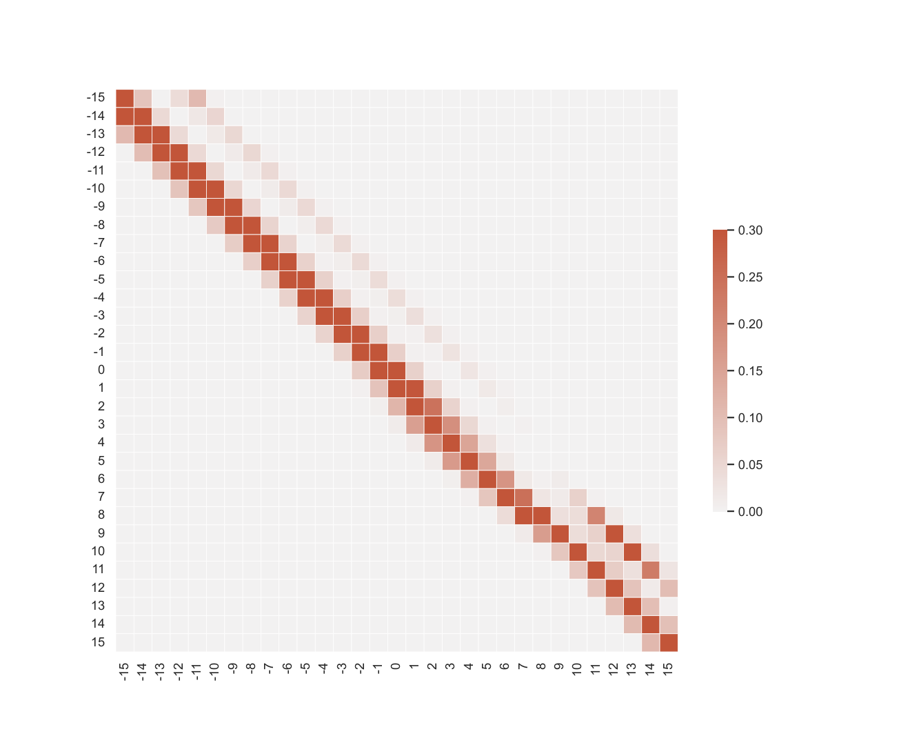
We plot the matrix by diagonal filling approach in Figure 3(a), and the one by uniform filling approach in Figure 3(b). These two approaches do not rely on the available data within the original transition matrix. We can expect their performance to degrade when the training data size becomes smaller.
We plot the matrix by the Gaussian regression recovery approach in Figure 3(c). We find that this approach does not retain the features of the original matrix. Using linear regression to fit the parameters and can result in a large on one side and a small one on the other, as we observe from Figure 3(c). When the current delay is small, the fitted is large. Thus we see that the distribution is more dispersed. When the current delay is large, we even have negative fitted values in the numerical study. For rows with negative fitted values, we let its diagonal be 1. So eventually, this approach leads to a skewed transition matrix, as we see in Figure 3(c).


Table 3 provides the performance comparison for the matrix recovery approaches. Again, we select the median to predict the delay trend, the jump probability to predict the delay jump, and the mean to predict the minutes of delay for these matrix recovery approaches. We find from Table 3 that the Gaussian kernel method achieves the highest score for delay jump prediction, RWMSE, and total score, and a similar score in delay trend prediction as the other filling approaches. This result shows that the Gaussian kernel recovery approach outperforms the other approaches in terms of prediction accuracy. Moreover, this result shows that the good performance of the Gaussian kernel recovery approach is insensitive to the weights given in Equation (12).
| Method | Test Data | RWMSE | Total Score | ||
| Diagonal Filling | Test Set 1 | 0.56947 | 0.48485 | 3.04482 | 4.65101 |
| Test Set 2 | 0.71579 | 0.57143 | 2.86607 | 6.42719 | |
| Uniform Filling | Test Set 1 | 0.57084 | 0.46877 | 3.04449 | 4.49696 |
| Test Set 2 | 0.71665 | 0.48485 | 2.86613 | 5.56580 | |
| Gaussian Regression | Test Set 1 | 0.58557 | 0.47889 | 5.99850 | 1.72371 |
| Test Set 2 | 0.57463 | 0.38724 | 2.65238 | 4.09323 | |
| Gaussian Kernel | Test Set 1 | 0.57231 | 0.56716 | 2.88631 | 5.64684 |
| Test Set 2 | 0.69949 | 0.62500 | 2.58319 | 7.16426 |
5.4 Comparison with Other Time Series Models
We now compare our proposed model with other widely-used time series models.
Naive Prediction Approach
A naive forecasting approach is to assume the delay at station is identical to the current delay, i.e., . This approach does not rely on historical data, and is simple to implement in reality.
Probability Distribution
We can predict the delay at station by simply using its delay distribution. Specifically, we compute for station . We then use the median to predict delay trend, use jump probability to predict delay jump, and delay expectation to predict the minutes of delay.
ARIMA Model
ARIMA model is a linear time series forecasting model that has been used in various forecasting fields, including economics, engineering, and geology (Cryer & Chan 2008). Originated from the autoregressive (AR) model and the moving average (MA) model, the ARIMA model can be used when the time series is stationary and with no missing values (Ediger & Akar 2007). An ARIMA model is usually written as , where is the order of the AR term that refers to the number of lags to be used as predictors. The parameter is the order of the MA term that refers to the number of lagged forecast errors that should go into the ARIMA model. The parameter is the minimum number of differencing needed to make the series stationary.
We implement a nonseasonal ARIMA model with the Python package “pmdarima” (Smith, 2017- 2017-) to predict the delay. We now use Test Set 1 as an example to demonstrate how we develop the ARIMA model. For each train, we use the delays recorded before 8:00 as the training set for the ARIMA model. Then we use the trained model to predict the delay at the predicted station. A detailed description of how to use ARIMA model to predict several time units into the future can be found in Cryer & Chan 2008.
We conduct a stepwise algorithm (Hyndman & Khandakar 2008) to find the optimal model parameters, including the order of AR and the order of MA . We rely on the Akaike’s Information Criterion (AIC) value in selecting the best orders of the ARIMA model. We further obtain the optimal value by conducting differencing tests.
Model Comparison
We compare the prediction scores of the time series model mentioned above in Table 4. Although the naive forecasting approach has the minimum RWMSE, its and scores are the worst since it does not utilize the historical data for training. Using probability distribution to predict delay can be promising when the delay is stable. For instance, its performance for Test Set 2 is close to the performance of our Markov chain model. However, for Test Set 2 whose delays are divergent and unstable, the performance of using probability distribution is much worse than our model. The reason is that the probability distribution is only obtained from historical data. This approach does not utilize the delays at the past stations on the particular predicted date.
The ARIMA model only uses the historical data on the predicted date for training without using the other historical data. When the predicted train’s current station is not far from its starting station 1, the training set could be small so that not much pattern can be learned from history. We can find from Table 4 that the ARIMA model performs worse than the method of using probability distribution due to its training set being small.
The Markov chain model we proposed in this work has a better overall performance than the other models described above. The reason is that the Markov chain model is trained based on historical data and also takes the delay at the current station as the input. Our model has the largest score in . Its score is the best for Test Set 1 where the delays are divergent. Its RWMSE scores are close to the minimal scores given by the naive forecasting approach. We can then conclude that the good performance of our model is not sensitive to the weights assigned in Equation (12).
| Method | Test Data | RWMSE | Total Score | ||
| Naive Forecasting | Test Set 1 | 0.18156 | 0.00476 | 2.86511 | -1.95253 |
| Test Set 2 | 0.24182 | 0.00111 | 2.45632 | -1.23613 | |
| Probability Distribution | Test Set 1 | 0.43879 | 0.53488 | 4.00108 | 3.54168 |
| Test Set 2 | 0.64149 | 0.64849 | 2.58138 | 7.11094 | |
| ARIMA Model | Test Set 1 | 0.39252 | 0.28000 | 3.44114 | 1.32148 |
| Test Set 2 | 0.67438 | 0.42424 | 2.60824 | 5.00610 | |
| Our Model | Test Set 1 | 0.57231 | 0.56716 | 2.88631 | 5.64684 |
| Test Set 2 | 0.69949 | 0.62500 | 2.58319 | 7.16426 |
6 Conclusion and Future Research
This research proposes a novel, accurate, and efficient model to predict railway delays using a Markov-chain-based framework. Theoretical properties of the proposed model are rigorously investigated, and insights are developed. Moreover, we conduct numerical experiments to verify the prediction accuracy and efficiency using the Netherlands Railways data. The major findings of this paper are summarized below:
- •
We propose a non-homogeneous Markov chain to characterize the delay process over stations. To test the order of the Markov chain, we propose and conduct a chi-square Markov property test with the Netherlands Railways data. The results show that the delays over stations of the same train follow a first-order Markov chain.
- •
We develop a Gaussian-kernel-based method to recover the transition matrices for the Markov chain model when the size of training data is small. The Markov chain model equipped with the proposed recovery method achieves a higher prediction accuracy than being with other heuristic matrix recovery methods.
- •
We conduct numerical experiments on the real-world Netherlands Railways data and measure the prediction performance of each implemented model using a certain score calculated with the delay trend, the delay jump, and the root weighted mean square error. The proposed model provides a higher prediction score than other benchmark time series prediction models.
Our investigation of the Markov-chain-based delay prediction model leads to some potential research works. For instance, the strategies for train scheduling and passenger assignment can be improved when considering the potential railway delay (Xu et al. 2019; Li et al. 2020). Incorporating delay prediction into online railway scheduling and dispatching is one of our future research directions. Besides, we can migrate the proposed Markov property test, Markov chain model, and matrix recovery method to other application areas, such as health prognostics (Ghamlouch et al. 2018) and electric load prediction (Khashei & Chahkoutahi 2021).
References
- Aalen & Johansen (1978) Odd. Aalen and Søren Johansen “An empirical transition matrix for non-homogeneous Markov chains based on censored observations” In Scandinavian Journal of Statistics 5.3 JSTOR, 1978, pp. 141–150 URL: http://www.jstor.org/stable/4615704
- Anderson & Goodman (1957) Theodore Anderson and Leo Goodman “Statistical inference about Markov chains” In The Annals of Mathematical Statistics 28.1 JSTOR, 1957, pp. 89–110 URL: https://www.jstor.org/stable/2237025
- Anily & Federgruen (1987) Shoshana Anily and Awi Federgruen “Ergodicity in parametric nonstationary Markov chains: An application to simulated annealing methods” In Operations Research 35.6 INFORMS, 1987, pp. 867–874 URL: https://pubsonline.informs.org/doi/abs/10.1287/opre.35.6.867
- Bickenbach & Bode (2003) Frank Bickenbach and Eckhardt Bode “Evaluating the Markov property in studies of economic convergence” In International Regional Science Review 26.3 Sage Publications, 2003, pp. 363–392 URL: https://doi.org/10.1177/0160017603253789
- Cryer & Chan (2008) Jonathan Cryer and Kung-Sik Chan “Time Series Analysis: With Applications in R” Springer, 2008 URL: https://link.springer.com/book/10.1007/978-0-387-75959-3#bibliographic-information
- Dobrushin (1956) Roland’vovich Dobrushin “Central limit theorem for nonstationary Markov chains. I” In Theory of Probability & Its Applications 1.1 SIAM, 1956, pp. 65–80 URL: http://mi.mathnet.ru/eng/tvp/v1/i1/p72
- Dobrushin (1956a) Roland’vovich Dobrushin “Central limit theorem for nonstationary Markov chains. II” In Theory of Probability & Its Applications 1.4 SIAM, 1956, pp. 329–383 URL: http://mi.mathnet.ru/eng/tvp/v1/i4/p365
- Ediger & Akar (2007) VolkanS Ediger and Sertac Akar “ARIMA forecasting of primary energy demand by fuel in Turkey” In Energy Policy 35.3 Elsevier, 2007, pp. 1701–1708 URL: https://www.sciencedirect.com/science/article/pii/S0301421506002291
- Flier et al. (2009) Holger Flier, Rati Gelashvili, Thomas Graffagnino and Marc Nunkesser “Mining railway delay dependencies in large-scale real-world delay data” In Robust and online large-scale optimization Springer, 2009, pp. 354–368 URL: https://link.springer.com/chapter/10.1007/978-3-642-05465-5_15
- Ge et al. (2021) Meng Ge et al. “ARIMA-FSVR hybrid method for high-speed railway passenger traffic forecasting” In Mathematical Problems in Engineering 2021.9961324 Hindawi, 2021 URL: https://www.hindawi.com/journals/mpe/2021/9961324/
- Ghamlouch et al. (2018) Houda Ghamlouch, Mitra Fouladirad and Antoine Grall “Prognostics for non-monotonous health indicator data with jump diffusion process” In Computers & Industrial Engineering 126 Elsevier, 2018, pp. 1–15 URL: https://www.sciencedirect.com/science/article/pii/S036083521830425X
- Goverde (2005) Rob.P. Goverde “Punctuality of railway operations and timetable stability analysis” In Doctoral thesis, The Netherlands TRAIL Research School, 2005 URL: http://resolver.tudelft.nl/uuid:a40ae4f1-1732-4bf3-bbf5-fdb8dfd635e7
- Harris et al. (2013) Nigel. Harris, Christian. Mjøsund and Hans Haugland “Improving railway performance in Norway” In Journal of Rail Transport Planning & Management 3.4 Elsevier, 2013, pp. 172–180 URL: https://www.sciencedirect.com/science/article/pii/S2210970614000134
- Huang (1977) Cheng-Chi Huang “Non-homogeneous Markov chains and their applications” In Doctoral dissertation, Iowa State University, 1977 URL: https://dr.lib.iastate.edu/handle/20.500.12876/80511
- Huang et al. (2020) Ping Huang et al. “A deep learning approach for multi-attribute data: A study of train delay prediction in railway systems” In Information Sciences 516, 2020, pp. 234–253 URL: https://www.sciencedirect.com/science/article/pii/S0020025519311715
- Hyndman & Khandakar (2008) Rob. Hyndman and Yeasmin Khandakar “Automatic time series forecasting: the forecast package for R” In Journal of Statistical Software 27.3, 2008, pp. 1–22 URL: https://www.jstatsoft.org/index.php/jss/article/view/v027i03
- Khashei & Chahkoutahi (2021) Mehdi Khashei and Fatemeh Chahkoutahi “A comprehensive low-risk and cost parallel hybrid method for electricity load forecasting” In Computers & Industrial Engineering 155 Elsevier, 2021, pp. 107182 URL: https://www.sciencedirect.com/science/article/pii/S0360835221000863
- Koch (1988) Karl-Rudolf Koch “Parameter estimation and hypothesis testing in linear models” Springer, 1988, pp. 306 URL: https://link.springer.com/book/10.1007/978-3-662-03976-2
- Lee et al. (2016) Wei-Hsun Lee, Li-Hsien Yen and Chien-Ming Chou “A delay root cause discovery and timetable adjustment model for enhancing the punctuality of railway services” In Transportation Research Part C: Emerging Technologies 73, 2016, pp. 49–64 URL: https://www.sciencedirect.com/science/article/pii/S0968090X16302005
- Lessan et al. (2019) Javad Lessan, Liping Fu and Chao Wen “A hybrid Bayesian network model for predicting delays in train operations” In Computers & Industrial Engineering 127 Elsevier, 2019, pp. 1214–1222
- Li et al. (2020) Xiaojuan Li et al. “Optimizing train frequencies and train routing with simultaneous passenger assignment in high-speed railway network” In Computers & Industrial Engineering 148 Elsevier, 2020, pp. 106650 URL: https://www.sciencedirect.com/science/article/pii/S0360835220303843
- Li et al. (2021) ZhongCan Li et al. “Near-term train delay prediction in the Dutch railways network” In International Journal of Rail Transportation 9.6 Taylor & Francis, 2021, pp. 520–539 URL: https://doi.org/10.1080/23248378.2020.1843194
- Lippi et al. (2013) Marco Lippi, Matteo Bertini and Paolo Frasconi “Short-term traffic flow forecasting: An experimental comparison of time-series analysis and supervised learning” In IEEE Transactions on Intelligent Transportation Systems 14.2 IEEE, 2013, pp. 871–882 URL: https://ieeexplore.ieee.org/document/6482260
- Ma et al. (2020) Tao Ma, Constantinos Antoniou and Tomer Toledo “Hybrid machine learning algorithm and statistical time series model for network-wide traffic forecast” In Transportation Research Part C: Emerging Technologies 111 Elsevier, 2020, pp. 352–372 URL: https://www.sciencedirect.com/science/article/pii/S0968090X19303821
- Markovi\’c et al. (2015) Nikola Markovi\’c, Sanjin Milinkovi\’c, Konstantin Tikhonov and Paul Schonfeld “Analyzing passenger train arrival delays with support vector regression” In Transportation Research Part C: Emerging Technologies 56 Elsevier, 2015, pp. 251–262 URL: https://www.sciencedirect.com/science/article/pii/S0968090X1500145X
- Nabian et al. (2019) Mohammad Nabian, Negin Alemazkoor and Hadi Meidani “Predicting near-term train schedule performance and delay using bi-level random forests” In Transportation Research Record 2673.5 SAGE Publications Sage CA: Los Angeles, CA, 2019, pp. 564–573 URL: https://journals.sagepub.com/doi/abs/10.1177/0361198119840339
- Olsson & Haugland (2004) Nils.E. Olsson and Hans Haugland “Influencing factors on train punctuality–results from some Norwegian studies” In Transport Policy 11.4 Elsevier, 2004, pp. 387–397 URL: https://www.sciencedirect.com/science/article/pii/S0967070X04000332
- Oneto et al. (2018) Luca Oneto et al. “Train delay prediction systems: a big data analytics perspective” In Big data research 11 Elsevier, 2018, pp. 54–64 URL: https://www.sciencedirect.com/science/article/pii/S2214579617300060
- Pearson (1900) Karl Pearson “X. On the criterion that a given system of deviations from the probable in the case of a correlated system of variables is such that it can be reasonably supposed to have arisen from random sampling” In The London, Edinburgh, and Dublin Philosophical Magazine and Journal of Science 50.302 Taylor & Francis, 1900, pp. 157–175 URL: https://doi.org/10.1080/14786440009463897
- [1] “Railway Statistics 2015 Report”, 2015 International Union of Railways URL: https://uic.org/IMG/pdf/synopsis_2015_print_5_.pdf
- Silverman (2017) Bernard Silverman “Density estimation for statistics and data analysis” Routledge, 2017 URL: https://www.taylorfrancis.com/books/mono/10.1201/9781315140919/density-estimation-statistics-data-analysis-silverman
- Smith, 2017- Taylor. Smith “pmdarima: ARIMA estimators for Python” Online; accessed 2022-05-13, 2017- URL: http://www.alkaline-ml.com/pmdarima
- Suwardo et al. (2010) W Suwardo, Madzlan Napiah and Ibrahim Kamaruddin “ARIMA models for bus travel time prediction” In Journal of the Institute of Engineers Malaysia, 2010, pp. 49–58 URL: https://www.semanticscholar.org/paper/ARIMA-MODELS-FOR-BUS-TRAVEL-TIME-PREDICTION-Suwardo-Madzlan/b2c16e5eb4efbafbd7f8ca3f93eb1a13f31f7677
- Tan & Yilmaz (2002) Baris Tan and Kamil Yilmaz “Markov chain test for time dependence and homogeneity: an analytical and empirical evaluation” In European Journal of Operational Research 137.3 Elsevier, 2002, pp. 524–543 URL: https://ideas.repec.org/a/eee/ejores/v137y2002i3p524-543.html
- Tharwat (2021) Alaa Tharwat “Classification assessment methods” In Applied Computing and Informatics 17.1 Emerald Publishing Limited, 2021, pp. 168–192 URL: https://www.emerald.com/insight/content/doi/10.1016/j.aci.2018.08.003/full/html
- The Institute for Operations Research and the Management Sciences (2018) The Institute for Operations Research and the Management Sciences “2018 RAS Problem Solving Competition: Train Delay Forecasting.”, 2018 URL: https://connect.informs.org/railway-applications/new-item3/problem-solving-competition681
- van der Walt & Bean (2022) Anieke van der Walt and Wilna. Bean “Inventory management for the in-flight catering industry: A case of uncertain demand and product substitutability” In Computers & Industrial Engineering 165, 2022, pp. 107914 URL: https://www.sciencedirect.com/science/article/pii/S0360835221008184
- Xu et al. (2019) Xiaoming Xu, Keping Li and Xiaoshan Lu “Simultaneous locomotive assignment and train scheduling on a single-track railway line: A simulation-based optimization approach” In Computers & Industrial Engineering 127 Elsevier, 2019, pp. 1336–1351 URL: https://www.sciencedirect.com/science/article/pii/S0360835217305223
- Yaghini et al. (2013) Masoud Yaghini, Mohammad Khoshraftar and Masoud Seyedabadi “Railway passenger train delay prediction via neural network model” In Journal of Advanced Transportation 47.3 Wiley Online Library, 2013, pp. 355–368 DOI: 10.1002/atr.193
- Yu et al. (2010) Lei Yu et al. “A nonstationary Markov transition model for computing the relative risk of dementia before death” In Statistics in medicine 29.6 Wiley Online Library, 2010, pp. 639–648 URL: https://www.ncbi.nlm.nih.gov/pmc/articles/PMC2830381/
- Zhang (2003) G.Peter Zhang “Time series forecasting using a hybrid ARIMA and neural network model” In Neurocomputing 50 Elsevier, 2003, pp. 159–175 URL: https://www.sciencedirect.com/science/article/pii/S0925231201007020