Nonparametric Decentralized Detection and Sparse Sensor Selection via Multi-Sensor Online Kernel Scalar QuantizationJ. Guo, D. J. Love, and C. G. Brinton are with the School of Electrical and Computer Engineering, Purdue University, IN 47907 USA. email: richie89311@gmail.com; {djlove, cgb}purdue.eduR. Raj is with the U.S. Naval Research Laboratory, DC 20375 USA. email: raghu.g.raj@gmail.com
Abstract
Signal classification problems arise in a wide variety of applications, and their demand is only expected to grow. In this paper, we focus on the wireless sensor network signal classification setting, where each sensor forwards quantized signals to a fusion center to be classified. Our primary goal is to train a decision function and quantizers across the sensors to maximize the classification performance in an online manner. Moreover, we are interested in sparse sensor selection using a marginalized weighted kernel approach to improve network resource efficiency by disabling less reliable sensors with minimal effect on classification performance. To achieve our goals, we develop a multi-sensor online kernel scalar quantization (MSOKSQ) learning strategy that operates on the sensor outputs at the fusion center. Our theoretical analysis reveals how the proposed algorithm affects the quantizers across the sensors. Additionally, we provide a convergence analysis of our online learning approach by studying its relationship to batch learning. We conduct numerical studies under different classification and sensor network settings which demonstrate the accuracy gains from optimizing different components of MSOKSQ and robustness to reduction in the number of sensors selected.
Index Terms - online learning, wireless sensor network, quantization, joint optimization, kernels, marginalized weighted kernel.
I Introduction
Wireless sensor networks (WSNs), which leverage a set of spatially distributed sensors to sample and process data from an environment, have been extensively studied in the past few decades [1, 2, 3, 4, 5, 6, 7, 8, 9, 10, 11, 12, 13, 14, 15, 16]. A variety of WSN applications in, e.g., wireless communications [1, 2, 3, 4, 5, 6, 7, 8, 9, 10] and radar [11] are increasingly having a significant impact our day-to-day lives. This widespread use of WSNs is driving research in a number of directions. Of particular continuing interest is leveraging WSNs to provide detection/estimation of one or more underlying phenomena, specifically for signal classification tasks [13, 14, 15, 16, 12]. Several works have studied wireless signal classification and related problems in non-WSN settings as well, i.e., where the observations are centralized [17, 18].
In this paper, we focus on decentralized detection [19, 20, 21, 22, 13, 14, 15, 16, 12, 23, 24] exploiting a compress-and-forward sensor network [5, 6, 7, 8, 9, 10, 2, 3, 4, 12]. In this setting, each sensor forwards information resulting from a local decision rule to a fusion center for further processing and decision-making. Decentralized detection problems can be divided into parametric [20, 21, 22] and non-parametric categories [13, 14, 15, 16, 12, 23, 24]. A parametric decentralized detection problem assumes that a fusion center knows or partially knows the joint distribution of (a random vector) and (a random variable), denoted as , where is the observation vector made by the sensors and is the class label of . However, the need to maintain accurate estimates of could lead to performance limitations and an increase in system complexity [13, 14]. Thus, non-parametric decentralized detection is a desirable alternative.
We are interested specifically in non-parametric decentralized detection for signal classification tasks. In the past, authors have approached this topic by leveraging kernel-based learning techniques, e.g., [13, 14, 12, 15, 16]. Kernel methods are commonly employed to reduce computational complexity in problems that require mapping non-linearly separable datasets to higher dimensional spaces for decision learning [13, 14, 12, 15, 16]. The scenarios studied in [13, 14, 12] most closely align with our focus in this paper. In these works, each sensor forwards a quantized observation based on a quantization rule (corresponding to a local decision) to a fusion center. Then, the fusion center employs a decision function that maps from the space of quantized observations to the set of real numbers via the kernel being employed. The output of the decision function is used to infer the corresponding signal classification class label. To maximize classification performance, a joint optimization problem with respect to the quantizers (i.e., quantization rules) and the decision function is considered.
The methods in [13, 14] are based on batch learning (BL), where model training is conducted after full batches of data have been collected. For contemporary WSN applications which generate large volumes of observations in short time intervals, BL approaches potentially incur significant computation overhead. Additionally, the detector/estimator learnt by the BL approach is highly dependent on the unknown input training sample distribution, i.e., . If the dataset distribution used for training is mismatched to the current WSN inputs (i.e., the testing dataset), which will happen when the environment evolves over time, the learning performance (e.g., classification accuracy) can be degraded significantly.
In settings where information on the underlying environment exists, e.g., in terms of a finite state space, contemporary methods for modeling system evolution between states over time (e.g., Markov jump processes [25, 26]) could potentially be employed to capture these dynamics and enable the application of BL approaches within particular WSN states. As mentioned previously, we are interested in non-parametric approaches that do not require such assumptions. To address these challenges, one possibility is to consider an online learning (OL) approach to signal classification, where the fusion center adapts the classifier structure dynamically, i.e., each time a new data sample is observed by the sensors.
In this paper, our primary goal is to develop an OL methodology for WSNs that jointly optimizes the quantizers and the decision function dynamically. Our theoretical analysis will also establish relationships between our OL approach and the BL method studied in [13]. In doing so, we will see how the proposed algorithm affects the quantization rules based on some computationally friendly marginalized kernels.
Our prior work [12] developed an OL methodology for signal classification based on measurements from a single sensor. One of the key differences here is the need to coordinate multiple sensors in a WSN. Specifically, it can be expected that quantization outputs will have varying contributions to the signal classifier at the fusion center, e.g., some sensors are naturally less reliable when they are deployed over a large area. To promote higher network operating efficiency, we are thus also interested in sensor selection [14, 27, 28], where a certain number of lowest contributing sensors are disabled. We accomplish this within our OL framework by introducing a marginalized weighted kernel [14] that allows us to assess sensor quality. Compared to more general kernel-based OL methodologies, e.g., [29, 15, 16, 30, 31, 32, 33], we consider the joint optimization of quantization, classification and sensor selection strategies.
Summary of contributions. The main contributions of this paper are summarized as follows:
- •
We introduce a WSN system model for signal classification with sparse sensor selection in the OL setting. We formalize the instantaneous regularized risk for the OL setting in terms of the relevant WSN system parameters: decision function weights, quantization rules, and weighted parameter vectors for sensor selection.
- •
We develop the multi-sensor online kernel scalar quantization (MSOKSQ) algorithm to update our WSN parameters as new measurements are collected over time. Our generalized algorithm is based on alternating (sub-)-gradient methods that leverage the convexity of our risk function with respect to each of the three groups of WSN parameters. We present a specific implementation of our methodology based on a computationally friendly kernel.
- •
We theoretically analyze the convergence behavior of our MSOKSQ algorithm, comparing the risk function to prior BL approaches [13, 14]. We analyze the quantization rule updates across the sensors and obtain conditions on our system parameters under which the quantizers become (approximately) deterministic.
Through numerical evaluation on synthetic and real-world datasets, we demonstrate the impact of different WSN system components on MSOKSQ learning performance. We find that these numerical results validate our theoretical results.
The rest of the paper is organized as follows. Section II introduces the system model and basic background on kernels and decision functions. In Section III, we introduce the risk functions for the BL and OL approaches. The MSOKSQ algorithm is developed based on the marginalized weighted kernel in Section IV. In Section V, we theoretically analyze the quantization rule updates and characterize the convergence behavior of our methodology. Numerical evaluation (including a randomly generated dataset and the multi-class UCI Iris dataset [34]) follows in Section VI. Finally, we conclude the paper and discuss future work.
II System Model and Preliminaries
In this section, we first describe the WSN system model (Section II-A). Then, we provide basic background on kernels and decision functions for our estimation model (Section II-B).
II-A Wireless Sensor Network System Model
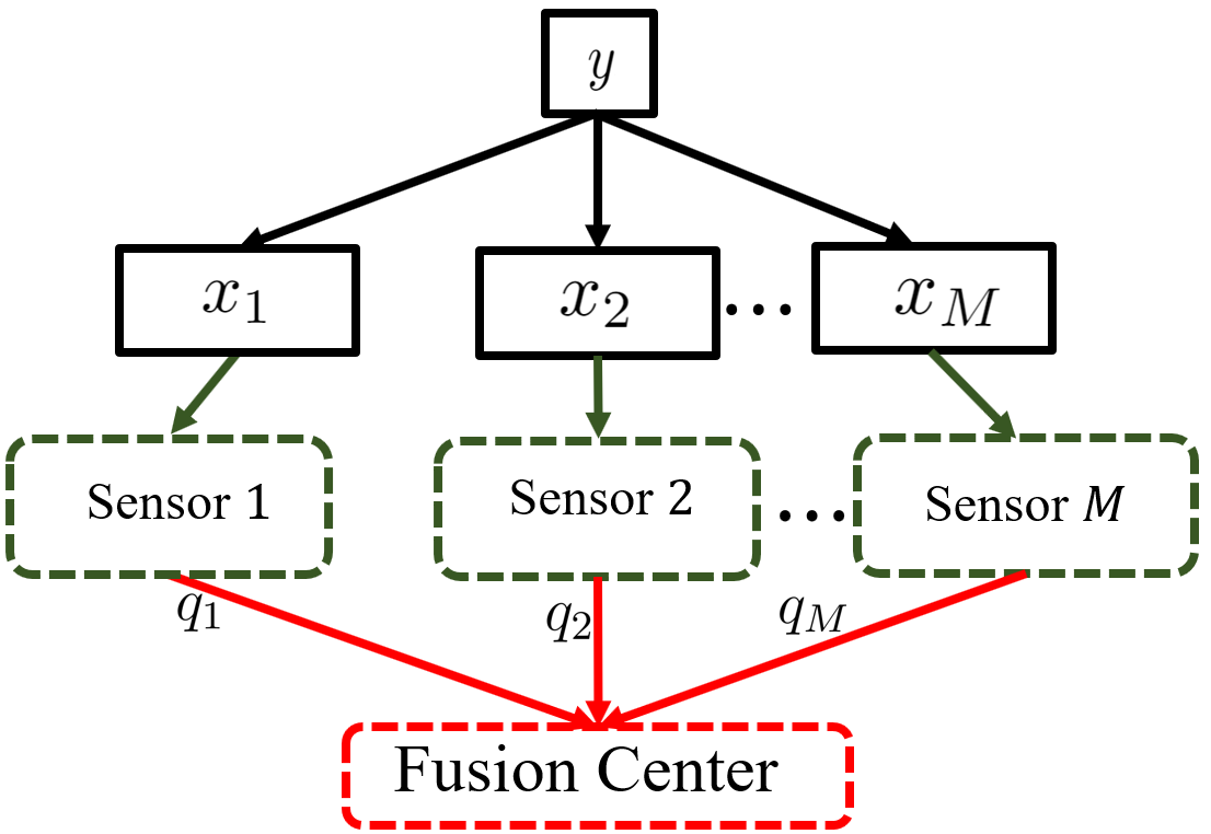
We consider sensors connected to a common fusion center as shown in Fig. 1. Sensor is capable of measuring an observation of the environment, where is finite collection of potential observations by sensor . The fusion center must utilize the sensors to train a decision function to determine the class of a signal being observed by the sensors. We denote this class by representing a model for the target (dependent) variable of interest. Given our focus on signal classification, is considered as a finite discrete set. Although our proposed system model and methods are applicable to any multi-class problem, our presentation will often focus on the the binary classification case for simplicity, i.e., .
We assume perfect synchronization among sensors. The primary functions of the fusion center are: i) training a decision function chosen from a function space to determine the signal class and ii) determining a quantization rule to be employed by each sensor’s quantizer in order to maximize classification performance. To accommodate sensor selection, we consider a third function: iii) utilizing of quantized observations, where , which can promote network resource efficiency through disabling lower quality sensors.
Ideally, the fusion center and quantizers would have access to of the sensor observations and the signal class. Here, is a random variable for the signal class and is the random vector for observations across the sensors . However, as discussed in Section I, this distribution is often unknown and difficult to estimate. To overcome this lack of knowledge, we consider non-parametric decentralized detection based on a sequence of training samples such that is the vector of observations over sensors at time , , and . In the OL setting, this positive integer denotes the number of time instances under consideration, where one sample arrives at each time instance. Note that it is usually treated as the total number of samples in the BL setting, e.g., [13, 14].
We let denote sensor ’s quantized version of at time . Across the sensors, we consider the vector , where . We assume and are finite sets such that , , and , for all . Note that denotes the cardinality of the set . is produced based on the quantization rule of sensor at time . We expect in practice that for a particular value of will be unimodal: Given , there would be one value of where the density is the highest, and it would taper off from there as is varied, e.g., as a Gaussian distribution. According to the axioms of probability [35], these rules must follow and , for all and . We posit conditional independence of the quantization rules at time (which confers computational efficiency to our algorithms) [13, 14]:
| (1) |
for all possible and . As a result, we can form a set of the feasible quantization rules across the sensors as
| (2) |
where is a random vector.
After quantization, the WSN forwards to the fusion center. Similar to [13, 14, 12], we assume that the fusion center perfectly observes , i.e., the channel does not introduce significant noise to the quantized measurements. The fusion center aims to jointly optimize the decision function, quantization rules, and sensor selection, thereby controlling the behavior of the quantizers (i.e., ) at each time .
II-B Kernel and Decision Function
II-B1 Kernel
We are interested in developing an OL algorithm that can work with both linearly and non-linearly separable models of the quantized data. One common approach to dealing with non-linearly separable models is to map the dataset to a high-dimensional space using a mapping function [14, 13, 12, 29, 15, 16, 36]. Generally, this mapping function is not unique. An algorithm can then be developed based on the inner product between points, i.e., for all possible quantization points , for , so that the problem is solved using one or more (approximately) linear decision boundaries [14, 13, 12, 29, 15, 16, 36]. Although it can be computationally challenging to construct , with kernel methods, we work with instead, which is much easier to construct [36].
Definition 1
A real-valued symmetric function is a kernel if the matrix for is positive semidefinite, i.e., a Gram matrix.
We can define the mapping function based on a kernel according to so that To facilitate sensor selection, we focus on weighted kernels in this paper [14]. Specifically, a weighted kernel is used to associate each sensor with a level of reliability using a weight parameter vector that satisfies
| (3) |
where indicates for all . A larger weight indicates that the corresponding sensor is more reliable [14]. Furthermore, we consider sensor to be disabled when . For this reason, the weighted kernel will be critical to our algorithm development. Note that the construction of the weighted kernel is not unique. An example weighted kernel is the weighted count kernel described by [13, 14] 11 1 Another example inspired by [13] is the weighed linear kernel, e.g., .
| (4) |
where denotes the indicator function. and are the th element of and , respectively.
II-B2 Decision function
The purpose of the decision function is to estimate/predict the class of the input samples from the quantized sensor measurements. Formally, the decision function is defined as
| (5) |
where for each quantization point . We assume that is a reproducing kernel Hilbert space (RKHS). A RKHS is one for which there is a kernel such that the following two properties hold:
- •
has the reproducing property
(6) - •
is the closure of the space of all , for all .
We refer to as the weight of . This means that (6) is the decision function induced by the mapping space . In addition, based on (5) and (6).
III Estimation Model
In this section, we formalize the signal classification problem for the BL (Section III-A) and OL (Section III-B) settings.
III-A Prior Work: Batch Learning Problem Formulation
BL has been employed for WSN signal classification in prior works [13, 14, 36]. In BL, training and estimation are conducted after the sample sequence has been collected. This formulation will be useful to us in our subsequent development of the OL case. A solution set for the BL approach can be denoted . The weight of the decision function , the quantization rules across the sensors , and the weight parameter vector are determined offline based on , and thus they will not change over time as compared to the OL case. We use the subscript in the BL setting to denote the sample index.
An empirical risk function was introduced by [13, 14] to obtain the optimal , which is given by
| (7) |
where is a loss function, which can either be a differentiable or non-differentiable convex function. For example, the logistic loss is a differentiable function, which is
| (8) |
On the other hand, the soft margin loss function takes the following non-differentiable form [29]:
| (9) |
where is the margin parameter, , and . (9) becomes the hinge loss function when , which is most notably used for the binary classification problem, e.g., [13, 14, 12, 36].
To prevent model overfitting and perform sensor selection, a regularized form of the empirical risk function was introduced in [14], which is given by
| (10) |
where and denote the and norms, respectively. This same choice of norms will also be used for the OL setting in Section III-B. The regularization parameters are treated as fixed [14]. controls how many reliable sensors are selected for the classification [14], with the norm helping to enforce a sparse solution while retaining convexity.
It is difficult to learn the desired parameters in (10) based on an expectation of the loss function over for all [13, 14]. Traditional upper-bounding techniques impose high computational complexity. To resolve this, [13] and [14] apply Jensen’s inequality to work with the following lower bound of (10):
| (11) |
where is a marginalized mapping function based on [13, 14] for jointly solving and :
| (12) |
Note that (10) and (11) are equal when the quantizers are deterministic [13, 14], i.e.,
| (13) |
for all and sample . The optimal for this deterministic case described in (13) can be derived for both (10) and (11), which has been studied in [13, 14]. Additionally, these works have shown that the lower bound risk (11) converges to (10) for a large training dataset. With this in hand, we move on formulating a risk function for the OL setting, which will build upon (11) for the BL case.
III-B Online Learning Problem Formulation
One of the main contributions of this paper is to solve the decentralized signal classification problem in the online setting. Specifically, we need to update the weight of the decision function , the quantization rules across the sensors , and the weighted parameter vector satisfying (3) at each time , i.e., whenever a new sample is observed. We will use as a solution set sequence across the sensors over time .
For the OL setting, we formulate the following instantaneous regularized risk function, inspired by [14, 29]:
| (14) |
which is an approximation of in (11) based on the sample at time . As before, and are regularization terms. Note that controls how many sensors are disabled which may evolve over time. The modified decision function at time is , inspired by (11). The marginalized mapping function at time is
| (15) |
Compared to (12), can be considered as the mapping function associated with at time . is the weighted kernel with respect to time and . We define as the marginalized kernel with time and for developing an algorithm to solve (14):
| (16) |
The kernel calculation will be the most computationally intensive component of our methodology in Section IV. In general, (16) has a complexity of , which becomes prohibitive for a large number of training samples . To address this, inspired by [13, 12, 14], we will consider a computationally friendly weighted marginalized kernel, namely, the weighted count marginalized kernel [37]:22 2 Another example is the marginalized weighed linear kernel with time and , i.e., , where is th element of the random vector .
| (17) |
This reduces the kernel calculation complexity to , where , and is the number of time instances for which and . More generally, there are several ways to construct , as long as the construction of in (16) follows Definition 1.
Compared to [14], an additional constraint has been added in the indicator , for all because of the OL setting. This change ensures the each sensor quantizer becomes a(n) (approximate) deterministic quantizer in the limit. This is important because, similar to (11) for the BL case, (14) is a lower bound on the risk function for the OL setting. Our theoretical analysis in Section V (Lemma 1, Theorem 2) will establish a relationship between the performance of these two lower bounds, and we will see that they converge once a large number of samples have been observed.
IV Online Learning Methodology
We will now develop our MSOKSQ methodology for the formulation in Section III-B. To do so, we note that while (14) is non-convex with respect to , it is convex with respect to each of the variable sets , , and individually while the other two are assumed to be fixed. Thus, we are motivated to develop a (sub-)gradient descent-based method that minimizes (14) by iteratively updating each element in .
In this paper, we focus on the most general case of non-differential loss functions used in (14), where the sub-gradients of elements in prior to each update need to be derived. We can extend the results of the algorithm to any differentiable loss function since the sub-gradient of a differentiable loss function is its gradient [36].
Procedurally, after we initialize , , and for all possible and , we first must derive three updates. First is to derive given and at time (Section IV-A), where is the updated version of . Second is to derive given and at time (Section IV-B). Finally, we must obtain given and at time (Section IV-C). The resulting procedure is summarized in Algorithm 1.
IV-A Obtaining weight of decision function
Given and , we update based on (14) using
| (18) |
where is the learning rate. is the sub-gradient of with respect to , given by
| (19) |
using the chain rule, where is the updated marginalized mapping function at time
| (20) |
Initializing , we update as
| (21) |
where is the coefficient at time of , which is given by
| (22) |
To form , the new coefficient is generated with based on the sub-gradient of , and the on the previous are multiplied by for as in [29]. Followed by this, we can write the modified decision function, which is given by
| (23) |
We can see from (22) that we need for the updates to converge [29]. Our theoretical analysis in Section V will not make additional assumptions on the value of , which can in general be chosen through cross-validation on a particular dataset.
IV-B Obtaining for all possible and
We derive given and for all possible and some . This is done by first deriving using a conditional (coordinate) sub-gradient method described by [12, 13, 14] for all , some , and . Then, we use the relationship described in (1) to obtain the resulting . Note that is the updated .
The following theorem gives the sub-gradient of with respect to for any weighted marginalized kernel at time , for all .
Theorem 1
Given , , and an i.i.d. sequence for any marginalized weighted kernel defined in (16),
| (24) |
where and are possible quantization outputs across the sensors at time and , respectively, and
| (25) |
Proof:
Using the chain rule, we can write
| (26) |
The first term on the right hand side (RHS) of (26) is defined as shown in (25). The second term on the RHS of (26) is
| (27) |
where (27a) holds based on (16) and (23).
Thus, (24) is obtained by applying (1) and (27a), where
∂_P_m,n(q_m,n—x_m,n)P_n(q_n— x_n) =
P
n
(q
n
—x
n
)
P
m,n
(q
m,n
—x
m,n
)
.
∎
In Theorem 1, we see that the size of the summation for computing the sub-gradient increases exponentially with . To resolve this, the following proposition provides a special form of for the weighted count marginalized kernel in (17).
Proposition 1
Proof:
Since must satisfy the summation constraint described in (2) for all and , we can update to through the conditional sub-gradient method with a simplex constraint [38, 14, 13] from the summation in (2). We focus on (16) for updating because it will enforce quantizers across the sensors to be deterministic after some time instance, which we will provide detailed proof of in Section V-C.
The OL setting considered in this paper has the added complexity of dealing with data over time. Specifically, we update at time based on the input that is observed, as opposed to updating across all possible inputs simultaneously as is the case in the BL setting [13, 14]. Hence, does not necessarily equal the updated version of , i.e., , because may not equal . The goal is to update the quantization rule only when the same input has been observed again.
For this reason, we let denote an index for the number of times has been observed at sensor through the present time . Furthermore, is used to denote the time index of the most recent observation of input at sensor . For example, if , then sensor has observed three times up through time . Though depends on , we omit this in the writing of for notational convenience.
Thus, we must update from time based on (2). Given , we calculate from
| (29) |
Then if the sub-gradient is negative, we have the following update rule inspired by [38, Chapter 2]:
| (30) |
where denotes the signum function. Otherwise, we have
| (31) |
for all in order to strictly satisfy the summation constraint proposed in (2) for all . is the learning rate of the quantization rule at time , which we sometimes write as to emphasize that it would only vary based on the number of times has been observed at sensor . We will see in Section V-C that impacts the rate of convergence to a deterministic quantizer.
Followed by this, the quantization rule when sensor observes for the th time at time is
because . Then, the expression of follows from (1) and the fact that
| (32) |
IV-C Obtaining weighted parameter vector
Finally, we consider obtaining the updated weight parameter vector given and . Recall that the purpose of introducing is for sensor selection, i.e., to properly select the most reliable sensors among all sensors in the classification model. Thus, the OL update considers the design of and the regularization parameter in (11) jointly. The update will be terminated when at most elements of are not .
To make a fair reliability comparison, we initialize and . We update using a conditional sub-gradient method to enforce a sparse solution, e.g., the projection sub-gradient method [38]. For a given weighted marginalized kernel, the sub-gradient of with respect to can be expressed using the chain rule as
| (33) |
where defined by (20) is the updated marginalized mapping function at time and is given by
| (34) |
Using (23), the gradient of the decision function is obtained as
| (35) |
As in Section IV-B, the computational requirement for solving (35) increases with . The following proposition gives an efficient expression for based on the kernel in (17).
Proposition 2
Given , , and an i.i.d. sequence , for the kernel in (17) is
| (36) |
Proof:
We start by writing (33) in terms of (34) and (35). Using (17), we obtain the following expression for (35):
| (37) |
With this in hand, we can employ a projected sub-gradient method to update while satisfying the constraint in (3). Given the objective of selecting sensors to be kept on, the update is terminated once we reach a time instance such that elements of are zero. Specifically, at time , to get a sparse solution, we update
| (38) |
to maintain constraint (3), where is the count of the number of non-zero elements, and the th element of is
| (39) |
where is learning rate with respect to . controls the training time prior to disabling sensors. As the value of is increased, this time will be shortened. To ensure that exactly sensors are enabled, we can design the regularization constant such that at most one sensor is set to zero in (38) at each time :
| (40) |
There are also other potential settings for which will result in while yielding possibly different values of . Other conditional sub-gradient methods can be used as long as the sparse solution is enforced.
Algorithm 1 summarizes the entire MSOKSQ procedure developed throughout this section. In practice, this algorithm will continue running indefinitely, with the value of incrementing each time a new collection of measurements is generated across the sensors. For the weighted count marginalized kernel (17), Propositions 1 and 2 indicate that the quantization rule and weight parameter updates can be done independently at time across each sensor .
V Theoretical Analysis
In this section, we theoretically analyze our MSOKSQ algorithm. We first provide assumptions for the OL and BL approaches similar to [29, 13, 14] (Section V-A). Then, we study the relationship between the OL and BL approaches (Section V-B). Followed by this, we will characterize the update behavior of the quantization rules and sensor weights from MSOKSQ in the OL setting (Section V-C). Finally, we conduct a convergence analysis that compares the OL and BL approaches (Section V-D).
V-A Definitions and Assumptions
Consider a fixed i.i.d. sequence of measurements . We assume there is a such that the marginalized mapping functions of the BL and OL settings in (12) and (15) satisfy , for all and . Additionally, we assume that derived by the BL approach is bounded such that for any , where
| (42) |
The value of is derived based on the loss function which we assume satisfies the Lipschitz condition [29]:
| (43) |
where and . Hence, for the OL approach, given , we bound for , which follows from based on (18) and (19) for all possible and . As we set and , we obtain from (18).
The learning rate for can be chosen to be where , which is a standard setting found in OL problems, e.g., [12, 15, 16, 29] due to its theoretical guarantees. This setting is desirable in our problem given the convergence bound relationships it will produce with prior batch learning training approaches, as we will see in Section V-D.
Finally, we define a set that contains (i) all possible solutions for the OL setting, as well as (ii) all possible solutions for the BL setting. Moreover, we consider a set for the deterministic quantizer such that the weights of the decision function and the weighted parameter vector are jointly derived based on the rules defined in (13), for both the OL and the BL setting.
V-B Connecting OL and BL Approaches
We quantitatively compare the behavior of our OL methodology to previously studied BL approaches [13, 14]. Following prior work on OL [29, 15, 16, 36], we will compare the average instantaneous regularized risk function for the OL setting, i.e.,
| (44) |
with for the BL setting defined in (11).
Before we make the connection, we first define
| (45) |
to be the OL risk function defined in (14) for a constant weight on decision function [29], i.e., the BL case. Due to the convexity of , we know that . Thus, the inequality
| (46) |
from [29] holds for our setting. With this inequality, we obtain the following lemma:
Lemma 1
Given an i.i.d. sequence of time samples, suppose Algorithm 1 is executed with and . For any solution set sequence , we have
| (47) |
where is Big notation, for some .
Proof:
We first show the sequence of inequalities in (48).
| (48) |
Inspired by [29], we obtain (48a) by adding The first three terms on the RHS of (48b) are derived using as shown in [29] and (46). The fourth term holds because from the triangle inequality, and . Given this, we derive (48c) using
| (49) |
where (49a) follows from Jensen’s inequality and the fact that the weights of and are the same, and (49b) follows from (43) and the Cauchy Schwartz inequality. Finally, note that
| (50) |
based on the facts and . Then, (47) is justified considering (48) and (50). ∎
Lemma 1 establishes a relationship between the risk function of the OL and BL approaches: there is a gap between and when there is a larger variance in the marginalized mapping function and sensor selection weights over time. We next explore how our update rules in Algorithm 1 can further refine the bound in (47).
V-C Quantization Rules and Weight Parameter Vector Analysis
In (47), the first term is dependent on the quantization rules and the weighed parameter vector while the second term relates to the weight parameter vector. We are thus interested to study how Algorithm 1 affects the updates of the quantization rules and the weighted parameter vector over time. In our analysis, we will assume the soft margin loss function (9) for the binary classification problem.
The quantization rules across the sensors have significant impacts on the classification performance, as we will show numerically in Section VI. Prior works in decentralized signal detection [13, 12, 14] have not considered the effect of quantization rules. Thus, we are interested in studying the update behaviors of the quantization rules based on the weighted count marginalized kernel in (17). Before we provide our Proposition 3, some facts need to be addressed.
Recall is the time index at which sensor observes the -th instance of . The values of and in (22) and (25) are affected by defined in (9). For any , considering (22), (25), (28), and (41), we have that
| (51) |
This indicates from (28) that
| (52) |
Hence, the update of occurs when , for some . Specifically, is increased by while , i.e., for all other is reduced by based on (30). is defined in (29).
As we expect for a particular value of to be unimodal in practice, we initialize
| (53) |
for , , and for all .
Proposition 3
Proof:
This proof starts with generalizing the expression of , which is given by
| (56) |
using (30), (29), (51)-(53), and (55). Followed by this, we use (2) to obtain ∎Based on Proposition 3, if we set the learning rate for all , the quantizer of sensor will become a deterministic quantizer with respect to observation once . In this case, the quantization rules of the sensors become the same, and the sensor selection strategy is effectively disabled, since it relies on quantizer diversity. More generally, if for all and , the quantizer approaches deterministic behavior asymptotically as the number of observations increases, with larger producing a faster rate of convergence. Our numerical experiments in Section VI will confirm that convergence is reached even for small values of .
Since our primary goal is to train the decision function and the quantization rules across the sensors, we are also interested in the case when the sensor selection strategy is not used (i.e., ). Additionally, the algorithms proposed by [13] and [14] are the same when and is fixed. Hence, we can compare from our OL setting with defined in [13] when and , which indicates that
| (57) |
where and correspond to the OL and BL settings, respectively. Based on this, we next aim to analyze the performance of our OL methodology against that of the BL setting assuming the BL optimal solution drawn from .
V-D Convergence Analysis
We will now leverage Proposition 3 to tighten our result in Lemma 1. In doing so, we will assume the sensor selection strategy is not employed, which makes our OL setting directly comparable to prior work [13] for the BL approach as discussed above. In these works, the relationship between the true risk function and the empirical risk function of the BL approach (i.e., the first term on the RHS of (11)) have been shown to follow
| (58) |
where is the optimal solution of the true risk function assuming the fusion center and all sensors know . indicates that
| (59) |
The following theorem shows that a similar relationship exists between from the OL approach and from the BL approach.
Theorem 2
Consider the soft margin loss in (9) with a properly selected as in Proposition 3, , and an i.i.d. sequence such that all sensors have observed all possible at least times at time . Furthermore, suppose , and , for all . If the quantization rules of the OL approach are initialized as in (53), and the deterministic quantization rules of the BL approach described in (13) follow (53), then, for large ,
| (60) |
where
| (61) |
and is defined by Proposition 3.
Proof:
Given the fact that and for all , (47) can be re-written based on Lemma 1 as
| (62) |
The norm in (62) can be written as
| (63) |
where (63) follows (57). Note that and are quantization rules across the sensors with respect to the OL and BL approaches, respectively.
At time , each sensor has observed all possible at least times. Thus, once , we can approximate the quantization rules across the sensors based on Proposition 3 and (2) as
| (64) |
for a fixed . Now, writing
| (65) |
we can approximate
| (66) |
by the triangle inequality and for large , and
| (67) |
using (63) and the fact that the initialized quantization rules of the OL and the deterministic quantization rules of the BL follow (53). (60) then follows from (66) and (67). ∎
Note that in the case when , (60) can be written based on Proposition 2 as
| (68) |
Comparing Theorem 2 and Lemma 1, the performance of our OL methodology converges to that of BL setting [29] assuming the BL optimal solution belonging to is considered.
Remark 1
Placing a deterministic quantizer at each sensor indicates that the size of would be reduced to . In this case, for any , the class label of would always the same as that of , where is the corresponding quantization output of . Thus, we are also interested in analyzing the classification performance between a bit deterministic quantizer and an infinite-resolution deterministic quantizer. In this paper, each sensor using an infinite-resolution deterministic quantizer would imply that the quantization operation can be neglected, i.e., and that the sensors are equally reliable. In this particular setting, Algorithm 1 can be seen as the native online regularized-risk minimization algorithm (NORMA) [29]. NORMA described by [29] trains the weights of the decision function that can be implemented in the proposed multi-sensor model. Given the fact that the classification performance of NORMA [29, Theorem 4] is approximately equal to the BL setting when infinite-resolution deterministic quantizers are considered, we use NORMA as the an upper bound on achievable performance of MSOKSQ in Section VI.
VI Numerical Performance Analysis
We will now conduct a numerical evaluation of our MSOKSQ methodology. We will consider two datasets for classification tasks distributed across sensors: a 2-class randomly generated dataset (Section VI-B), and the 3-class Iris dataset from the University of California, Irvine (UCI) open source repository [34] (Section VI-C). Before presenting these results, we will discuss our evaluation setup (Section VI-A).
VI-A Simulation Setup
In each experiment, we set the learning rates for to (satisfying the conditions in Lemma 1 and Theorem 2), to , and to . For regularization parameters, we set (which satisfies the constraint from (22) for each ), and according to (40). We find that these settings lead to stable training performance. Additionally, we use a margin parameter (hinge loss). We initialize , , and based on (53). The simulations are done using the weighted count marginalized kernel in (17).
Inspired by [39], we define the quantization points as uniform partitions over the range , i.e.,
| (69) |
To evaluate the performance of MSOKSQ, we consider several baselines/variants of Algorithm 1:
- •
- •
MSOKSQ without updating and : This can be considered as NORMA because and are not being updated by Algorithm 1 for all .
- •
- •
MSOKSQ with -bit deterministic quantizer: In this case, Algorithm 1 is executed assuming for all .
- •
MSOKSQ optimally selects : Here, Algorithm 1 is performed given sensors need to be enabled.
- •
MSOKSQ randomly selects : Here, sensors are randomly enabled, which can be done by reassigning the value of produced by Algorithm 1 randomly.


VI-B Binary Classification Problem from Synthetic Data
We first consider a binary classification task, i.e., . In our evaluation, we aim to emulate different degrees of (i) measurement variation across sensors and (ii) separability of the dataset between classes. To do so, we generate elements of for sensor according to
| (70) |
where is a constant and is sampled from a uniform distribution over for each measurement. In this way, each , and the observation sets are each unique. At time , observation is assumed to be randomly selected from .
Note that we can vary the degree to which the classes are separated through proper selection of . For example, at a single sensor , Fig. 2 shows the construction of with 100 data points, where 50 points are generated for each class, for and . Fig. 3 shows samples generated over time for each of the in Fig. 2. We see that with is a linearly separable dataset while with is non-separable.
In the following simulations, we consider time instances. We assume that is initialized based on (2) for all possible and . By default, each sensor is equipped with a -bit uniform quantizer, where is defined in (69). The observation set for sensor is generated according to (70) with and data points/class. The fusion center first classifies the quantization outputs forwarded by the sensors using
| (71) |
where follows the weighted count kernel in (4). Then, the fusion center updates the solution based on Section IV. The accuracy classification rate (ACR) is used as our classification performance metric, which is
| (72) |
for . This metric quantifies the signal classification accuracy of the WSN over time, which allows us to assess the performance of our online learning methodology and compare the impact of different components of our algorithm (i.e., the quantization, sensor selection, and decision function updates). Similar metrics (e.g., error rate, total loss) have been employed in prior works for decentralized OL [29, 16].
In Fig. 4, we study how the number of sensors and optimization of the quantization rules affect the ACR performance. We consider the number of sensor and . We assume that in (70), i.e., the dataset is non-separable. We see that ACR for both MSOKSQ without updating and MSOKSQ without updating and increase with the number of sensors. As the time instance increases, MSOKSQ without updating begins to offer substantial improvements in ACR performance over MSOKSQ without updating and (up to 20% by ), which demonstrates the importance of optimizing the quantization rules. Moreover, the ACR performance of MSOKSQ without updating approaches the ACR performance of NORMA in the limit because the randomized quantizers become deterministic quantizers (Proposition 3). Further, when each sensor uses a 1-bit deterministic quantizer, the ACR performance of MSOKSQ overlaps that of NORMA, as we discuss in Remark 2 below.
Remark 2
Sensors are equally reliable when deterministic quantizers are considered. As Fig. 4, Fig. 5, and Fig. 7 Fig. 9 show, if we properly select the precision of the deterministic quantizers, i.e., , for all , the ACR performance of the -bit deterministic quantizer achieves the same performance as NORMA.
Fig. 5 analyzes the ACR performance for both optimal and random sensors selections when the total number of sensor is . We include three different cases of and sensors enabled, given sensors equip -bit quantizers. We see that the ACR performance of MSOKSQ increases over time for both optimal and random sensor selection strategies, with optimal sensor selection outperforming random sensor selection for all choices of . Also, while the performance decreases when decreases, we see that our optimization strategy provides ACR robustness as the available sensor selection budget changes from to . Additionally, we see that the ACR performance of MSOKSQ optimal/random sensor selections approach NORMA as the time instance increases for all . As in Fig. 4, this is due to the fact that the randomized quantizers become deterministic in the limit. Finally, when each sensor uses a 2-bit deterministic quantizer, we see that the ACR performance of MSOKSQ overlaps NORMA, consistent with Remark 2.
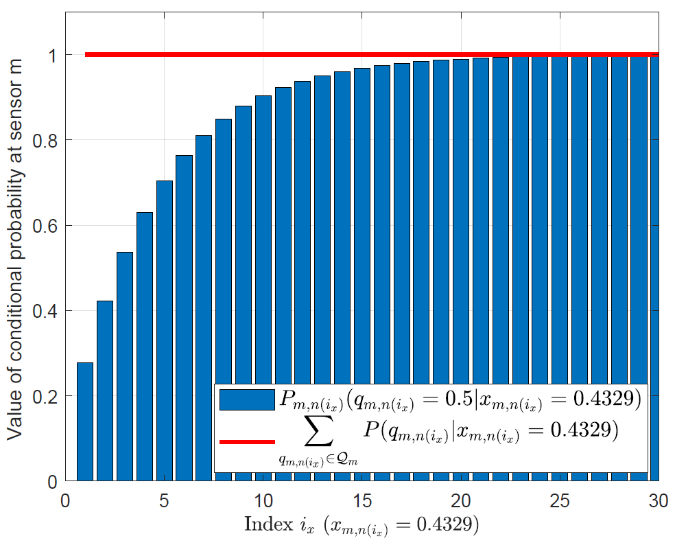
Fig. 6 demonstrates the quantization rule behavior of MSOKSQ at a particular value of (). The settings in of Fig. 6 are the same as Fig. 5. Given defined in (69), the quantization rule of sensor is initialized such that
| (73) |
Fig. 6 indicates that approaches 1 with (the number of times has been observed). Thus, Fig. 6 is consistent with Proposition 3.



VI-C Multi-Class Classification Problem on Iris Dataset
Although our presentation throughout the paper has focused binary classification, Algorithm 1 can handle multi-class classification as well. In the 3-class Iris dataset [34], each Iris plant belongs to one of three classes , and thus for each sample in our setting. We assume that the observation set for each sensor is the petal width of the Iris plants such that . If we assume each sensor equips a 2-bit quantizer, then the quantization points are [39]. Over time instances, each sensor makes its observations that are assumed to be drawn from randomly per time instance, for all .
To address multi-class within our methodology, we will employ the standard One Versus All (OVA) technique, where a decision function is trained for each label dimension separately [36, 40, 41]. At each time instance , then, the update in Algorithm 1 is run once for each decision function independently. In the Iris setting, we need two decision functions, where the first and the second decision functions classify the first label, , and the second label, , respectively. The ACR for the multi-class problem is defined in (74), where and are the weights of the decision functions that will be use to determine , for .
| (74) |
Fig. 7 demonstrates how the number of quantization bits affects the ACR for the multi-class problem. We assume the total number of sensor is . We compare the cases when each sensor produces 1-bit and 2-bit outputs assuming and sensors are enabled. Initially, the ACR performance of the 1-bit quantizer exceeds that of the 2-bit quantizer because the quantization rules of the 1-bit quantizer become deterministic faster than the 2-bit quantizer. However, a -bit quantizer maps onto one of the only quantization points. Hence, as the time instance increases, the ACR performance of using a 2-bit quantizer/sensor begins to outperform a 1-bit quantizer/sensor as expected. Intuitively, the system requires at least two bits to reach maximum accuracy in a 3-class problem. Additionally, we see that enabling more sensors (i.e., increasing ) only has a noticeable impact in the 2-bit case, which indicates that coupling the quantization design across sensors is more impactful when the sensors have higher precision. Finally, when each sensor uses a 1-bit deterministic quantizer, the ACR performance overlaps optimal sensor selection with a 1-bit quantizer.
Fig. 8 presents a similar experiment to Fig. 5, showing the ACR performance of both optimal and random sensor selection when . We assume each sensor is equipped with a -bit quantizer. We compare three different cases when and number of sensors are assumed to be enabled. Fig. 8 yields similar conclusions to Fig. 5, i.e., with optimal strategies outperforming random selection. Moreover, when each sensor uses a 2-bit deterministic quantizer, we see that the ACR performance of MSOKSQ overlaps NORMA, consistent with Remark 2.
Fig. 9 presents a similar experiment to Fig. 4, studying how the number of sensors and optimal quantization rules affect the ACR performance defined in (74). We consider the number of sensors to be and . Fig. 9 shows similar trends to Fig. 4, i.e., the quantization rule updates provide significant benefits over time. Finally, when each sensor uses a 3-bit deterministic quantizer, the ACR performance of MSOKSQ overlaps NORMA, consistent with Remark 2.


VII Conclusion and Future Work
In this paper, we developed MSOKSQ, a novel methodology for signal classification in wireless sensor networks that jointly optimizes quantization rules, sensor selection, and decision weights for online learning. Our theoretical analysis revealed the behavior of the quantization rule updates based on the proposed algorithm, and established the convergence bound relationship with prior batch learning training approaches. Finally, we provided a numerical evaluation on two classification tasks which demonstrated the improvements in learning accuracy obtained by different components of MSOKSQ.
In our future work, we are interested in explicating the role the proposed system model in various applications in wireless communications. In particular, we aim to leverage MSOKSQ to learn wireless system parameters such as transmit beamformers, quantizer designs, and error control coding. Future work can also investigate online signal classification in wireless sensor networks for settings where no fusion center exists [42, 43], e.g., through cooperative consensus formation of locally trained decision weights, sensor selection, and quantization rules (or decision rules) at each sensor. A key challenge here will be accounting for potential processing resource limitations across the sensors.
![[Uncaptioned image]](2205.10681v1/JingGuo.png) |
Jing Guo received the B.S. degrees in electrical engineering and mathematics from University of Maryland, College Park, MD, USA, in 2014. He received the Ph.D degree in electrical engineering from Purdue University, West Lafayette, IN, USA, in 2021. In summer 2014, he was a lab assistant at NASA, Greenbelt, MD, USA, for the outer-space measurement project. In summer 2016, 2017, and 2018, he was a research assistant with MIT Lincoln lab, Lexington, MA, USA, where his prime focuses are signal processing and optimal rate allocation in wireless communication. In summer 2019 and 2020, he was a research assistant with Naval Research Laboratory, Washington DC, where he focused on applying machine learning in wireless sensor network. He joined NXP Semiconductor in summer 2021. His research interests are sub-6GHz and beyond-5G wireless systems, multiple-input multiple-output communications, MIMO array processing, and machine learning. |
![[Uncaptioned image]](2205.10681v1/RaghuRaj.png) |
Raghu G. Raj (Senior Member, IEEE) received the Ph.D. degree in Electrical Engineering from The University of Texas at Austin in 2007; and his undergraduate degrees in Computer Science and Electrical Engineering from Washington University in St. Louis. He is currently a Senior Research Scientist and the Head of the Radar Imaging and Target ID Section, Radar Division, of U.S. Naval Research Laboratory (NRL), Washington DC, where he leads the research and development of advanced methods in radar imaging, detection, and target identification with applications to various U.S. DoD funded programs. He has over 70 publications in various international journals, conferences, and technical reports. His research interests span various signal/image processing, machine learning, and inverse problems in radar and remote sensing. He holds eight U.S. patents and is a recipient of the NRL Alan Berman Publication Award. |
![[Uncaptioned image]](2205.10681v1/DavidLove.png) |
David J. Love (S’98 - M’05 - SM’09 - F’15) received the B.S. (with highest honors), M.S.E., and Ph.D. degrees in electrical engineering from the University of Texas at Austin in 2000, 2002, and 2004, respectively. Since 2004, he has been with the Elmore Family School of Electrical and Computer Engineering at Purdue University, where he is now the Nick Trbovich Professor of Electrical and Computer Engineering. He served as a Senior Editor for IEEE Signal Processing Magazine, Editor for the IEEE Transactions on Communications, Associate Editor for the IEEE Transactions on Signal Processing, and guest editor for special issues of the IEEE Journal on Selected Areas in Communications and the EURASIP Journal on Wireless Communications and Networking. He was a member of the Executive Committee for the National Spectrum Consortium. He holds 32 issued U.S. patents. His research interests are in the design and analysis of broadband wireless communication systems, beyond-5G wireless systems, multiple-input multiple-output (MIMO) communications, millimeter wave wireless, software defined radios and wireless networks, coding theory, and MIMO array processing. Dr. Love was named a Thomson Reuters Highly Cited Researcher (2014 and 2015), is a Fellow of the Royal Statistical Society, and has been inducted into Tau Beta Pi and Eta Kappa Nu. Along with his co-authors, he won best paper awards from the IEEE Communications Society (2016 Stephen O. Rice Prize and 2020 Fred W. Ellersick Prize), the IEEE Signal Processing Society (2015 IEEE Signal Processing Society Best Paper Award), and the IEEE Vehicular Technology Society (2010 Jack Neubauer Memorial Award). |
![[Uncaptioned image]](2205.10681v1/ChrisBrinton.png) |
Christopher G. Brinton (S’08, M’16, SM’20) is an Assistant Professor in the School of Electrical and Computer Engineering at Purdue University. His research interest is at the intersection of networked systems and machine learning, specifically in distributed machine learning, fog/edge network intelligence, and data-driven network optimization. Dr. Brinton was the recipient of the 2022 NSF CAREER Award, 2022 ONR Young Investigator Program (YIP) Award, and 2022 DARPA Young Faculty Award (YFA). He currently serves as an Associate Editor for IEEE Transactions on Wireless Communications, in the ML and AI for wireless area. Prior to joining Purdue, Dr. Brinton was the Associate Director of the EDGE Lab and a Lecturer of Electrical Engineering at Princeton University. Dr. Brinton received the PhD (with honors) and MS Degrees from Princeton in 2016 and 2013, respectively, both in Electrical Engineering. |
References
- [1] Google, “Project Loon,” http://www.google.com/loon/.
- [2] X. Tang and Y. Hua, “Optimal design of non-regenerative mimo wireless relays,” IEEE Transactions on Wireless Communications, vol. 6, no. 4, pp. 1398–1407, April. 2007.
- [3] J. Guo, A. A. I. Ibrahim, A. Agaskar, D. J. Love, and N. Yazdani, “Implementation of rate-adaptive integer forcing compression in distributed wireless relay networking,” in Proc. of the 52nd Annual Conference on Information Sciences and Systems (CISS), Mar. 2018, pp. 1–6.
- [4] A. A. I. Ibrahim, J. Guo, D. J. Love, N. Yazdani, and K. W. Forsythe, “Receiver design and bit allocation for a multi-user distributed relay network performing vector quantization,” in Proc. of IEEE Military Communications Conference, Nov. 2016, pp. 430–435.
- [5] O. Ordentlich and U. Erez, “Integer-forcing source coding,” in Proc. IEEE International Symposium on Information Theory, June 2014, pp. 181–185.
- [6] X. Wu and L. Xie, “On the optimal compressions in the compress-and-forward relay schemes,” IEEE Transactions on Information Theory, vol. 59, no. 5, pp. 2613–2628, May. 2013.
- [7] A. S. Avestimehr, S. N. Diggavi, and D. N. C. Tse, “Wireless network information flow: A deterministic approach,” IEEE Transactions on Information Theory, vol. 57, no. 4, pp. 1872–1905, April 2011.
- [8] M. Yuksel and E. Erkip, “Multiple-antenna cooperative wireless systems: A diversity–multiplexing tradeoff perspective,” IEEE Transactions on Information Theory, vol. 53, no. 10, pp. 3371–3393, Oct 2007.
- [9] S. H. Lim, Y. Kim, A. El Gamal, and S. Chung, “Noisy network coding,” IEEE Transactions on Information Theory, vol. 57, no. 5, pp. 3132–3152, May. 2011.
- [10] A. Sanderovich, O. Somekh, H. V. Poor, and S. Shamai, “Uplink macro diversity of limited backhaul cellular network,” IEEE Transactions on Information Theory, vol. 55, no. 8, pp. 3457–3478, Aug. 2009.
- [11] Q. Liang, X. Cheng, S. C. Huang, and D. Chen, “Opportunistic sensing in wireless sensor networks: Theory and application,” IEEE Transactions on Computers, vol. 63, no. 8, pp. 2002–2010, Aug. 2014.
- [12] J. Guo, R. G. Raj, and D. J. Love, “An online kernel scalar quantization scheme for signal classification,” in Proc. of IEEE International Conference on Acoustics, Speech and Signal Processing (ICASSP), 2020, pp. 3882–3886.
- [13] X. Nguyen, M. J. Wainwright, and M. I. Jordan, “Nonparametric decentralized detection using kernel methods,” IEEE Transactions on Signal Processing, vol. 53, no. 11, pp. 4053–4066, Nov. 2005.
- [14] W. Wang, Y. Liang, E. P. Xing, and L. Shen, “Nonparametric decentralized detection and sparse sensor selection via weighted kernel,” IEEE Transactions on Signal Processing, vol. 64, no. 2, pp. 306–321, 2016.
- [15] A. Koppel, A. S. Bedi, K. Rajawat, and B. M. Sadler, “Optimally compressed nonparametric online learning: Tradeoffs between memory and consistency,” IEEE Signal Processing Magazine, vol. 37, no. 3, pp. 61–70, 2020.
- [16] A. Koppel, S. Paternain, C. Richard, and A. Ribeiro, “Decentralized online learning with kernels,” IEEE Transactions on Signal Processing, vol. 66, no. 12, pp. 3240–3255, 2018.
- [17] R. Sahay, C. G. Brinton, and D. J. Love, “A deep ensemble-based wireless receiver architecture for mitigating adversarial attacks in automatic modulation classification,” IEEE Transactions on Cognitive Communications and Networking, vol. 8, no. 1, pp. 71–85, 2022.
- [18] G. Han, J. Jiang, C. Zhang, T. Q. Duong, M. Guizani, and G. K. Karagiannidis, “A survey on mobile anchor node assisted localization in wireless sensor networks,” IEEE Communications Surveys Tutorials, vol. 18, no. 3, pp. 2220–2243, 2016.
- [19] R. Viswanathan and P. K. Varshney, “Distributed detection with multiple sensors part i. fundamentals,” Proc. IEEE, vol. 85, no. 1, pp. 54–63, 1997.
- [20] A. Nasipuri and S. Tantaratana, “Nonparametric distributed detector using wilcoxon statistics,” Signal Processing, vol. 57, no. 2, pp. 139 – 146, Mar 1997.
- [21] S. A. Kassam, “Nonparametric signal detection,” Advances in Statistical Signal Processing, Greenwich, CT: JAI, 1993.
- [22] M. M. AI- Ibrahim and P. Varshney, “Nonparametric sequential detection based on multisensor data,” in Proc. 23rd Annu. Conf. Inf. Sci. Syst., 1989, pp. 157–162.
- [23] J. Predd, S. Kulkarni, and H. Poor, “Distributed learning in wireless sensor networks: Application issues and the problem of distributed inference,” IEEE Signal Process, vol. 23, no. 4, pp. 56–69, Jul 2006.
- [24] ——, “Consistency in models for distributed learning under communication constraints,” IEEE Trans. Inf. Theory, vol. 52, no. 1, pp. 52–63, Jan 2006.
- [25] P. Cheng, H. Wang, V. Stojanovic, S. He, K. Shi, X. Luan, F. Liu, and C. Sun, “Asynchronous fault detection observer for 2-D Markov jump systems,” IEEE Transactions on Cybernetics, pp. 1–12, 2021.
- [26] X. Xin, Y. Tu, V. Stojanovic, H. Wang, K. Shi, S. He, and T. Pan, “Online reinforcement learning multiplayer non-zero sum games of continuous-time markov jump linear systems,” Applied Mathematics and Computation, vol. 412, p. 126537, 2022.
- [27] A. R. da Silva, M. H. T. Martins, B. P. S. Rocha, A. A. F. Loureiro, L. Ruiz, and H. C. Wong, “Decentralized intrusion detection in wireless sensor networks,” in Proc. of the 1st ACM Int. Workshop on Qual. of Serv. Secur. Wireless Mobile Networks, 2005, p. 16–23.
- [28] N. A. Goodman and D. Bruyere, “Optimum and decentralized detection for multistatic airborne radar,” IEEE Transactions on Aerospace and Electronic Systems, vol. 43, no. 2, pp. 806–813, 2007.
- [29] J. Kivinen, A. J. Smola, and R. C. Williamson, “Online learning with kernels,” IEEE Transactions on Signal Processing, vol. 52, no. 8, pp. 2165–2176, Aug. 2004.
- [30] C. Gentile, “A new approximate maximal margin classification algorithm,” J. Mach. Learn. Res., vol. 2, pp. 213–242, Mar. 2002. [Online]. Available: http://dl.acm.org/citation.cfm?id=944790.944811
- [31] O. Dekel, S. Shalev-shwartz, and Y. Singer, “The forgetron: A kernel-based perceptron on a fixed budget,” in Advances in Neural Information Processing Systems 18, Y. Weiss, B. Schölkopf, and J. C. Platt, Eds. MIT Press, 2006, pp. 259–266.
- [32] F. Orabona, J. Keshet, and B. Caputo, “The projectron: A bounded kernel-based perceptron,” in Proc. of the 25th International Conference on Machine Learning, ser. ICML ’08. New York, NY, USA: ACM, 2008, pp. 720–727.
- [33] R. Raj, “An online stochastic kernel machine for robust signal classification,” in Proc. IEEE Asilomar Conference on Signals, Systems, and Computers, Nov. 2019.
- [34] C. Blake and C. Merz, Univ. Calif. Irvine Repository of Machine Learning Databases, Irvine, CA, 1998.
- [35] A. Papoulis and S. U. Pillai, Probability, Random Variables, and Stochastic Processes, 4th ed. Boston: McGraw Hill, 2002.
- [36] B. Scholkopf and A. Smola, Learning with Kernels: Support Vector Machines, Regularization, Optimization, and Beyond. Cambridge, MA, USA: MIT Press, 2001.
- [37] K. Tsuda, T. Kin, and K. Asai, “Marginalized kernels for biological sequences,” Bioinformatics (Oxford, England), vol. 18 Suppl 1, pp. S268–75, 02 2002.
- [38] D. Bertsekas, Nonlinear Programming, 2nd ed. Athena Scientific, 1999.
- [39] A. Gersho and R. M. Gray, Vector Quantization and Signal Compression. Norwell, MA, USA: Kluwer Academic Publishers, 1991.
- [40] C. M. Bishop, Pattern Recognition and Machine Learning (Information Science and Statistics). Berlin, Heidelberg: Springer-Verlag, 2006.
- [41] R. Rifkin and A. Klautau, “In defense of one-vs-all classification,” J. Mach. Learn. Res., vol. 5, pp. 101–141, 2004.
- [42] F. P.-C. Lin, S. Hosseinalipour, S. S. Azam, C. G. Brinton, and N. Michelusi, “Semi-decentralized federated learning with cooperative D2D local model aggregations,” IEEE Journal on Selected Areas in Communications, vol. 39, no. 12, pp. 3851–3869, 2021.
- [43] C. Li, G. Li, and P. K. Varshney, “Decentralized federated learning via mutual knowledge transfer,” IEEE Internet of Things Journal, vol. 9, no. 2, pp. 1136–1147, 2022.