Towards Balanced Three-phase Charging: Phase Optimization in Adaptive Charging Networks

$A_{(i)},A^{(j)}$ $i^{th}$ row, $j^{th}$ column of $A$

$A\leq B$ $A_{(i,j)}\leq B_{(i,j)},\forall i,j$

$\mathbb{R}_{+},\mathbb{Z}_{+}$ Non-negative real, integer fields

Suppose there is a set of $N$ electric vehicles (EVs), denoted by $\mathcal{N}\vcentcolon=\{1,\cdots,N\}$ that arrive at an adaptive charging network (ACN) during a discrete time horizon $\mathcal{T}\vcentcolon=\{1,\cdots,T\}$. Each EV $i$ has a charging-profile $\mathbf{ev}_{i}\in\mathbb{R}_{+}^{3}$ defined as a triple $[a_{i},d_{i},e_{i}]$ where $a_{i}$ (hrs) denotes the EV’s arrival time; $d_{i}$ (hrs) is the charging duration and $e_{i}$ (kWh) is its initial energy demand. We define the matrix of all $\mathbf{ev}$ as $D\in\mathbb{R}_{+}^{N\times 3}$, where $D_{(i)}\vcentcolon=\mathbf{ev}_{i}$. Based on $D$, an $N\times T$ binary matrix $E$ with

has its entry $E_{(i,j)}$ indicates whether the EV $i$ is presented at the ACN at time $j$. Moreover, we define an EV charging matrix $A\in\mathbb{R}_{+}^{N\times T}$, whose $(i,j)$-th entry is the power (kW) charged for the EV $i$ at time $j$. Finally, we use a $3\times N$ binary phase selection matrix $X$ to denote the assignment of phases for EVs. The set consisting of all such $X$ is

In the sequel, with the matrices $D,E,A$ and $X$ and the set $\mathcal{X}$ defined above, we describe the adaptive charging network (ACN) model used in this paper.

In the following, we describe the constraints of the ACN circuit model depicted in Figure 2, which has been widely used to model real-world charging facilities such as the California Parking Garage [9, 11]. All charging variables and network constraints are in the unit of power (kW). At each time step $t$, we have the phase power vector shown in the figure $[P^{0}_{ab},P^{0}_{bc},P^{0}_{ca}]=(XA)^{(t)}$. Our model considers the charging constraints from the EVSE capacity and EV sessions, along with the network constraint induced by the transformer’s capacity. They are the main constraints of the real-world Caltech ACN [5].

Subject to the constraints described above, the goal of this work is to maximize the aggregated energy delivery in $\mathcal{T}$. We define a class of linearly parameterized objective functions $f_{\mathbf{w}}:\mathbb{R}^{N\times T}\to\mathbb{R}$ of the EV charging matrix $A$, where $f_{\mathbf{w}}(A)\vcentcolon=-\sum^{N}_{i=1}(A\mathbf{w})_{i}$ and $\mathbf{w}\in\mathbb{R}_{+}^{T}$ is non-negative.

The phase optimization problem considered in this paper is presented below. For the ease of our presentation, we fix $\mathbf{w}=\mathbf{1}$ in the remainder of this paper, and our results can be straightforwardly extended to the general case.

where (8c) and (8d) encode the charging and network constraints defined in Section II-B respectively. For notational convenience, we define the feasible set as $\mathcal{S}$, the set of all optimal solutions $(X^{*},A^{*})$ as $\mathcal{S}^{*}$, the set of all $X^{*}$ as $\mathcal{X}^{*}$, and the set containing all $A^{*}$ as $\mathcal{A}^{*}$.

Despite the existence of an optimal solution, finding such a pair $(X^{*},A^{*})$ is an intractable task because (1) the problem (8a)-(8d) is an MIP since $X\in\mathbb{Z}_{+}^{3\times N}$; (2) the set $\mathcal{C}_{\mathrm{soc}}$ is on $(X,A)$. Next, we discuss several existing approaches to solve the optimization (8a)-(8d) and argue they are not efficient enough for our phase optimization problem.

As discussed in Section III-B1, if we have an approach to obtain some optimal phase selection matrix $X^{*}$ effectively, then we obtain an $(X^{*},A^{*})\in\mathcal{S}^{*}$ by solving the $\mathsf{SOCP}({X^{*}})$ defined in Section III-B1. Motivated by this, we propose the following bi-level optimization to generate our estimate of $X^{*}$, which can be regarded as a charging constraint relaxation of the non-convex optimization (8a)-(8d):

In (9a)-(9), the variable $P\in\mathbb{R}_{+}^{3\times T}$ is an aggregated phase power matrix, whose row vector is the power charged at $t\in\mathcal{T}$ at each phase. To minimize charging loss as we minimize $f_{\mathbf{1}}$ in (8a)-(8d), the aggregated power function $g_{\mathbf{1}}:\mathbb{R}^{3\times T}\to\mathbb{R}$ is defined as $g_{\mathbf{1}}(P)\vcentcolon=-\sum^{N}_{i=1}\sum^{T}_{j=1}P_{(i,j)}.$ Two matrices $M\in\mathbb{R}_{+}^{T\times K}$ and $W\in\mathbb{R}_{+}^{N\times K}$ in (9c) form $K$ linear constraints over $P$ and $X$ as a relaxation of the charging constraint in (8c). We will discuss detailed constructions of $M$ and $W$ later in Section V. The second-order cone constraint regarding $P$ can be written as (9). We denote the optimal value of the optimization (9a)-(9) as $p^{*}_{2}$, and the sets containing all feasible $P$ as $\mathcal{P}$ and optimal $P^{*}$ as $\mathcal{P}^{*}$.

By minimizing the variables $P,X$ and $A$ of the bi-level optimizations (9a)-(9) and (8a)-(8d), we present our PXA algorithm in Algorithm 1. As a MISOCP solver, the computational complexity of PXA is exponential in $N$. However, in practice, the PXA computes much faster than both $\mathsf{BFSOCP}$ and Simulated annealing, especially in the online setting.

In real-world EV charging applications, we need to implement the PXA algorithm shown in Algorithm 1 in an online setting, as presented below.

Given any $t\in\mathcal{T}$, we observe a fleet of EVs which has already been connected to the ACN (old) and a group of incoming EVs (new). Denote the number of those old and new EVs by $N_{\mathsf{old}},N_{\mathsf{new}}$. The number of all observable EVs at time $t$ satisfies $N_{\mathsf{old}}+N_{\mathsf{new}}\leq N$. We denote the fixed phase selection matrix for those connected EVs by $X_{\mathsf{old}}\in\mathbb{R}^{3\times N_{\mathsf{old}}}$. Then $X_{\mathsf{new}}\in\mathbb{R}^{3\times N_{\mathsf{new}}}$ for those new EVs as our decision variables. We also define the EV-profile matrix at time $t$ as $D(t)$ such that $D(t)^{(1)}=\max(t\mathbf{1}_{N\times 1},D^{(1)})$, $D(t)^{(2)}=\min(D^{(1)}+D^{(2)}-t,D^{(2)})$ and $D(t)^{(3)}=D^{(3)}-\Delta\mathbf{e}(t)$, where $\Delta\mathbf{e}(t)$ is a vector whose entry $i$ is the energy sum of EV $i$ that has been charged in $\{1,\cdots,t-1\}$. This online problem is essentially the same as the optimization (9a)-(9) except that a subset of columns of $X$, i.e., $X_{\mathsf{old}}$ has been fixed. Using the idea of MPC, the online MPC-based PXA algorithm (PXA-MPC) described above is presented in Algorithm 2.

We propose the following constructions of $M$ and $W$ as a charging constraint relaxation to approximate an optimal $X^{*}$.

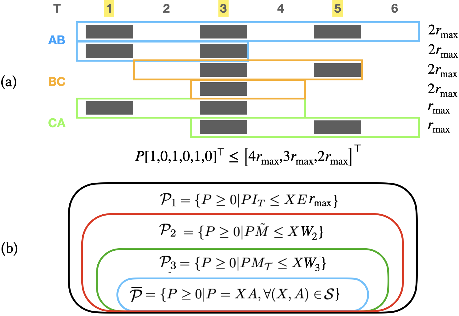
Define $M(m,T)\in\{0,1\}^{n\times{T\choose m}}$ a binary $(m,T)$-selection matrix if all column vectors of $M(m,T)$ form all possible combinations of selecting $m$ out of $T$ entries. If the $i$-th entry is selected by the $j$-th column, $M_{(i,j)}(m,T)=1$ and $M_{(i,j)}(m,T)=0$ otherwise. A binary $(m,T)$-selection matrix is used to represent the aggregated phase power for time steps in $\mathcal{T}$. For instance, as shown in Figure 3(a) with $T=6$, a charging constraint of $P$ can be described with a column vector $[1,0,1,0,1,0]^{\top}$ of $M(3,6)$. Similarly, for all $m\in\mathcal{T}$, we will use every column of $M(m,T)$ to describe a charging constraint in the optimization (9a)-(9). Denote the concatenation of $M(m,T)$ by $M_{\mathcal{T}}$:

Moreover, define $2^{T}-1$ horizontal concatenations of power demand vector $D^{(3)}(\Delta_{T}^{-1})$ as $V\in\mathbb{R}^{N\times 2^{T}-1}$ such that $V\vcentcolon=[D^{(3)}(\Delta_{T}^{-1})|\cdots|D^{(3)}(\Delta_{T}^{-1})]$. Denote $C=\min\{A,B\}$ as the minimum-element operation on two matrices $A$ and $B$, e.g., for any $i,j,C_{(i,j)}=\min\{A_{(i,j)},B_{(i,j)}\}$. Now we can define a set of $P$ as

so that the aggregated power must be bounded by both the sum of chargers’ maximum rates and the total energy demand of EVs that exist in the selected time steps.

Despite that characterizing the constraint (9c) with $P\in\mathcal{P}_{3}$ forms an acceptable relaxed constraint as it considers both the charger’s maximum rate and the EVs’ energy demands, $M_{\mathcal{T}}$ has exponentially many ($2^{T}-1$) columns so that $P\in\mathcal{C}_{p}$ contains more than $2^{T}-1$ linear constraints. To reduce the number of constraints, we can carefully select $m\ll 2^{T}-1$ columns of $M_{\mathcal{T}}$ to form a relaxation of Constraint 9c. In our experiments, we set $\tilde{M}\vcentcolon=\left[I|E^{T}|\mathbf{1}_{T\times 1}\right]$ ($m=T+N+1$) and its corresponding $W_{2}$ as a sub-matrix of $W_{3}$ by selecting the corresponding columns in $W_{3}$. Figure 3 (b) shows the relation of the feasible sets with different choices of $M$ and $W$. Although we cannot guarantee $X\in\mathcal{X}^{*}$ by using $\tilde{M}$, we demonstrate in Section VI the result given by the PXA algorithm using $\tilde{M}$ generates a near-optimal solution. Moreover, in the next section, we prove that in the zero laxity case, considering the relaxation $\mathcal{P}_{1}$ shown in Figure 3(b), solving the optimization (9a)-(9) by setting $M=I_{T}$ and $W=Er_{\max}$ gives an optimal $X^{*}\in\mathcal{X}^{*}$.

Consider the case when all EV sessions have zero laxity, i.e., $\Delta_{T}r_{\max}d_{i}=D_{(i)}$, for any $i\in\mathcal{N}$. Note that the zero-laxity case frequently occurs in specific environments, e.g., fast-charging service centers in roadside rest areas or shopping plazas, wherein most EV drivers leave upon or before their EVs complete charging, thus making EV charging sessions almost zero-laxity. Denote by $I_{T}$ a $T\times T$ identity matrix. The following theorem holds.

Theorem V.1 shows that solving the optimization (9a)-(9) gives an exact $X\in\mathcal{X}^{*}$ in the zero-laxity charging scenarios, thus solving the optimization (8a)-(8d). The following theorem shows that solving the optimization (9a)-(9) by the branch-and-bound method guarantees the convergence to a global optimum with a mild condition $p^{*}_{1}\Delta_{T}=-\sum^{N}_{i=0}D_{(i,3)}$ that ensures the feasibility of EVs’ energy demands.

We use CVXPY [18] for modelling the optimization. GUROBI [19] is used as the branch-and-bound solver for the optimization (9a)-(9), and ECOS [20] for solving the SOCP. We use the ACN-data [6], which is a dataset collected from a real-world ACN at Caltech. The values of ACN parameters in $\mathsf{ACN}=\{D,\mathcal{C}_{\mathrm{r}},\mathcal{C}_{\mathrm{d}},\mathcal{C}_{\mathrm{soc}}\}$ are summarized in Table I. We use $M=\tilde{M}$ and $W=W_{2}$ defined in Section V-A in our experiments. We split EV sessions overnight and treat all EV sessions in one day as a charging episode. The charging data $D$ is selected in the pre-COVID period, from date 2018 May. 1st to 2018 Jul. 31st ($91$ episodes in total).

We consider four benchmarks. (1) (EV RDM.) The phases decided by the incoming EV drivers as in the ACN database. (2) (UNI. RDM.) We draw each phase connection uniformly at random from $\{ab,bc,ca\}$. (3) (RRB. RDM.) We apply the round-robin method based on the arrival time. (4) (WST.) The most unbalanced phase selection by allocating all sessions to one phase line. (5) (M.C.S.A.) The Markov chain simulated annealing method introduced in Section III-B2 with $10000$ iterations per day.

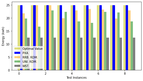
We implement the PXA algorithm in Algorithm 1 for $9$ toy charging scenarios with $T=12$. The first $4$ scenarios are zero-laxity charging (see Section V-B), and the rest are non-zero laxity charging scenarios. Knowing the ACN parameters $\mathsf{ACN}=\{D,\mathcal{C}_{\mathrm{r}},\mathcal{C}_{\mathrm{d}},\mathcal{C}_{\mathrm{soc}}\}$, the PXA algorithm always satisfies $100\%$ of the energy demands, as shown in Figure 4 (a). The uncharged energy demands for WST., UNI. RDM., RRB. RDM. are $50\%$, $19.1\%$ and $9.2\%$ respectively.

We implement the PXA-MPC (Algorithm 2) with the quick-charge function defined in Section II-C and assume the controller only gets to know charging sessions when their arrival times are no $\Delta_{T}$ larger than the current time $t$. In Figure 4 (b), regarding the online performance (solid), the PXA-MPC algorithm charges an additional $7.52\%$ of weekly total energy demand compared against the EV RDM.; $2.86\%$ compared against the UNI.RDM and $1.34\%$ compared against the RRB. RDM.. Offline performance (dashed) is also considered. In particular, we observe that the PXA-MPC algorithm is near-optimal. Moreover, the PXA-MPC takes on average $343.52$ ms to compute at each time step with a standard deviation of $120.42$ ms. In Figure 5 (a), we see the EV RDM. (top) induces an unbalanced three-phase energy dispatch. While the PXA-MPC algorithm (bottom) allocates the energy equally to each phase, especially when the EV demands are high from $10$ am to $8$ pm. We further demonstrate that the PXA-MPC algorithm is capable of satisfying more energy demands compared with other phase optimization methods. In Figure 5(b), we show the trade-off between the line capacity and demand satisfaction. We observe that with the same line capacity, the PXA-MPC algorithm achieves the highest energy efficiency. In practice, the phases of an ACN can be highly unbalanced, and the WST. corresponds to the most unbalanced case when all energy demands are allocated to a single phase.

Since future information on the energy price is usually unknown, we assume no knowledge of the price vector and use the quick charge function to compute $X^{*}$ instead. We demonstrate how the PXA-MPC algorithm can be used to minimize electricity costs. We fix the line capacity as $\mathcal{C}_{\max}=30$. It can be seen in Figure 6, the PXA-MPC satisfies $99.86\%$ of the energy demand, while the EV RDM., UNI. RDM. and the RRB. RDM. meet $96.29\%$, $98.85\%$ and $99.51\%$ respectively. Furthermore, the average electricity price of the PXA-MPC algorithm is $33.85$ cents per kWh, which is constantly lower than that of the EV RDM. ($35$ cents/kWh), the UNI. RDM. ($34.3$ cents/kWh), and the RRB. RDM. ($34.09$ cents/kWh). Compared with the M.C.S.A, the PXA-MPC tends to satisfy higher charging demand in lieu of saving more costs. The phase selection matrix $X^{*}$ computed from the quick charge function helps the PXA-MPC satisfy a higher charging demand than that of the M.C.S.A. In conclusion, the PXA-MPC serves more but costs less compared with other online methods.

References

- [1] J. Zhao, X. Liu, C. Lin, and W. Wei, “Three-phase unbalanced voltage/var optimization for active distribution networks,” in 2016 IEEE Power and Energy Society General Meeting (PESGM), pp. 1–5, 2016.
- [2] H. Khodr, I. Zerpa, P. De Oliveira-De Jesus, and M. Matos, “Optimal phase balancing in distribution system using mixed-integer linear programming,” pp. 1 – 5, 09 2006.
- [3] L. Araujo, D. Penido, S. Carneiro, and J. Pereira, “A three-phase optimal power-flow algorithm to mitigate voltage unbalance,” Power Delivery, IEEE Transactions on, vol. 28, pp. 2394–2402, 10 2013.
- [4] B. Feron, “Why phase optimization matters,” Apr 2021.
- [5] Z. J. Lee, D. Chang, C. Jin, G. S. Lee, R. Lee, T. Lee, and S. H. Low, “Large-scale adaptive electric vehicle charging,” in 2018 IEEE Global Conference on Signal and Information Processing (GlobalSIP), pp. 863–864, 2018.
- [6] Z. J. Lee, T. Li, and S. H. Low, “Acn-data: Analysis and applications of an open ev charging dataset,” in Proceedings of the Tenth ACM International Conference on Future Energy Systems, e-Energy ’19, (New York, NY, USA), p. 139–149, Association for Computing Machinery, 2019.
- [7] Z. J. Lee, S. Sharma, D. Johansson, and S. H. Low, “Acn-sim: An open-source simulator for data-driven electric vehicle charging research,” 2021.
- [8] S. Weckx and J. Driesen, “Load balancing with ev chargers and pv inverters in unbalanced distribution grids,” Sustainable Energy, IEEE Transactions on, vol. 6, pp. 635–643, 04 2015.
- [9] G. Lee, T. Lee, Z. Low, S. H. Low, and C. Ortega, “Adaptive charging network for electric vehicles,” in 2016 IEEE Global Conference on Signal and Information Processing (GlobalSIP), pp. 891–895, 2016.
- [10] L. Guo, K. F. Erliksson, and S. H. Low, “Optimal online adaptive electric vehicle charging,” in 2017 IEEE Power Energy Society General Meeting, pp. 1–5, 2017.
- [11] Z. J. Lee, G. Lee, T. Lee, C. Jin, R. Lee, Z. Low, D. Chang, C. Ortega, and S. H. Low, “Adaptive charging networks: A framework for smart electric vehicle charging,” 2020.
- [12] T. Li, B. Sun, Y. Chen, Z. Ye, S. H. Low, and A. Wierman, “Learning-based predictive control via real-time aggregate flexibility,” IEEE Transactions on Smart Grid, vol. 12, no. 6, pp. 4897–4913, 2021.
- [13] Y. Hu, S. Su, L. He, X. Wu, T. Ma, Z. Liu, and X. Wei, “A real-time multilevel energy management strategy for electric vehicle charging in a smart electric energy distribution system,” Energy Technology, vol. 7, no. 5, p. 1800705, 2019.
- [14] A. Hernández-Arauzo, J. Puente Peinador, R. Arias, and J. Sedano, “Electric vehicle charging under power and balance constraints as dynamic scheduling,” Computers and Industrial Engineering, vol. 85, 04 2015.
- [15] F. Shahnia, A. Ghosh, G. Ledwich, and F. Zare, “Predicting voltage unbalance impacts of plug-in electric vehicles penetration in residential low-voltage distribution networks,” Electric Power Components and Systems, vol. 41, no. 16, pp. 1594–1616, 2013.
- [16] A. Rezai and S. Elham, “Grid-able plug-in electric vehicles in smart grids: Incorporation into demand response,” 2016.
- [17] Y.-J. Kuo and H. D. Mittelmann, “Interior point methods for second-order cone programming and or applications,” Computational Optimization and Applications, vol. 28, pp. 255–285, Sep 2004.
- [18] S. Diamond and S. Boyd, “CVXPY: A Python-embedded modeling language for convex optimization,” Journal of Machine Learning Research, vol. 17, no. 83, pp. 1–5, 2016.
- [19] Gurobi Optimization, LLC, “Gurobi Optimizer Reference Manual,” 2021.
- [20] A. Domahidi, E. Chu, and S. Boyd, “Ecos: An socp solver for embedded systems,” in 2013 European Control Conference (ECC), pp. 3071–3076, IEEE, 2013.