Hot-spots Detection in Count Data by Poisson Assisted Smooth Sparse Tensor Decomposition

In this subsection, we review the existing literature on hot-spots detection based on three types of count data: univariate, multivariate, and multivariate spatio-temporal.

For univariate count data, i.e., when we observe the data of the form $\{y_{t}\}_{t=1,\ldots,T}$ with $y_{t}\in\mathbbm{N}$ (a set of non-negative integers) denoting the observed count data at time $t$, there are mainly four methods to detect hot-spots: (1) time series based method [22, see]; (2) control charts based method by using the likelihood functions, such as the cumulative sum (CUSUM) control chart [16, see] and exponentially weighted moving average (EWMA) control chart [16, see]; (3) scan statistics based method [28, see], including both the frequentist scan statistics [29, see] and Bayesian scan statistics [34, see]; (4) Poisson process-based method that is often combined with Bayesian methods [21, see].

For multivariate count data, i.e., when we observe the data of the form $\{y_{it}\}_{i=1,\ldots,n,t=1,\ldots,T}$ with $y_{it}\in\mathbbm{N}$, there are mainly three methods widely-used hot-spots detection: (1) control chart based method, including CUSUM or EWMA control charts [30, see]; (2) Poisson process based method [44, see]; (3) hidden Markov model (HMM) based method [9, see].

For multivariate spatio-temporal count data, i.e., when the observed data are of the form $y_{ijt}\in\mathbbm{N}$ that denotes the observed count data over the $i$-th spatial location for the $j$-th type of disease at time $t$ with $i=1,\ldots,n_{1},j=1,\ldots,n_{2},t=1,\ldots,T$, research on hot-spots detection is rather limited, although there are three types of closely related methods developed for other purposes or other contexts: (1) scan statistics for anomalous clusters, (2) tensor decomposition for Gaussian data, and (3) change point detection for global changes. Since our paper deals with multivariate spatio-temporal count data, below we will provide a more detailed review of these three methods.

For the scan statistics based method, it was first developed in the 1960s [33, see] and later extended by [26] to detect anomalous clusters in spatio-temporal data. The main idea of scan statistics is to detect the abnormal clusters by utilizing a maximal log-likelihood ratio. It is worth noting that the scan statistics-based method is a parametric method that assumes the data distributions are known. For instance, authors of [42] assumes the negative binomial distribution, [27] investigate the Poisson distribution. A limitation of the scan statistics is that it assumes that the background is independent and identically distributed (i.i.d.) or follows a rather simple probability distribution, which might not be suitable to handle non-stationary spatio-temporal data.

For the tensor decomposition-based detection, one representative is [48] for Gaussian data, and below is the main idea. First, it assumes that the raw data follows the normal distribution and then decomposes it into three components: global trend mean, local hot-spots, and residuals. Then, it uses the Tucker decomposition [19, see] to decompose the first two components. Finally, it detects the hot-spots by monitoring the model residuals. Similar ideas can also be found in elsewhere, for example, [47]. The limitation of this method is that it does not consider the effect of population size and the normal distribution is clearly inappropriate for count data, especially those small values. Another representative is [12], where the authors first assume the count data follows the Poisson distribution and then decompose the Poisson mean by canonical polyadic decomposition (CPD) [19, see], and finally localize the hot-spots by small p-values. The limitation of this approach is that it does not remove the global trend mean from the raw data, which leads to its incapacity to detect the local hot-spots. Besides, it can only realize the hot-spots localization, and the analysis of the detection delay is not reported.

For the change-point detection framework, there are two related categories, the Least Absolute Shrinkage and Selection (Lasso) based methods and dimension reduction based methods. For the Lasso-based change-point detection method, one of the existing research representative is [55]. Note that Lasso has been demonstrated to be an effective method for variable selection to address sparsity issues for high-dimensional data in the past decades since its developments in [43], and thus it is natural to apply it to detect sparse changes in high-dimensional data [45, 55, 56, 52, see]. While the sparse change of Lasso is similar to the hot-spots, unfortunately, as our extensive simulation studies will demonstrate, the Lasso-based control chart is unable to separate the local hot-spots from the non-stationary global trend mean in the spatio-temporal data. For the dimension reduction-based method, the representative is [11]. The main idea of this type of method is that it first uses principal component analysis (PCA) or other dimension reduction methods to extract the features from the high-dimensional data, and then it combines the reduced dimension information with change-point models to detect the hot-spots. For other dimension-reduction-methods, please see [37, 11, 7] for more details. The drawbacks of the dimension reduction-based method are the restriction of the change-point detection problem and the failure to consider the spatial sparsity and temporal consistency of hot-spots.

The essential idea of our proposed method is to combine the tensor decomposition-based method and the Lasso-based method over the multivariate spatio-temporal data. Mathematically speaking, the multivariate spatio-temporal data can be a tensor of order three, which is a multi-dimensional array, i.e., $\mathcal{Y}\in\mathbb{R}^{n_{1}\times n_{2}\times n_{3}}$. Here $n_{1}$ is the number of the spatial locations, $n_{2}$ is the number of different diseases or variates, and $n_{3}$ is the number of time points. In our proposed method, we assume the tensor $\mathcal{Y}$ comes from the Poisson distribution and then consider the additive model that decomposes its Poisson rate into two components: (1) smooth but non-stationary global trend mean, and (2) sparse local hot-spots. Next, we fit the raw data with a penalty function, i.e., a Lasso type penalty to guarantee the spatial sparsity of hot-spots. This allows us to not only detect when the hot-spots happen over the temporal domain (i.e., hot-spots detection problem) but also localize where and which types/attributes of the hot-spots occur if the change happens (i.e., hot-spots localization problem). We term our proposed decomposition method as Poisson-assisted Smooth Sparse Tensor Decomposition (PoSSTenD).

It is useful to highlight the novelty of our proposed method as compared to those existing methods on multivariate spatio-temporal count data. First, our proposed PoSSTenD method takes into account of the effect of population size to focus on the anomalous infectious diseases rates or Poisson rates, which is important in many real-world applications. Second, our proposed PoSSTenD method can detect hot-spots when the global trend of the spatio-temporal data is dynamic (i.e., non-stationary or non-i.i.d). That is, our method is robust no matter whether the global trend is decreasing, stationary, or increasing, in the sense that it can detect hot-spots with positive or negative local mean shifts on top of the global trend of raw data. In comparison, existing SPC or change-point detection methods often assume that the background is i.i.d. and focus on detecting the anomalies under the static and i.i.d. background. Finally, while our paper focuses only on the tensor of order three arising from our motivating application in 10 annual infectious diseases in the U.S., our proposed hot-spots method can easily be extended to the tensor of order $d$ ($d\geq 3$), as we can simply add corresponding dimensions and bases in the tensor analysis. The capability of extending to high-dimensional tensor data is one of the main advantages of our proposed PoSSTenD method.

We would like to clarify that our contribution lies in the hot-spots detection and localization, instead of model fitting/prediction of the multivariate spatio-temporal count data. For the fitness of the count data, there are lots of well-established methods. One widely used one is the generalized linear regression model [see 17, Chapter 3]. Another popular method is the time series models such as Autoregressive Moving Average (ARMA).In this paper, we will not compare our proposed PoSSTenD method to these methods, because our objective is to detect and localize hot-spots, rather than model fitting.

The remainder of this paper is as follows. In Section 2, we introduce and visualize a motivating dataset. In Section 3, we present our proposed PoSSTenD method, discuss how to estimate model parameters from data, and describe how to use our proposed PoSSTenD method to detect and localize hot-spots. Our proposed method is compared with several benchmark methods in Section 4, demonstrating its usefulness through extensive simulations. The application of our proposed method in the dataset (described in Section 2) is reported in Section 2.

Our motivated data are from CDC on the number of annual new cases infected by 10 different diseases of 49 mainland US states from 1993 to 2018. The 10 infectious diseases are (1) mumps, (2) legionellosis, (3) tuberculosis, (4) syphilis, (5) shigellosis, (6) pertussis, (7) hepatitis A, (8) hepatitis B, (9) rabies, (10) malaria. The dataset is publicly available in https://www.cdc.gov/mmwr/mmwr_nd/index.html (for data from 1993 to 2015) and https://wonder.cdc.gov/nndss/nndss_annual_tables_menu.asp (for data from 2016-2018). For illustration, we present the a selected subset of this dataset in Table 1, where the states are listed in alphabetical order.

Mathematically, we can organize the above motivating dataset into a tensor of order three, i.e., $\mathcal{Y}\in\mathbb{R}^{n_{1}\times n_{2}\times n_{3}}$, where $n_{1}=49$ is the number of states, $n_{2}=10$ is the number of diseases, and $n_{3}=26$ is the number of observed years. For this tensor of order three $\mathcal{Y}$, its $(i,j,t)$-th entry, i.e., $\mathcal{Y}_{i,j,t}$ is the number of people get infected by the $j$-th type of disease in the $i$-th state $i$ in year $t$.

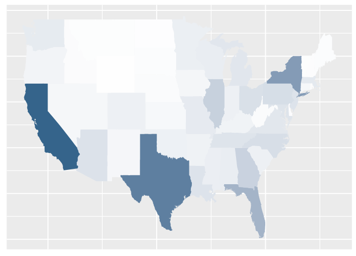
To better capture the character of the data $\mathcal{Y}$, we provide some data visualization plots in Figure 1. In Figure 1(a), we show the bar plot for the total number of affected subjects for these ten different diseases. Here the $j$-th bar represents the $j$-th type of disease and the height of $j$-th bar is the value of $\sum_{i=1}^{n_{1}}\sum_{t=1}^{n_{3}}\mathcal{Y}_{i,j,t}.$ In Figure 1(b), we plot the cumulative number of infected subjects of 49 states in a map, where the color of the $i$-th state is decided by the total value $\sum_{j=1}^{n_{2}}\sum_{t=1}^{n_{3}}\mathcal{Y}_{i,j,t}$ and a larger value leads to a deeper color. From this plot, we find that generally speaking, California, Texas, and New York observe a larger number of infected subjects as compared with other states, possibly due to a large population size. In Figure 1(c), we display a time series plot, where the x-axis is the year and the y-axis is the logarithm of the value of $\sum_{i=1}^{n_{1}}\sum_{j=1}^{n_{2}}\mathcal{Y}_{i,j,t}$ for $t=1,2,\ldots,n_{3}$. We can see that, there is a trough from 2000 to 2010, but the number of infected people has an increasing trend otherwise.

In this subsection, we present necessary tensor notations and tensor algebra so as to help readers understand our proposed methodology in Section 3.

First, for the notations throughout the paper, scalars are denoted by lowercase letters (e.g., $\theta,y$), and vectors are denoted by lowercase boldface letters ($\boldsymbol{\theta},\mathbf{y}$), whose $i$-th entry is denoted by the subscript ($\boldsymbol{\theta}_{i},\mathbf{y}_{i}$). Matrices are denoted by uppercase boldface letter ($\boldsymbol{\Theta},\mathbf{Y}$), whose $(i,j)$-th entry is denoted by the subscript ($\boldsymbol{\Theta}_{i,j},\mathbf{Y}_{ij}$). Tensors are denoted by curlicue letter ($\vartheta,\mathcal{Y}$). For example, an $K$-dimension tensor is represented by $\vartheta\in\mathbb{R}^{I_{1}\times\ldots\times I_{K}},$ where $I_{k}$ represent the mode-$K$ dimension of $\vartheta$ for $k=1,\ldots,K$. Its $(i_{1},i_{2},\ldots,i_{K})$-th entry is denoted by the subscript ($\vartheta_{i_{1},i_{2},\ldots,i_{K}},\mathcal{Y}_{i_{1},i_{2},\ldots,i_{K}}$).

Next, we introduce the definition of slice in tensor. The slice is a two-dimensional section of a tensor by fixing all but two indices. Let us take a 3-dimension tensor $\mathcal{Y}\in\mathbb{R}^{n_{1}\times n_{2}\times n_{3}}$ as an example. Its horizontal, lateral, and frontal slides are denoted by $\mathcal{Y}_{i::}(\forall i=1,\ldots,n_{1}),\mathcal{Y}_{:j:}(\forall j=1,\ldots,n_{2}),$ and $\mathcal{Y}_{::t}\;(\forall t=1,\ldots,n_{3}),$ respectively. A visualization of the aforementioned three types of slides are available in Figure 3 of [53].

Finally, we introduce the Tucker decomposition. It can be regarded as an extension of singular value decomposition (SVD) in the matrix. Mathematically, it decomposes a tensor $\mathcal{Y}\in\mathbb{R}^{n_{1}\times n_{2}\times\ldots\times n_{d}}$ into a product of a “core tensor” $\mathcal{C}$ and several matrices $\mathbf{B}_{1},\ldots,\mathbf{B}_{d}$ which correspond to different core scalings along each mode, i.e.,

where $\times_{n}$ is the mode-n product for any $n=1,\ldots,d$ [see 53, Section 2]. And the core tensor $\mathcal{C}$ is of dimension $\mathcal{C}\in\mathbb{R}^{p_{1}\times p_{2}\times\ldots\times p_{d}}$. The matrix $\mathbf{B}_{i}$ is of dimension $\mathbf{B}_{i}\in\mathbb{R}^{n_{i}\times p_{i}}$ for any $i=1,\ldots,d$. In most of the applications, we assume the matrices $\mathbf{B}_{1},\ldots,\mathbf{B}_{d}$ are known [49, 47, 46, see]. The high-level criterion to select $\mathbf{B}_{1},\ldots,\mathbf{B}_{d}$ are listed as follows. If the data $\mathcal{Y}$ has a smooth pattern on mode-n, then one can use the either spline basis [49, 15, see] or Gaussian kernel [49, see] for $\mathbf{B}_{n}$. If the data $\mathcal{Y}$ has no prior information on mode-n, then one can use the identity matrix for $\mathbf{B}_{n}$ [53, see]. And we call $\min\{p_{1},p_{2},\ldots,p_{d}\}$ as the rank of the Tucker decomposition [24, see].

In this subsection, we present the mathematical model of our proposed PoSSTenD method. For better illustration, we take the motivating dataset described in Section 2 as an example, which is a tensor of order three, i.e., $\mathcal{Y}\in\mathbb{R}^{n_{1}\times n_{2}\times n_{3}}$. The $(i,j,t)$-th entry of $\mathcal{Y}$ is the number of people who are infected by the $j$-th type of disease in the $i$-th state in year $t$. Since the number of infected patients is count data, we assume that it follows the Poisson distribution:

where $\mathcal{R}_{i,j,t}$ is the infectious rate of the $j$-th type of disease in the $i$-th state in year $t$, and $\mathcal{N}_{i,j,t}$ denotes the corresponding population size, for $i=1\ldots n_{1},j=1\ldots n_{2},t=1\ldots n_{3}$. In our simulation studies and case study, we assume that the population size $\mathcal{N}_{i,j,t}$ is the same over different disease type $j$, although they can be different under other scenarios, e.g., when certain diseases will affect certain sub-populations depending on gender, age, race, etc.

In our paper, we are interested in detecting and localizing the hot-spots in infectious rate $\mathcal{R}_{i,j,t}$, and thus we further decomposed the logarithm of the infectious rates into two components: the smooth global trend mean $\mathcal{U}_{i,j,t}$ and the local hot-spots $\mathcal{H}_{i,j,t}$. Mathematically, it is an additive model:

where $\mathcal{U}_{i,j,t}$ and $\mathcal{H}_{i,j,t}$ are the $(i,j,t)$-th entry of tensors $\mathcal{U}$ and $\mathcal{H}\in\mathbb{R}^{n_{1}\times n_{2}\times n_{3}},$ respectively.

For the first component – the global trend mean $\mathcal{U}\in\mathbb{R}^{n_{1}\times n_{2}\times n_{3}}$ – we apply Tucker decomposition for dimension reduction of tensors, i.e.,

where $\mathbf{B}_{m,1}\in\mathbb{R}^{n_{1}\times p_{1}},\mathbf{B}_{m,2}\in\mathbb{R}^{n_{2}\times p_{2}},\mathbf{B}_{m,3}\in\mathbb{R}^{n_{3}\times p_{3}}$ are the pre-assigned basis describing the within-state correlation, within-disease-type correlation, and within-year correlation in $\mathcal{U}$, respectively. For the selection of $\mathbf{B}_{m,1},\mathbf{B}_{m,2},\mathbf{B}_{m,3}$, we postpone its discussion at the end of this subsection. The operators $\times_{1},\times_{2},\times_{3}$ are the mode-$n$ product reviewed in Section 2.2 with $n=1,2,3$. These three mode-$n$ products are used to model the between-dimension correlations in $\mathcal{U}$. The tensor $\vartheta_{m}\in\mathbb{R}^{p_{1}\times p_{2}\times p_{3}}$ is an unknown tensor parameter to be estimated.

For the second component – local hot-spots $\mathcal{H}\in\mathbb{R}^{n_{1}\times n_{2}\times n_{3}}$ – we apply the similar Tucker decomposition as in $\mathcal{U}$:

where the $\vartheta_{h}\in\mathbb{R}^{q_{1}\times q_{2}\times q_{3}}$ is the unknown parameter to be estimated and basis $\mathbf{B}_{h,1}\in\mathbb{R}^{n_{1}\times q_{1}},\mathbf{B}_{h,2}\in\mathbb{R}^{n_{2}\times q_{2}},\mathbf{B}_{h,3}\in\mathbb{R}^{n_{3}\times q_{3}}$ are pre-assigned matrices describing the within-state correlation, within-disease-type correlation, and within-year correlation in $\mathcal{H}$, respectively. The suitable choices of these bases will be discussed in more details in Section 4. The operators $\times_{1},\times_{2},\times_{3}$ are the mode-$n$ product used to model the between-dimension correlations in $\mathcal{H}$.

By combining (1), (2), (3), (4), we summarize our method as

where $(\vartheta_{m}\times_{1}\mathbf{B}_{m,1}\times_{2}\mathbf{B}_{m,2}\times_{3}\mathbf{B}_{m,3})_{i,j,t},(\vartheta_{h}\times_{1}\mathbf{B}_{h,1}\times_{2}\mathbf{B}_{h,2}\times_{3}\mathbf{B}_{h,3})_{i,j,t}$ denote the $(i,j,t)$-th entry in tensor $\vartheta_{m}\times_{1}\mathbf{B}_{m,1}\times_{2}\mathbf{B}_{m,2}\times_{3}\mathbf{B}_{m,3},\vartheta_{h}\times_{1}\mathbf{B}_{h,1}\times_{2}\mathbf{B}_{h,2}\times_{3}\mathbf{B}_{h,3}\in\mathbb{R}^{n_{1}\times n_{2}\times n_{3}},$ respectively.

This tensor representation allows us to develop computationally efficient methods for estimation and prediction. Under tensor algebra, the above model can be rewritten as

Here vectors $\mathbf{y},\mathbf{r},\mathbf{n}\in\mathbb{R}^{n_{1}n_{2}n_{3}},\boldsymbol{\theta}_{m}\in\mathbb{R}^{p_{1}p_{2}p_{3}},\boldsymbol{\theta}_{h}\in\mathbb{R}^{q_{1}q_{2}q_{3}}$ are the vectorized form of tensor $\mathcal{Y},\mathcal{R},\mathcal{N}\in\mathbb{R}^{n_{1}\times n_{2}\times n_{3}},\vartheta_{m}\in\mathbb{R}^{p_{1}\times p_{2}\times p_{3}},\vartheta_{h}\in\mathbb{R}^{q_{1}\times q_{2}\times q_{3}},$ respectively. The operator $\odot$ is the Hadamard product, i.e., the output of $\mathbf{r}\odot\mathbf{n}$ is a vector of length $n_{1}n_{2}n_{3}$, whose $i$-th entry is $r_{i}\times n_{i}$ with $r_{i},n_{i}$ as the $i$-th elements of vector $\mathbf{r},\mathbf{n}$, respectively. The operator $\otimes$ is the Kronecker product whose mathematical definition can be found in [53, 50]. Besides, the operator $\dot{\sim}$ means that the $i$-th entry of $\mathbf{y}$ follows the Poisson distribution with parameter $r_{i}n_{i}$ for any $i=1,\ldots,n_{1}n_{2}n_{3}$.

In the reminder of this subsection, we articulate the selection of basis for global trend mean $\mathbf{B}_{m,1},\mathbf{B}_{m,2},\mathbf{B}_{m,3}$, and basis for local hot-spots $\mathbf{B}_{h,1},\mathbf{B}_{h,2},\mathbf{B}_{h,3}$, particularly in our case study.

For the selection of $\mathbf{B}_{m,1},\mathbf{B}_{m,2},\mathbf{B}_{m,3}$, given $\mathcal{Y}$’s smooth pattern, we use the cubic B-spline basis with 8, 7, 7 knots in the x-direction (spatial domain), y-direction (disease-categorical domain) and z-direction (temporal domain). This selection strategy is also adopted in Section 6 of [49], and the above three sets of knots are reasonable in our case study. In general, a smaller number of knots may result in the loss of detection accuracy, and a larger number of knots will lead to the selection of normal regions with large noises. As pointed out by [41], as long as the number of knots is sufficiently large to capture the variation of the background, a further increase in knots will have little effect due to the regulation of smoothness. After verifying the above three sets of knots by generalized cross validation (GCV), as suggested by [41], we find they are sufficient large to capture the variation of the global trend mean. Other choice of $\mathbf{B}_{m,1},\mathbf{B}_{m,2},\mathbf{B}_{m,3}$ is welcomed, for example, the Gaussian kernel basis [53, 49, see]. In this paper, we will use the B-spline basis for illustration of our proposed PoSSTenD method. Given the above selection of $\mathbf{B}_{m,1},\mathbf{B}_{m,2},\mathbf{B}_{m,3}$, the rank of the Tucker decomposition of $\mathcal{U}$ is $\min\{p_{1},p_{2},p_{3}\}=4$.

For the selection of $\mathbf{B}_{h,1},\mathbf{B}_{h,2},\mathbf{B}_{h,3}$, we set them as the identity matrices, due to the following two reasons. First, there is no prior information about the hot-spots distribution, which makes identity matrices a reasonable choice. Second, we aim at detecting sparse hot-spots. If one in interested in detecting clustered hot-spots, then a spline basis is a better choice [see 47, Section 3.4]. Given the above selection of $\mathbf{B}_{h,1},\mathbf{B}_{h,2},\mathbf{B}_{h,3}$, the rank of the Tucker decomposition of $\mathcal{H}$ is $\min\{n_{1},n_{2},n_{3}\}=10$ in the our case. This rank is not reduced much, because we do not want to lose much information considering the hot-spots detection accuracy.

This subsection discusses the parameter estimation of our proposed PoSSTenD method. We will first formulate the parameter estimation as an optimization problem in Subsection 3.2.1, and then develop an efficient algorithm to solve this optimization problem in Subsection 3.2.2.

In this subsection, we discuss the detection and localization of the hot-spots. For the ease of presentation, we first discuss the hot-spots detection, i.e., detect when a hot-spot occurs in Subsection 3.3.1. Then, in Subsection 3.3.2, we consider the localization of the hot-spots, i.e., determine which states and which type of diseases are involved for the detected hot-spots.

References

- Beck and Teboulle, [2009] Beck, A. and Teboulle, M. (2009). A fast iterative shrinkage-thresholding algorithm for linear inverse problems. SIAM journal on imaging sciences, 2(1):183–202.
- Brègman, [1966] Brègman, L. M. (1966). Relaxation method for finding a common point of convex sets and its application to optimization problems. In Doklady Akademii Nauk, volume 171, pages 1019–1022. Russian Academy of Sciences.
- Chen and Fang, [2019] Chen, J. and Fang, F. (2019). Semiparametric likelihood for estimating equations with non-ignorable non-response by non-response instrument. Journal of Nonparametric Statistics, 31(2):420–434.
- [4] Chen, J., Fang, F., and Xiao, Z. (2018a). Semiparametric inference for estimating equations with nonignorably missing covariates. Journal of Nonparametric Statistics, 30(3):796–812.
- [5] Chen, J., Ohlssen, D., and Zhou, Y. (2018b). Functional mixed effects model for the analysis of dose-titration studies. Statistics in Biopharmaceutical Research, 10(3):176–184.
- [6] Chen, J., Shao, J., and Fang, F. (2021a). Instrument search in pseudo-likelihood approach for nonignorable nonresponse. Annals of the Institute of Statistical Mathematics, 73(3):519–533.
- [7] Chen, J., Xie, B., and Shao, J. (2018c). Pseudo likelihood and dimension reduction for data with nonignorable nonresponse. Statistical Theory and Related Fields, 2(2):196–205.
- [8] Chen, Q., Chen, J., Zhou, Y., Huang, L., Tang, Y., Li, J., and Zhang, J. (2021b). Natural history and associated early life factors of childhood asthma: a population registry-based cohort study in denmark. BMJ open, 11(11):e045728.
- Conesa et al., [2015] Conesa, D., Martínez-Beneito, M., Amorós, R., and López-Quílez, A. (2015). Bayesian hierarchical poisson models with a hidden markov structure for the detection of influenza epidemic outbreaks. Statistical methods in medical research, 24(2):206–223.
- Daubechies et al., [2004] Daubechies, I., Defrise, M., and De Mol, C. (2004). An iterative thresholding algorithm for linear inverse problems with a sparsity constraint. Communications on Pure and Applied Mathematics: A Journal Issued by the Courant Institute of Mathematical Sciences, 57(11):1413–1457.
- De Ketelaere et al., [2015] De Ketelaere, B., Hubert, M., and Schmitt, E. (2015). Overview of PCA-based statistical process-monitoring methods for time-dependent, high-dimensional data. Journal of Quality Technology, 47(4):318–335.
- Eren et al., [2020] Eren, M. E., Moore, J. S., and Alexandro, B. S. (2020). Multi-dimensional anomalous entity detection via poisson tensor factorization. In 2020 IEEE International Conference on Intelligence and Security Informatics (ISI), pages 1–6. IEEE.
- Friedman et al., [2010] Friedman, J., Hastie, T., and Tibshirani, R. (2010). Regularization paths for generalized linear models via coordinate descent. Journal of statistical software, 33(1):1.
- Friedman et al., [2001] Friedman, J., Hastie, T., Tibshirani, R., et al. (2001). The elements of statistical learning, volume 1. Springer series in statistics New York.
- Gahrooei et al., [2021] Gahrooei, M. R., Yan, H., Paynabar, K., and Shi, J. (2021). Multiple tensor-on-tensor regression: An approach for modeling processes with heterogeneous sources of data. Technometrics, 63(2):147–159.
- Han et al., [2010] Han, S. W., Tsui, K.-L., Ariyajunya, B., and Kim, S. B. (2010). A comparison of cusum, ewma, and temporal scan statistics for detection of increases in poisson rates. Quality and Reliability Engineering International, 26(3):279–289.
- Hastie et al., [2015] Hastie, T., Tibshirani, R., and Wainwright, M. (2015). Statistical learning with sparsity: the lasso and generalizations. CRC press.
- Hawkins, [1993] Hawkins, D. M. (1993). Regression adjustment for variables in multivariate quality control. Journal of Quality Technology, 25(3):170–182.
- Hitchcock, [1927] Hitchcock, F. L. (1927). The expression of a tensor or a polyadic as a sum of products. Journal of Mathematics and Physics, 6(1-4):164–189.
- Hunyadi, [2020] Hunyadi, L. (2020). B-splines. https://www.mathworks.com/matlabcentral/fileexchange/27374-b-splines.
- Ihler et al., [2006] Ihler, A., Hutchins, J., and Smyth, P. (2006). Adaptive event detection with time-varying poisson processes. In Proceedings of the 12th ACM SIGKDD international conference on Knowledge discovery and data mining, pages 207–216.
- Killick and Eckley, [2014] Killick, R. and Eckley, I. (2014). changepoint: An r package for changepoint analysis. Journal of statistical software, 58(3):1–19.
- Kim and Akritas, [2010] Kim, M. H. and Akritas, M. G. (2010). Order thresholding. The annals of statistics, 38(4):2314–2350.
- Kolda and Bader, [2009] Kolda, T. G. and Bader, B. W. (2009). Tensor decompositions and applications. SIAM review, 51(3):455–500.
- Kullback and Leibler, [1951] Kullback, S. and Leibler, R. A. (1951). On information and sufficiency. The annals of mathematical statistics, 22(1):79–86.
- Kulldorff, [1997] Kulldorff, M. (1997). A spatial scan statistic. Communications in Statistics-Theory and methods, 26(6):1481–1496.
- Kulldorff, [2001] Kulldorff, M. (2001). Prospective time periodic geographical disease surveillance using a scan statistic. Journal of the Royal Statistical Society: Series A (Statistics in Society), 164(1):61–72.
- Kulldorff et al., [2009] Kulldorff, M., Huang, L., and Konty, K. (2009). A scan statistic for continuous data based on the normal probability model. International journal of health geographics, 8(1):1–9.
- Kulldorff and Nagarwalla, [1995] Kulldorff, M. and Nagarwalla, N. (1995). Spatial disease clusters: detection and inference. Statistics in medicine, 14(8):799–810.
- Liu et al., [2019] Liu, K., Zhang, R., and Mei, Y. (2019). Scalable sum-shrinkage schemes for distributed monitoring large-scale data streams. Statistica Sinica, 29(1):1–22.
- Lorden, [1971] Lorden (1971). Procedures for reacting to a change in distribution. The Annals of Mathematical Statistics, 42(6):1897–1908.
- Nagaraja, [1982] Nagaraja, H. (1982). Some nondegenerate limit laws for the selection differential. The Annals of Statistics, pages 1306–1310.
- Naus, [1963] Naus, J. I. (1963). Clustering of random points in line and plane. Harvard University Press.
- Neill et al., [2005] Neill, D., Moore, A., and Cooper, G. (2005). A bayesian spatial scan statistic. Advances in neural information processing systems, 18:1003–1010.
- Neill et al., [2006] Neill, D. B., Moore, A. W., and Cooper, G. F. (2006). A bayesian spatial scan statistic. In Advances in neural information processing systems, pages 1003–1010.
- Page, [1954] Page, E. S. (1954). Continuous inspection schemes. Biometrika, 41(1/2):100–115.
- Paynabar et al., [2013] Paynabar, K., Jin, J., and Pacella, M. (2013). Monitoring and diagnosis of multichannel nonlinear profile variations using uncorrelated multilinear principal component analysis. Iie transactions, 45(11):1235–1247.
- Pinheiro and Bates, [2006] Pinheiro, J. and Bates, D. (2006). Mixed-effects models in S and S-PLUS. Springer Science & Business Media.
- Polson et al., [2015] Polson, N. G., Scott, J. G., Willard, B. T., et al. (2015). Proximal algorithms in statistics and machine learning. Statistical Science, 30(4):559–581.
- Qiu, [2013] Qiu, P. (2013). Introduction to statistical process control. Chapman and Hall/CRC.
- Ruppert, [2002] Ruppert, D. (2002). Selecting the number of knots for penalized splines. Journal of computational and graphical statistics, 11(4):735–757.
- Tango et al., [2011] Tango, T., Takahashi, K., and Kohriyama, K. (2011). A space–time scan statistic for detecting emerging outbreaks. Biometrics, 67(1):106–115.
- Tibshirani, [1996] Tibshirani, R. (1996). Regression shrinkage and selection via the lasso. Journal of the Royal Statistical Society. Series B (Methodological), pages 267–288.
- Turcotte et al., [2016] Turcotte, M., Moore, J., Heard, N., and McPhall, A. (2016). Poisson factorization for peer-based anomaly detection. In 2016 IEEE Conference on Intelligence and Security Informatics (ISI), pages 208–210. IEEE.
- Wei et al., [2018] Wei, S.-b., Wang, W., Liu, N., Chen, J., Guo, X.-y., Tang, R.-b., Yu, R.-h., Long, D.-y., Sang, C.-h., Jiang, C.-x., et al. (2018). U-shaped association between serum free triiodothyronine and recurrence of atrial fibrillation after catheter ablation. Journal of Interventional Cardiac Electrophysiology, 51(3):263–270.
- Yan et al., [2014] Yan, H., Paynabar, K., and Shi, J. (2014). Image-based process monitoring using low-rank tensor decomposition. IEEE Transactions on Automation Science and Engineering, 12(1):216–227.
- Yan et al., [2017] Yan, H., Paynabar, K., and Shi, J. (2017). Anomaly detection in images with smooth background via smooth-sparse decomposition. Technometrics, 59(1):102–114.
- [48] Yan, H., Paynabar, K., and Shi, J. (2018a). Real-time monitoring of high-dimensional functional data streams via spatio-temporal smooth sparse decomposition. Technometrics, 60(2):181–197.
- [49] Yan, H., Paynabar, K., and Shi, J. (2018b). Real-time monitoring of high-dimensional functional data streams via spatio-temporal smooth sparse decomposition. Technometrics, 60(2):181–197.
- Zhao, [2021] Zhao, Y. (2021). New progress in hot-spots detection, partial-differential-equation-based model identification and statistical computation. PhD thesis, Georgia Institute of Technology.
- Zhao and Huo, [2020] Zhao, Y. and Huo, X. (2020). A homotopic method to solve the lasso problems with an improved upper bound of convergence rate. arXiv preprint arXiv:2010.13934.
- [52] Zhao, Y., Huo, X., and Mei, Y. (2021a). Identification of underlying dynamic system from noisy data with splines. arXiv preprint arXiv:2103.10231.
- [53] Zhao, Y., Yan, H., Holte, S., and Mei, Y. (2021b). Rapid detection of hot-spots via tensor decomposition with applications to crime rate data. Journal of Applied Statistics, pages 1–27.
- Zhao et al., [2019] Zhao, Y., Yan, H., Holte, S. E., Kerani, R. P., and Mei, Y. (2019). Rapid detection of hot-spot by tensor decomposition with application to weekly gonorrhea data. In International Workshop on Intelligent Statistical Quality Control, pages 265–286. Springer.
- Zou and Qiu, [2009] Zou, C. and Qiu, P. (2009). Multivariate statistical process control using lasso. Journal of the American Statistical Association, 104(488):1586–1596.
- Zou et al., [2008] Zou, C., Tsung, F., and Wang, Z. (2008). Monitoring profiles based on nonparametric regression methods. Technometrics, 50(4):512–526.
Appendix A Proof for Proposition 3.1
Proof.
According to Newton-Raphson method, we update from to as follows: