跳到论文正文
W Papers独立论文阅读器 arXiv:2205.10398 论文正文 计算阅读时间 · 0%
引用这篇论文根据当前论文元数据生成,正式投稿前建议核对。


License: CC BY 4.0
arXiv:2205.10398v2 [hep-th] 07 Jul 2022

August 11, 2026

Janus and RG interfaces in three-dimensional gauged supergravity II: General α\alpha

Michael Gutperle and Charlie Hultgreen-Mena

Mani L. Bhaumik Institute for Theoretical Physics
Department of Physics and Astronomy
University of California, Los Angeles, CA 90095, USA

Abstract

In this paper, we continue the study of Janus and RG-flow interfaces in three dimensional supergravity continuing the work presented in [1]. We consider 𝒩=8\mathcal{N}=8 gauged supergravity theories which have a 𝒩=(4,4)\mathcal{N}=(4,4) A​d​S3AdS_{3} vacuum with D1​(2,1,α)×D1​(2,1,α)D^{1}(2,1;\alpha)\times D^{1}(2,1;\alpha) symmetry for general α\alpha. We derive the BPS flow equations and find numerical solutions. Some holographic quantities such as the entanglement entropy are calculated.

1 Introduction

Janus solutions provide a holographic description of interface conformal field theories. Generally, the solutions are constructed by considering an AdSd\text{AdS}_{d} slicing of a higher dimensional space where the other fields depend non-trivially on the slicing coordinate(s). For example the original Janus solution [2], deforms the AdS5×S5\text{AdS}_{5}\times S^{5} vacuum of type IIB and is given by an AdS4\text{AdS}_{4} slicing where the dilation depends non-trivially on a single slicing coordinate and approaches two different values on the two boundary components. The solution is dual to an interface of N=4N=4 super Yang-Mills theory where the coupling gYMg_{\rm YM} jumps across a co-dimension one interface [3]. More general Janus solutions preserving supersymmetry were constructed as AdS4×S2×S2\text{AdS}_{4}\times S^{2}\times S^{2} space warped over a Riemann surface [4]. These solutions are dual to supersymmetric interface theories in N=4N=4 SYM [5, 6, 7]. For other Janus solutions in ten and eleven dimensions, see e.g. [8, 9, 10, 11]. In general, constructing such solutions is quite difficult due to the fact that the supersymmetry variations, as well the equations of motion, depend on more than one warping coordinate and the resulting equations are nonlinear partial differential equations. A useful approach is to construct Janus solutions in lower dimensional gauged supergravities (see for example [12, 13, 14, 15, 16, 17, 18, 19, 20, 21, 22]). Such solutions are often easier to obtain, can be uplifted to ten or eleven dimensions or can be used to explore qualitative features of Janus solution in a bottom-up approach.

In lower dimensional gauged supergravities it is often the case that in addition to a maximally supersymmetric AdS vacuum there are extrema with a reduced amount of supersymmetry. One of the aims of the present paper is to construct holographic Janus solutions which correspond to RG interfaces [23], between different AdS vacua11 1 See [24, 25, 26] for other examples of holographic RG-flow interfaces.. This paper is a continuation of the work presented [1], which considered three-dimensional 𝒩=8\mathcal{N}=8 gauged supergravity with n=4n=4 vector multiplets, first discussed in [27]. This theory has an AdS3\text{AdS}_{3} vacuum with maximal 𝒩=(4,4)\mathcal{N}=(4,4) supersymmetry as well as two families of AdS3\text{AdS}_{3} vacua with 𝒩=(1,1)\mathcal{N}=(1,1) supersymmetry [28]. The gauged supergravity has a parameter α\alpha on which the embedding tensor for the gauged supergravity depends. For this theory the dual superconformal algebra of the 𝒩=(4,4)\mathcal{N}=(4,4) vacuum is given by the “large” superconformal algebra D1​(2,1,α)×D1​(2,1,α)D^{1}(2,1;\alpha)\times D^{1}(2,1;\alpha), and the three-dimensional supergravity is believed to be a truncation of M-theory on AdS3×S3×S3×S1\text{AdS}_{3}\times S^{3}\times S^{3}\times S^{1} [29, 30, 31, 32]. In the previous paper we considered the special case of α=1\alpha=1 for which the explicit expressions become simpler. Here we will analyze the case for general α\alpha, using both analytical and numerical methods.

The structure of this paper is as follows: In section 2 we review the three dimensional gauged supergravity with n=4n=4 vector multiplets used here. We consider three truncations where the gauge fields as well as some scalars can consistently be set to zero and fix the 𝒩=(1,1)\mathcal{N}=(1,1) vacua for general α\alpha. In section 3 we derive the BPS flow equations for an A​d​S2AdS_{2} sliced Janus ansatz, this generalizes and streamlines the discussion of [1]. In section 4 we present the flow equations for the three truncations and integrate them numerically for the three truncations. For the second and third truncations where 𝒩=(1,1)\mathcal{N}=(1,1) AdS vacua exists we present examples of RG-flow interfaces. In section 5 we use the solutions to calculate some holographic observables. In particular we determine the masses of the fluctuating scalars around the 𝒩=(1,1)\mathcal{N}=(1,1) vacua. The mass squared of the scalar fluctuations is positive and quite large, which means that the scalar fluctuations around the fixed point are repulsive in the UV. This implies that the initial conditions have to be fine tuned in order to reach the fixed point. We discuss our results and possible directions for future research in section 6.

2 Three-dimensional 𝒩=8\mathcal{N}=8 gauged supergravity

In this section, we review the 𝒩=8\mathcal{N}=8 gauged supergravity first constructed in [27] mainly following the conventions of [1]. The bosonic field content consists of a graviton gμ​νg_{\mu\nu}, Chern-Simons gauge fields BμℳB^{\mathcal{M}}_{\mu}, and scalars fields living in a G/H=SO⁡(8,n)/SO⁡(8)×SO⁡(n)G/H=\SO(8,n)/\SO(8)\times\SO(n) coset, which has 8​n8n degrees of freedom before gauging. The scalar fields are parametrized by a GG-valued matrix L⁡(x)L(x) in the vector representation, which transforms under HH and the gauge group G0⊆GG_{0}\subseteq G by right and left multiplication of group elements respectively.

L⁡(x)→g0​(x)​L​(x)​h−1​(x)\displaystyle L(x)\to g_{0}(x)L(x)h^{-1}(x) (2.1)

for g0∈G0g_{0}\in G_{0} and h∈Hh\in H. The Lagrangian is invariant under such transformations. In this paper we use the following index conventions:

  • •

    I,J,…=1,2,…,8I,J,\dotsc=1,2,\dotsc,8 for SO⁡(8)\SO(8).

  • •

    r,s,…=9,10,…,n+8r,s,\dotsc=9,10,\dotsc,n+8 for SO⁡(n)\SO(n).

  • •

    I¯,J¯,…=1,2,…,n+8\bar{I},\bar{J},\dotsc=1,2,\dotsc,n+8 for SO⁡(8,n)\SO(8,n).

  • •

    ℳ,𝒩,…\mathcal{M},\mathcal{N},\dotsc for generators of SO⁡(8,n)\SO(8,n).

Let the generators of GG be {tℳ}={tI¯​J¯}={XI​J,Xr​s,YI​r}\{t^{\mathcal{M}}\}=\{t^{\bar{I}\bar{J}}\}=\{X^{IJ},X^{rs},Y^{Ir}\}, where YI​rY^{Ir} are the noncompact generators. Explicitly, the generators of the vector representation are given by

(tI¯​J¯)​L¯K¯​=ηI¯​K¯​δL¯J¯−ηJ¯​K¯​δL¯I¯\displaystyle\mathchoice{(t^{\bar{I}\bar{J}})^{{{\bar{K}}\mathchoice{\makebox[5.00002pt][c]{$\displaystyle$}}{\makebox[5.00002pt][c]{$\textstyle$}}{\makebox[5.00002pt][c]{$\scriptstyle$}}{\makebox[5.00002pt][c]{$\scriptscriptstyle$}}}}_{{\mathchoice{\makebox[5.00002pt][c]{$\displaystyle$}}{\makebox[5.00002pt][c]{$\textstyle$}}{\makebox[5.00002pt][c]{$\scriptstyle$}}{\makebox[5.00002pt][c]{$\scriptscriptstyle$}}{\bar{L}}}}}{(t^{\bar{I}\bar{J}})^{{{\bar{K}}\mathchoice{\makebox[5.00002pt][c]{$\displaystyle$}}{\makebox[5.00002pt][c]{$\textstyle$}}{\makebox[5.00002pt][c]{$\scriptstyle$}}{\makebox[5.00002pt][c]{$\scriptscriptstyle$}}}}_{{\mathchoice{\makebox[5.00002pt][c]{$\displaystyle$}}{\makebox[5.00002pt][c]{$\textstyle$}}{\makebox[5.00002pt][c]{$\scriptstyle$}}{\makebox[5.00002pt][c]{$\scriptscriptstyle$}}{\bar{L}}}}}{(t^{\bar{I}\bar{J}})^{{{\bar{K}}\mathchoice{\makebox[5.00002pt][c]{$\displaystyle$}}{\makebox[5.00002pt][c]{$\textstyle$}}{\makebox[5.00002pt][c]{$\scriptstyle$}}{\makebox[5.00002pt][c]{$\scriptscriptstyle$}}}}_{{\mathchoice{\makebox[5.00002pt][c]{$\displaystyle$}}{\makebox[5.00002pt][c]{$\textstyle$}}{\makebox[5.00002pt][c]{$\scriptstyle$}}{\makebox[5.00002pt][c]{$\scriptscriptstyle$}}{\bar{L}}}}}{(t^{\bar{I}\bar{J}})^{{{\bar{K}}\mathchoice{\makebox[5.00002pt][c]{$\displaystyle$}}{\makebox[5.00002pt][c]{$\textstyle$}}{\makebox[5.00002pt][c]{$\scriptstyle$}}{\makebox[5.00002pt][c]{$\scriptscriptstyle$}}}}_{{\mathchoice{\makebox[5.00002pt][c]{$\displaystyle$}}{\makebox[5.00002pt][c]{$\textstyle$}}{\makebox[5.00002pt][c]{$\scriptstyle$}}{\makebox[5.00002pt][c]{$\scriptscriptstyle$}}{\bar{L}}}}}=\eta^{\bar{I}\bar{K}}\delta^{\bar{J}}_{\bar{L}}-\eta^{\bar{J}\bar{K}}\delta^{\bar{I}}_{\bar{L}} (2.2)

where ηI¯​J¯=diag(++++++++−⋯)\eta^{\bar{I}\bar{J}}=\diag(++++++++-\cdots) is an SO⁡(8,n)\SO(8,n)-invariant tensor. These generators satisfy the typical SO⁡(8,n)\SO(8,n) commutation relations,

[tI¯​J¯,tK¯​L¯]=2​(ηI¯[K¯tL¯]J¯−ηJ¯[K¯tL¯]I¯)\displaystyle[t^{\bar{I}\bar{J}},t^{\bar{K}\bar{L}}]=2\quantity( \eta^{\bar I [\bar K} t^{ \bar L ] \bar J} - \eta^{\bar J [\bar K} t^{ \bar L ] \bar I} ) (2.3)

The gauging of the supergravity is characterized by an embedding tensor Θℳ​𝒩\Theta_{\mathcal{M}\mathcal{N}} (which has to satisfy various identities [33] in order to define a consistent theory) that determines which isometries are gauged, the coupling to the Chern-Simons fields, and additional terms in the supersymmetry transformations and action depending on the gauge coupling gg. We will look at the particular case in [28] where n≥4n\geq 4 and the gauged subgroup is the G0=SO⁡(4)×SO⁡(4)G_{0}=\SO(4)\times\SO(4) subset of the SO⁡(8)⊂SO⁡(8,n)\SO(8)\subset\SO(8,n). The embedding tensor has the non vanishing entries,22 2 We use the conventions ε1234=ε5678=1\varepsilon_{1234}=\varepsilon_{5678}=1.

ΘI¯​J¯,K¯​L¯={α​εI¯​J¯​K¯​L¯if ​I¯,J¯,K¯,L¯∈{1,2,3,4}εI¯​J¯​K¯​L¯if ​I¯,J¯,K¯,L¯∈{5,6,7,8}0otherwise\displaystyle\Theta_{\bar{I}\bar{J},\bar{K}\bar{L}}=\begin{cases}\alpha\varepsilon_{\bar{I}\bar{J}\bar{K}\bar{L}}&\text{if }\bar{I},\bar{J},\bar{K},\bar{L}\in\{1,2,3,4\}\\ \varepsilon_{\bar{I}\bar{J}\bar{K}\bar{L}}&\text{if }\bar{I},\bar{J},\bar{K},\bar{L}\in\{5,6,7,8\}\\ 0&\text{otherwise}\end{cases} (2.4)

Note that the gauging depends on a real parameter α\alpha. As discussed in [28], the maximally supersymmetric AdS3\text{AdS}_{3} vacuum has an isometry group,

D1​(2,1,α)×D1​(2,1,α)\displaystyle D^{1}(2,1;\alpha)\times D^{1}(2,1;\alpha) (2.5)

which corresponds to the family of “large” superconformal algebras of the dual SCFT. In this paper we generalize the analysis of [1] where the case α=1\alpha=1 was considered to the case of general α\alpha. Note that in the special case α=1\alpha=1 the super algebra becomes more familiar D1​(2,1,1)=OSp⁡(4|2)D^{1}(2,1;1)=\OSp(4|2).

From the embedding tensor, the G0G_{0}-covariant currents can be obtained,

L−1(∂μ+gΘℳ​𝒩Bμℳt𝒩)L=12𝒬μI​JXI​J+12𝒬μr​sXr​s+𝒫μI​rYI​r\displaystyle L^{-1}(\partial_{\mu}+g\Theta_{\mathcal{M}\mathcal{N}}B_{\mu}^{\mathcal{M}}t^{\mathcal{N}})L=\frac{1}{2}\mathcal{Q}^{IJ}_{\mu}X^{IJ}+\frac{1}{2}\mathcal{Q}^{rs}_{\mu}X^{rs}+\mathcal{P}^{Ir}_{\mu}Y^{Ir} (2.6)

It is convenient to define the 𝒱​𝒜ℳ​\mathchoice{\mathcal{V}^{{{\mathcal{M}}\mathchoice{\makebox[5.90282pt][c]{$\displaystyle$}}{\makebox[5.90282pt][c]{$\textstyle$}}{\makebox[3.675pt][c]{$\scriptstyle$}}{\makebox[2.625pt][c]{$\scriptscriptstyle$}}}}_{{\mathchoice{\makebox[7.19449pt][c]{$\displaystyle$}}{\makebox[7.19449pt][c]{$\textstyle$}}{\makebox[4.49167pt][c]{$\scriptstyle$}}{\makebox[3.20833pt][c]{$\scriptscriptstyle$}}{\mathcal{A}}}}}{\mathcal{V}^{{{\mathcal{M}}\mathchoice{\makebox[5.90282pt][c]{$\displaystyle$}}{\makebox[5.90282pt][c]{$\textstyle$}}{\makebox[3.675pt][c]{$\scriptstyle$}}{\makebox[2.625pt][c]{$\scriptscriptstyle$}}}}_{{\mathchoice{\makebox[7.19449pt][c]{$\displaystyle$}}{\makebox[7.19449pt][c]{$\textstyle$}}{\makebox[4.49167pt][c]{$\scriptstyle$}}{\makebox[3.20833pt][c]{$\scriptscriptstyle$}}{\mathcal{A}}}}}{\mathcal{V}^{{{\mathcal{M}}\mathchoice{\makebox[5.90282pt][c]{$\displaystyle$}}{\makebox[5.90282pt][c]{$\textstyle$}}{\makebox[3.675pt][c]{$\scriptstyle$}}{\makebox[2.625pt][c]{$\scriptscriptstyle$}}}}_{{\mathchoice{\makebox[7.19449pt][c]{$\displaystyle$}}{\makebox[7.19449pt][c]{$\textstyle$}}{\makebox[4.49167pt][c]{$\scriptstyle$}}{\makebox[3.20833pt][c]{$\scriptscriptstyle$}}{\mathcal{A}}}}}{\mathcal{V}^{{{\mathcal{M}}\mathchoice{\makebox[5.90282pt][c]{$\displaystyle$}}{\makebox[5.90282pt][c]{$\textstyle$}}{\makebox[3.675pt][c]{$\scriptstyle$}}{\makebox[2.625pt][c]{$\scriptscriptstyle$}}}}_{{\mathchoice{\makebox[7.19449pt][c]{$\displaystyle$}}{\makebox[7.19449pt][c]{$\textstyle$}}{\makebox[4.49167pt][c]{$\scriptstyle$}}{\makebox[3.20833pt][c]{$\scriptscriptstyle$}}{\mathcal{A}}}}} tensors,

L−1​tℳ​L=𝒱​𝒜ℳ​​t𝒜=12​𝒱​I​Jℳ​​XI​J+12​𝒱​r​sℳ​​Xr​s+𝒱​I​rℳ​​YI​r\displaystyle L^{-1}t^{\mathcal{M}}L=\mathchoice{\mathcal{V}^{{{\mathcal{M}}\mathchoice{\makebox[5.90282pt][c]{$\displaystyle$}}{\makebox[5.90282pt][c]{$\textstyle$}}{\makebox[3.675pt][c]{$\scriptstyle$}}{\makebox[2.625pt][c]{$\scriptscriptstyle$}}}}_{{\mathchoice{\makebox[7.19449pt][c]{$\displaystyle$}}{\makebox[7.19449pt][c]{$\textstyle$}}{\makebox[4.49167pt][c]{$\scriptstyle$}}{\makebox[3.20833pt][c]{$\scriptscriptstyle$}}{\mathcal{A}}}}}{\mathcal{V}^{{{\mathcal{M}}\mathchoice{\makebox[5.90282pt][c]{$\displaystyle$}}{\makebox[5.90282pt][c]{$\textstyle$}}{\makebox[3.675pt][c]{$\scriptstyle$}}{\makebox[2.625pt][c]{$\scriptscriptstyle$}}}}_{{\mathchoice{\makebox[7.19449pt][c]{$\displaystyle$}}{\makebox[7.19449pt][c]{$\textstyle$}}{\makebox[4.49167pt][c]{$\scriptstyle$}}{\makebox[3.20833pt][c]{$\scriptscriptstyle$}}{\mathcal{A}}}}}{\mathcal{V}^{{{\mathcal{M}}\mathchoice{\makebox[5.90282pt][c]{$\displaystyle$}}{\makebox[5.90282pt][c]{$\textstyle$}}{\makebox[3.675pt][c]{$\scriptstyle$}}{\makebox[2.625pt][c]{$\scriptscriptstyle$}}}}_{{\mathchoice{\makebox[7.19449pt][c]{$\displaystyle$}}{\makebox[7.19449pt][c]{$\textstyle$}}{\makebox[4.49167pt][c]{$\scriptstyle$}}{\makebox[3.20833pt][c]{$\scriptscriptstyle$}}{\mathcal{A}}}}}{\mathcal{V}^{{{\mathcal{M}}\mathchoice{\makebox[5.90282pt][c]{$\displaystyle$}}{\makebox[5.90282pt][c]{$\textstyle$}}{\makebox[3.675pt][c]{$\scriptstyle$}}{\makebox[2.625pt][c]{$\scriptscriptstyle$}}}}_{{\mathchoice{\makebox[7.19449pt][c]{$\displaystyle$}}{\makebox[7.19449pt][c]{$\textstyle$}}{\makebox[4.49167pt][c]{$\scriptstyle$}}{\makebox[3.20833pt][c]{$\scriptscriptstyle$}}{\mathcal{A}}}}}t^{\mathcal{A}}=\frac{1}{2}\mathchoice{\mathcal{V}^{{{\mathcal{M}}\mathchoice{\makebox[9.17293pt][c]{$\displaystyle$}}{\makebox[9.17293pt][c]{$\textstyle$}}{\makebox[5.72687pt][c]{$\scriptstyle$}}{\makebox[4.0906pt][c]{$\scriptscriptstyle$}}}}_{{\mathchoice{\makebox[7.19449pt][c]{$\displaystyle$}}{\makebox[7.19449pt][c]{$\textstyle$}}{\makebox[4.49167pt][c]{$\scriptstyle$}}{\makebox[3.20833pt][c]{$\scriptscriptstyle$}}{IJ}}}}{\mathcal{V}^{{{\mathcal{M}}\mathchoice{\makebox[9.17293pt][c]{$\displaystyle$}}{\makebox[9.17293pt][c]{$\textstyle$}}{\makebox[5.72687pt][c]{$\scriptstyle$}}{\makebox[4.0906pt][c]{$\scriptscriptstyle$}}}}_{{\mathchoice{\makebox[7.19449pt][c]{$\displaystyle$}}{\makebox[7.19449pt][c]{$\textstyle$}}{\makebox[4.49167pt][c]{$\scriptstyle$}}{\makebox[3.20833pt][c]{$\scriptscriptstyle$}}{IJ}}}}{\mathcal{V}^{{{\mathcal{M}}\mathchoice{\makebox[9.17293pt][c]{$\displaystyle$}}{\makebox[9.17293pt][c]{$\textstyle$}}{\makebox[5.72687pt][c]{$\scriptstyle$}}{\makebox[4.0906pt][c]{$\scriptscriptstyle$}}}}_{{\mathchoice{\makebox[7.19449pt][c]{$\displaystyle$}}{\makebox[7.19449pt][c]{$\textstyle$}}{\makebox[4.49167pt][c]{$\scriptstyle$}}{\makebox[3.20833pt][c]{$\scriptscriptstyle$}}{IJ}}}}{\mathcal{V}^{{{\mathcal{M}}\mathchoice{\makebox[9.17293pt][c]{$\displaystyle$}}{\makebox[9.17293pt][c]{$\textstyle$}}{\makebox[5.72687pt][c]{$\scriptstyle$}}{\makebox[4.0906pt][c]{$\scriptscriptstyle$}}}}_{{\mathchoice{\makebox[7.19449pt][c]{$\displaystyle$}}{\makebox[7.19449pt][c]{$\textstyle$}}{\makebox[4.49167pt][c]{$\scriptstyle$}}{\makebox[3.20833pt][c]{$\scriptscriptstyle$}}{IJ}}}}X^{IJ}+\frac{1}{2}\mathchoice{\mathcal{V}^{{{\mathcal{M}}\mathchoice{\makebox[7.70258pt][c]{$\displaystyle$}}{\makebox[7.70258pt][c]{$\textstyle$}}{\makebox[4.64365pt][c]{$\scriptstyle$}}{\makebox[3.3169pt][c]{$\scriptscriptstyle$}}}}_{{\mathchoice{\makebox[7.19449pt][c]{$\displaystyle$}}{\makebox[7.19449pt][c]{$\textstyle$}}{\makebox[4.49167pt][c]{$\scriptstyle$}}{\makebox[3.20833pt][c]{$\scriptscriptstyle$}}{rs}}}}{\mathcal{V}^{{{\mathcal{M}}\mathchoice{\makebox[7.70258pt][c]{$\displaystyle$}}{\makebox[7.70258pt][c]{$\textstyle$}}{\makebox[4.64365pt][c]{$\scriptstyle$}}{\makebox[3.3169pt][c]{$\scriptscriptstyle$}}}}_{{\mathchoice{\makebox[7.19449pt][c]{$\displaystyle$}}{\makebox[7.19449pt][c]{$\textstyle$}}{\makebox[4.49167pt][c]{$\scriptstyle$}}{\makebox[3.20833pt][c]{$\scriptscriptstyle$}}{rs}}}}{\mathcal{V}^{{{\mathcal{M}}\mathchoice{\makebox[7.70258pt][c]{$\displaystyle$}}{\makebox[7.70258pt][c]{$\textstyle$}}{\makebox[4.64365pt][c]{$\scriptstyle$}}{\makebox[3.3169pt][c]{$\scriptscriptstyle$}}}}_{{\mathchoice{\makebox[7.19449pt][c]{$\displaystyle$}}{\makebox[7.19449pt][c]{$\textstyle$}}{\makebox[4.49167pt][c]{$\scriptstyle$}}{\makebox[3.20833pt][c]{$\scriptscriptstyle$}}{rs}}}}{\mathcal{V}^{{{\mathcal{M}}\mathchoice{\makebox[7.70258pt][c]{$\displaystyle$}}{\makebox[7.70258pt][c]{$\textstyle$}}{\makebox[4.64365pt][c]{$\scriptstyle$}}{\makebox[3.3169pt][c]{$\scriptscriptstyle$}}}}_{{\mathchoice{\makebox[7.19449pt][c]{$\displaystyle$}}{\makebox[7.19449pt][c]{$\textstyle$}}{\makebox[4.49167pt][c]{$\scriptstyle$}}{\makebox[3.20833pt][c]{$\scriptscriptstyle$}}{rs}}}}X^{rs}+\mathchoice{\mathcal{V}^{{{\mathcal{M}}\mathchoice{\makebox[8.01646pt][c]{$\displaystyle$}}{\makebox[8.01646pt][c]{$\textstyle$}}{\makebox[4.88525pt][c]{$\scriptstyle$}}{\makebox[3.48946pt][c]{$\scriptscriptstyle$}}}}_{{\mathchoice{\makebox[7.19449pt][c]{$\displaystyle$}}{\makebox[7.19449pt][c]{$\textstyle$}}{\makebox[4.49167pt][c]{$\scriptstyle$}}{\makebox[3.20833pt][c]{$\scriptscriptstyle$}}{Ir}}}}{\mathcal{V}^{{{\mathcal{M}}\mathchoice{\makebox[8.01646pt][c]{$\displaystyle$}}{\makebox[8.01646pt][c]{$\textstyle$}}{\makebox[4.88525pt][c]{$\scriptstyle$}}{\makebox[3.48946pt][c]{$\scriptscriptstyle$}}}}_{{\mathchoice{\makebox[7.19449pt][c]{$\displaystyle$}}{\makebox[7.19449pt][c]{$\textstyle$}}{\makebox[4.49167pt][c]{$\scriptstyle$}}{\makebox[3.20833pt][c]{$\scriptscriptstyle$}}{Ir}}}}{\mathcal{V}^{{{\mathcal{M}}\mathchoice{\makebox[8.01646pt][c]{$\displaystyle$}}{\makebox[8.01646pt][c]{$\textstyle$}}{\makebox[4.88525pt][c]{$\scriptstyle$}}{\makebox[3.48946pt][c]{$\scriptscriptstyle$}}}}_{{\mathchoice{\makebox[7.19449pt][c]{$\displaystyle$}}{\makebox[7.19449pt][c]{$\textstyle$}}{\makebox[4.49167pt][c]{$\scriptstyle$}}{\makebox[3.20833pt][c]{$\scriptscriptstyle$}}{Ir}}}}{\mathcal{V}^{{{\mathcal{M}}\mathchoice{\makebox[8.01646pt][c]{$\displaystyle$}}{\makebox[8.01646pt][c]{$\textstyle$}}{\makebox[4.88525pt][c]{$\scriptstyle$}}{\makebox[3.48946pt][c]{$\scriptscriptstyle$}}}}_{{\mathchoice{\makebox[7.19449pt][c]{$\displaystyle$}}{\makebox[7.19449pt][c]{$\textstyle$}}{\makebox[4.49167pt][c]{$\scriptstyle$}}{\makebox[3.20833pt][c]{$\scriptscriptstyle$}}{Ir}}}}Y^{Ir} (2.7)

and the TT-tensor,

T𝒜|ℬ=Θℳ​𝒩​𝒱​𝒜ℳ​​𝒱​ℬ𝒩​\displaystyle T_{\mathcal{A}|\mathcal{B}}=\Theta_{\mathcal{M}\mathcal{N}}\mathchoice{\mathcal{V}^{{{\mathcal{M}}\mathchoice{\makebox[5.90282pt][c]{$\displaystyle$}}{\makebox[5.90282pt][c]{$\textstyle$}}{\makebox[3.675pt][c]{$\scriptstyle$}}{\makebox[2.625pt][c]{$\scriptscriptstyle$}}}}_{{\mathchoice{\makebox[7.19449pt][c]{$\displaystyle$}}{\makebox[7.19449pt][c]{$\textstyle$}}{\makebox[4.49167pt][c]{$\scriptstyle$}}{\makebox[3.20833pt][c]{$\scriptscriptstyle$}}{\mathcal{A}}}}}{\mathcal{V}^{{{\mathcal{M}}\mathchoice{\makebox[5.90282pt][c]{$\displaystyle$}}{\makebox[5.90282pt][c]{$\textstyle$}}{\makebox[3.675pt][c]{$\scriptstyle$}}{\makebox[2.625pt][c]{$\scriptscriptstyle$}}}}_{{\mathchoice{\makebox[7.19449pt][c]{$\displaystyle$}}{\makebox[7.19449pt][c]{$\textstyle$}}{\makebox[4.49167pt][c]{$\scriptstyle$}}{\makebox[3.20833pt][c]{$\scriptscriptstyle$}}{\mathcal{A}}}}}{\mathcal{V}^{{{\mathcal{M}}\mathchoice{\makebox[5.90282pt][c]{$\displaystyle$}}{\makebox[5.90282pt][c]{$\textstyle$}}{\makebox[3.675pt][c]{$\scriptstyle$}}{\makebox[2.625pt][c]{$\scriptscriptstyle$}}}}_{{\mathchoice{\makebox[7.19449pt][c]{$\displaystyle$}}{\makebox[7.19449pt][c]{$\textstyle$}}{\makebox[4.49167pt][c]{$\scriptstyle$}}{\makebox[3.20833pt][c]{$\scriptscriptstyle$}}{\mathcal{A}}}}}{\mathcal{V}^{{{\mathcal{M}}\mathchoice{\makebox[5.90282pt][c]{$\displaystyle$}}{\makebox[5.90282pt][c]{$\textstyle$}}{\makebox[3.675pt][c]{$\scriptstyle$}}{\makebox[2.625pt][c]{$\scriptscriptstyle$}}}}_{{\mathchoice{\makebox[7.19449pt][c]{$\displaystyle$}}{\makebox[7.19449pt][c]{$\textstyle$}}{\makebox[4.49167pt][c]{$\scriptstyle$}}{\makebox[3.20833pt][c]{$\scriptscriptstyle$}}{\mathcal{A}}}}}\mathchoice{\mathcal{V}^{{{\mathcal{N}}\mathchoice{\makebox[5.5903pt][c]{$\displaystyle$}}{\makebox[5.5903pt][c]{$\textstyle$}}{\makebox[3.47084pt][c]{$\scriptstyle$}}{\makebox[2.47917pt][c]{$\scriptscriptstyle$}}}}_{{\mathchoice{\makebox[5.90282pt][c]{$\displaystyle$}}{\makebox[5.90282pt][c]{$\textstyle$}}{\makebox[3.675pt][c]{$\scriptstyle$}}{\makebox[2.625pt][c]{$\scriptscriptstyle$}}{\mathcal{B}}}}}{\mathcal{V}^{{{\mathcal{N}}\mathchoice{\makebox[5.5903pt][c]{$\displaystyle$}}{\makebox[5.5903pt][c]{$\textstyle$}}{\makebox[3.47084pt][c]{$\scriptstyle$}}{\makebox[2.47917pt][c]{$\scriptscriptstyle$}}}}_{{\mathchoice{\makebox[5.90282pt][c]{$\displaystyle$}}{\makebox[5.90282pt][c]{$\textstyle$}}{\makebox[3.675pt][c]{$\scriptstyle$}}{\makebox[2.625pt][c]{$\scriptscriptstyle$}}{\mathcal{B}}}}}{\mathcal{V}^{{{\mathcal{N}}\mathchoice{\makebox[5.5903pt][c]{$\displaystyle$}}{\makebox[5.5903pt][c]{$\textstyle$}}{\makebox[3.47084pt][c]{$\scriptstyle$}}{\makebox[2.47917pt][c]{$\scriptscriptstyle$}}}}_{{\mathchoice{\makebox[5.90282pt][c]{$\displaystyle$}}{\makebox[5.90282pt][c]{$\textstyle$}}{\makebox[3.675pt][c]{$\scriptstyle$}}{\makebox[2.625pt][c]{$\scriptscriptstyle$}}{\mathcal{B}}}}}{\mathcal{V}^{{{\mathcal{N}}\mathchoice{\makebox[5.5903pt][c]{$\displaystyle$}}{\makebox[5.5903pt][c]{$\textstyle$}}{\makebox[3.47084pt][c]{$\scriptstyle$}}{\makebox[2.47917pt][c]{$\scriptscriptstyle$}}}}_{{\mathchoice{\makebox[5.90282pt][c]{$\displaystyle$}}{\makebox[5.90282pt][c]{$\textstyle$}}{\makebox[3.675pt][c]{$\scriptstyle$}}{\makebox[2.625pt][c]{$\scriptscriptstyle$}}{\mathcal{B}}}}} (2.8)

The TT-tensor is used to construct the tensors A1,2,3A_{1,2,3} which will appear in the scalar potential and the supersymmetry transformations,

A1A​B\displaystyle A_{1}^{AB} =−148​ΓA​BI​J​K​L​TI​J|K​L\displaystyle=-\frac{1}{48}\Gamma^{IJKL}_{AB}T_{IJ|KL}
A2A​A˙​r\displaystyle A_{2}^{A\dot{A}r} =−112​ΓA​A˙I​J​K​TI​J|K​r\displaystyle=-\frac{1}{12}\Gamma^{IJK}_{A\dot{A}}T_{IJ|Kr}
A3A˙​r​B˙​s\displaystyle A_{3}^{\dot{A}r\dot{B}s} =148​δr​s​ΓA˙​B˙I​J​K​L​TI​J|K​L+12​ΓA˙​B˙I​J​TI​J|r​s\displaystyle=\frac{1}{48}\delta^{rs}\Gamma^{IJKL}_{\dot{A}\dot{B}}T_{IJ|KL}+\frac{1}{2}\Gamma^{IJ}_{\dot{A}\dot{B}}T_{IJ|rs} (2.9)

where A,BA,B and A˙,B˙\dot{A},\dot{B} are SO⁡(8)\SO(8)-spinor indices. Our conventions for the SO⁡(8)\SO(8) Gamma matrices are presented in appendix A.

Here we choose the spacetime signature ηa​b=diag(+−−)\eta^{ab}=\diag(+--) as mostly negative. The bosonic Lagrangian and scalar potential are given by

e−1​ℒbos\displaystyle e^{-1}\mathcal{L}_{\rm bos} =−14​R+14​𝒫μI​r​𝒫I​r​μ+V−14​e−1​εμ​ν​ρ​g​Θℳ​𝒩​Bμℳ​(∂νBρ𝒩+13​g​Θ𝒦​ℒ​f​𝒫𝒩​𝒦​​Bνℒ​Bρ𝒫)\displaystyle=-\frac{1}{4}R+\frac{1}{4}\mathcal{P}_{\mu}^{Ir}\mathcal{P}^{Ir\,\mu}+V-\frac{1}{4}e^{-1}\varepsilon^{\mu\nu\rho}g\Theta_{\mathcal{M}\mathcal{N}}B_{\mu}^{\mathcal{M}}\quantity( \partial_\nu B_\rho^\cN+ \frac{1}{3} g \Theta_{\cK\cL} \tensor{f}{^{\cN\cK}_{\cP}} B_\nu^\cL B_\rho^\cP)
V\displaystyle V =14​g2​(A1A​B​A1A​B−12​A2A​A˙​r​A2A​A˙​r)\displaystyle=\frac{1}{4}g^{2}\quantity( A^{AB}_1 A^{AB}_1 - \frac{1}{2} A^{A \dot A r}_2 A^{A \dot A r}_2 ) (2.10)

The supersymmetry variations take the following form

δ​χA˙​r\displaystyle\delta\chi^{\dot{A}r} =12​i​ΓA​A˙I​γμ​εA​𝒫μI​r+g​A2A​A˙​r​εA\displaystyle=\frac{1}{2}i\Gamma^{I}_{A\dot{A}}\gamma^{\mu}\varepsilon^{A}\mathcal{P}^{Ir}_{\mu}+gA^{A\dot{A}r}_{2}\varepsilon^{A}
δ​ψμA\displaystyle\delta\psi^{A}_{\mu} =(∂μεA+14​ωμa​b​γa​b​εA+14​𝒬μI​J​ΓA​BI​J​εB)+i​g​A1A​B​γμ​εB\displaystyle=\quantity(\partial_\mu\epsilon^A + \frac{1}{4} \omega_\mu^{ab} \gamma_{ab} \epsilon^A + \frac{1}{4} \cQ^{IJ}_\mu\Gamma^{IJ}_{AB} \epsilon^B)+igA^{AB}_{1}\gamma_{\mu}\varepsilon^{B} (2.11)

The Einstein equations of motion are

Rμ​ν−𝒫μI​r​𝒫νI​r−4​V​gμ​ν=0\displaystyle R_{\mu\nu}-\mathcal{P}^{Ir}_{\mu}\mathcal{P}^{Ir}_{\nu}-4Vg_{\mu\nu}=0 (2.12)

and the gauge field equations of motion are

e​𝒫I​r​λ​Θ𝒬​ℳ​𝒱​I​rℳ​=ελ​μ​ν​(Θ𝒬​ℳ​∂μBνℳ+16​g​Bμℳ​Bν𝒦​(Θℳ​𝒩​Θ𝒦​ℒ​f​𝒬𝒩​ℒ​+2​Θℳ​𝒩​f​𝒦ℒ​𝒩​​Θℒ​𝒬))\displaystyle e\mathcal{P}^{Ir\,\lambda}\Theta_{\mathcal{Q}\mathcal{M}}\mathchoice{\mathcal{V}^{{{\mathcal{M}}\mathchoice{\makebox[8.01646pt][c]{$\displaystyle$}}{\makebox[8.01646pt][c]{$\textstyle$}}{\makebox[4.88525pt][c]{$\scriptstyle$}}{\makebox[3.48946pt][c]{$\scriptscriptstyle$}}}}_{{\mathchoice{\makebox[7.19449pt][c]{$\displaystyle$}}{\makebox[7.19449pt][c]{$\textstyle$}}{\makebox[4.49167pt][c]{$\scriptstyle$}}{\makebox[3.20833pt][c]{$\scriptscriptstyle$}}{Ir}}}}{\mathcal{V}^{{{\mathcal{M}}\mathchoice{\makebox[8.01646pt][c]{$\displaystyle$}}{\makebox[8.01646pt][c]{$\textstyle$}}{\makebox[4.88525pt][c]{$\scriptstyle$}}{\makebox[3.48946pt][c]{$\scriptscriptstyle$}}}}_{{\mathchoice{\makebox[7.19449pt][c]{$\displaystyle$}}{\makebox[7.19449pt][c]{$\textstyle$}}{\makebox[4.49167pt][c]{$\scriptstyle$}}{\makebox[3.20833pt][c]{$\scriptscriptstyle$}}{Ir}}}}{\mathcal{V}^{{{\mathcal{M}}\mathchoice{\makebox[8.01646pt][c]{$\displaystyle$}}{\makebox[8.01646pt][c]{$\textstyle$}}{\makebox[4.88525pt][c]{$\scriptstyle$}}{\makebox[3.48946pt][c]{$\scriptscriptstyle$}}}}_{{\mathchoice{\makebox[7.19449pt][c]{$\displaystyle$}}{\makebox[7.19449pt][c]{$\textstyle$}}{\makebox[4.49167pt][c]{$\scriptstyle$}}{\makebox[3.20833pt][c]{$\scriptscriptstyle$}}{Ir}}}}{\mathcal{V}^{{{\mathcal{M}}\mathchoice{\makebox[8.01646pt][c]{$\displaystyle$}}{\makebox[8.01646pt][c]{$\textstyle$}}{\makebox[4.88525pt][c]{$\scriptstyle$}}{\makebox[3.48946pt][c]{$\scriptscriptstyle$}}}}_{{\mathchoice{\makebox[7.19449pt][c]{$\displaystyle$}}{\makebox[7.19449pt][c]{$\textstyle$}}{\makebox[4.49167pt][c]{$\scriptstyle$}}{\makebox[3.20833pt][c]{$\scriptscriptstyle$}}{Ir}}}}=\varepsilon^{\lambda\mu\nu}\quantity( \Theta_{\cQ\cM} \partial_\mu B^\cM_\nu+ \frac{1}{6} g B^\cM_\mu B^\cK_\nu\qty( \Theta_{\cM\cN} \Theta_{\cK\cL} \tensor{f}{^{\cN\cL}_\cQ} + 2\Theta_{\cM\cN} \tensor{f}{^{\cL\cN}_\cK} \Theta_{\cL\cQ} ) ) (2.13)

2.1 The n=4n=4 case

The smallest number of matter multiplets where multiple supersymmetric vacua exist is n=4n=4. The symmetries of the theory are a local G0=SO⁡(4)×SO⁡(4)G_{0}=\SO(4)\times\SO(4) and a global SO⁡(n)\SO(n) with n=4n=4. Consequently, the scalar potential only depends on 8⋅4−3⋅6=148\cdot 4-3\cdot 6=14 fields out of the original 3232. Moreover, a further consistent truncation outlined in [28] is performed where the coset representative depends only on eight of the fourteen scalars.

L\displaystyle L =(cos⁡Asin⁡A​cosh⁡Bsin⁡A​sinh⁡B−sin⁡Acos⁡A​cosh⁡Bcos⁡A​sinh⁡B0sinh⁡Bcosh⁡B)\displaystyle=\matrixquantity(\lx@physics@matrix \cos A & \sin A \cosh B & \sin A \sinh B \\ -\sin A & \cos A \cosh B & \cos A \sinh B \\ 0 & \sinh B & \cosh B\endlx@physics@matrix)
A\displaystyle A =diag⁡(p1,p2,p3,p4),B=diag⁡(q1,q2,q3,q4)\displaystyle=\diag(p_{1},p_{2},p_{3},p_{4})~,\qquad B=\diag(q_{1},q_{2},q_{3},q_{4}) (2.14)

We will not display the general form of the tensors A1A_{1} and A2A_{2} defined in (2) here. The scalar potential has terms up to order α2\alpha^{2}.

g−2​V\displaystyle g^{-2}V =12+14∑ixi2−14∑i<j<kxi2xj2xk2−12∏ixi2+α(−∏ixiyi+∏i1+xi2+yi2)\displaystyle={1\over 2}+{1\over 4}\sum_{i}x_{i}^{2}-{1\over 4}\sum_{i<j<k}x_{i}^{2}x_{j}^{2}x_{k}^{2}-{1\over 2}\prod_{i}x_{i}^{2}+\alpha\left(-\prod_{i}x_{i}y_{i}+\prod_{i}\sqrt{1+x_{i}^{2}+y_{i}^{2}}\right)
+α2​(12+14​∑iyi2−14​∑i<j<kyi2​yj2​yk2−12​∏iyi2)\displaystyle+\alpha^{2}\left({1\over 2}+{1\over 4}\sum_{i}y_{i}^{2}-{1\over 4}\sum_{i<j<k}y_{i}^{2}y_{j}^{2}y_{k}^{2}-{1\over 2}\prod_{i}y_{i}^{2}\right) (2.15)

where all indices run form 1 to 4 unless otherwise indicated and we used the following definition of scalar fields

xi\displaystyle x_{i} =cos⁡pi​sinh​qi,yi=sin⁡pi​sinh​qi\displaystyle=\cos p_{i}\sinh q_{i}~,\qquad y_{i}=\sin p_{i}\sinh q_{i} (2.16)

The 𝒬μ\mathcal{Q}_{\mu} and 𝒫μ\mathcal{P}_{\mu} currents do not depend on α\alpha, excluding the g​Θℳ​𝒩​Bμℳ​𝒱​𝒜𝒩​g\Theta_{\mathcal{M}\mathcal{N}}B^{\mathcal{M}}_{\mu}\mathchoice{\mathcal{V}^{{{\mathcal{N}}\mathchoice{\makebox[5.90282pt][c]{$\displaystyle$}}{\makebox[5.90282pt][c]{$\textstyle$}}{\makebox[3.675pt][c]{$\scriptstyle$}}{\makebox[2.625pt][c]{$\scriptscriptstyle$}}}}_{{\mathchoice{\makebox[5.90282pt][c]{$\displaystyle$}}{\makebox[5.90282pt][c]{$\textstyle$}}{\makebox[3.675pt][c]{$\scriptstyle$}}{\makebox[2.625pt][c]{$\scriptscriptstyle$}}{\mathcal{A}}}}}{\mathcal{V}^{{{\mathcal{N}}\mathchoice{\makebox[5.90282pt][c]{$\displaystyle$}}{\makebox[5.90282pt][c]{$\textstyle$}}{\makebox[3.675pt][c]{$\scriptstyle$}}{\makebox[2.625pt][c]{$\scriptscriptstyle$}}}}_{{\mathchoice{\makebox[5.90282pt][c]{$\displaystyle$}}{\makebox[5.90282pt][c]{$\textstyle$}}{\makebox[3.675pt][c]{$\scriptstyle$}}{\makebox[2.625pt][c]{$\scriptscriptstyle$}}{\mathcal{A}}}}}{\mathcal{V}^{{{\mathcal{N}}\mathchoice{\makebox[5.90282pt][c]{$\displaystyle$}}{\makebox[5.90282pt][c]{$\textstyle$}}{\makebox[3.675pt][c]{$\scriptstyle$}}{\makebox[2.625pt][c]{$\scriptscriptstyle$}}}}_{{\mathchoice{\makebox[5.90282pt][c]{$\displaystyle$}}{\makebox[5.90282pt][c]{$\textstyle$}}{\makebox[3.675pt][c]{$\scriptstyle$}}{\makebox[2.625pt][c]{$\scriptscriptstyle$}}{\mathcal{A}}}}}{\mathcal{V}^{{{\mathcal{N}}\mathchoice{\makebox[5.90282pt][c]{$\displaystyle$}}{\makebox[5.90282pt][c]{$\textstyle$}}{\makebox[3.675pt][c]{$\scriptstyle$}}{\makebox[2.625pt][c]{$\scriptscriptstyle$}}}}_{{\mathchoice{\makebox[5.90282pt][c]{$\displaystyle$}}{\makebox[5.90282pt][c]{$\textstyle$}}{\makebox[3.675pt][c]{$\scriptstyle$}}{\makebox[2.625pt][c]{$\scriptscriptstyle$}}{\mathcal{A}}}}} term, they are given by

𝒬μI​J\displaystyle\mathcal{Q}^{IJ}_{\mu} =(0000cosh⁡q1​∂μp100000000cosh⁡q2​∂μp200000000cosh⁡q3​∂μp300000000cosh⁡q4​∂μp4−coshq1∂μp100000000−coshq2∂μp200000000−coshq3∂μp300000000−coshq4∂μp40000)I​J\displaystyle=\quantity(\smqty{ 0&0&0&0& \cosh q_1 \partial_\mu p_1 &0&0&0 \\ 0&0&0&0& 0& \cosh q_2 \partial_\mu p_2 &0&0 \\ 0&0&0&0& 0&0& \cosh q_3 \partial_\mu p_3 &0 \\ 0&0&0&0& 0&0&0& \cosh q_4 \partial_\mu p_4 \\ -\cosh q_1 \partial_\mu p_1 &0&0&0 & 0&0&0&0 \\ 0& -\cosh q_2 \partial_\mu p_2 &0&0 & 0&0&0&0 \\ 0&0& -\cosh q_3 \partial_\mu p_3 &0 & 0&0&0&0 \\ 0&0&0& -\cosh q_4 \partial_\mu p_4 & 0&0&0&0 })_{IJ}
𝒬μr​s\displaystyle\mathcal{Q}^{rs}_{\mu} =0\displaystyle=0
𝒫μI​r\displaystyle\mathcal{P}^{Ir}_{\mu} =(sinh⁡q1​∂μp10000sinh⁡q2​∂μp20000sinh⁡q3​∂μp30000sinh⁡q4​∂μp4∂μq10000∂μq20000∂μq30000∂μq4)I​r\displaystyle=\quantity(\smqty{ \sinh q_1 \partial_\mu p_1 & 0 & 0 & 0 \\ 0 & \sinh q_2 \partial_\mu p_2 & 0 & 0 \\ 0 & 0 & \sinh q_3 \partial_\mu p_3 & 0 \\ 0 & 0 & 0 & \sinh q_4 \partial_\mu p_4 \\ \partial_\mu q_1 & 0 & 0 & 0 \\ 0 & \partial_\mu q_2 & 0 & 0 \\ 0 & 0 & \partial_\mu q_3 & 0 \\ 0 & 0 & 0 & \partial_\mu q_4 })_{Ir} (2.17)

Using these matrices, we can check that the combination 𝒫μI​r​𝒱​I​rJ​K​\mathcal{P}^{Ir}_{\mu}\mathchoice{\mathcal{V}^{{{JK}\mathchoice{\makebox[8.01646pt][c]{$\displaystyle$}}{\makebox[8.01646pt][c]{$\textstyle$}}{\makebox[4.88525pt][c]{$\scriptstyle$}}{\makebox[3.48946pt][c]{$\scriptscriptstyle$}}}}_{{\mathchoice{\makebox[12.29448pt][c]{$\displaystyle$}}{\makebox[12.29448pt][c]{$\textstyle$}}{\makebox[7.70047pt][c]{$\scriptstyle$}}{\makebox[5.50032pt][c]{$\scriptscriptstyle$}}{Ir}}}}{\mathcal{V}^{{{JK}\mathchoice{\makebox[8.01646pt][c]{$\displaystyle$}}{\makebox[8.01646pt][c]{$\textstyle$}}{\makebox[4.88525pt][c]{$\scriptstyle$}}{\makebox[3.48946pt][c]{$\scriptscriptstyle$}}}}_{{\mathchoice{\makebox[12.29448pt][c]{$\displaystyle$}}{\makebox[12.29448pt][c]{$\textstyle$}}{\makebox[7.70047pt][c]{$\scriptstyle$}}{\makebox[5.50032pt][c]{$\scriptscriptstyle$}}{Ir}}}}{\mathcal{V}^{{{JK}\mathchoice{\makebox[8.01646pt][c]{$\displaystyle$}}{\makebox[8.01646pt][c]{$\textstyle$}}{\makebox[4.88525pt][c]{$\scriptstyle$}}{\makebox[3.48946pt][c]{$\scriptscriptstyle$}}}}_{{\mathchoice{\makebox[12.29448pt][c]{$\displaystyle$}}{\makebox[12.29448pt][c]{$\textstyle$}}{\makebox[7.70047pt][c]{$\scriptstyle$}}{\makebox[5.50032pt][c]{$\scriptscriptstyle$}}{Ir}}}}{\mathcal{V}^{{{JK}\mathchoice{\makebox[8.01646pt][c]{$\displaystyle$}}{\makebox[8.01646pt][c]{$\textstyle$}}{\makebox[4.88525pt][c]{$\scriptstyle$}}{\makebox[3.48946pt][c]{$\scriptscriptstyle$}}}}_{{\mathchoice{\makebox[12.29448pt][c]{$\displaystyle$}}{\makebox[12.29448pt][c]{$\textstyle$}}{\makebox[7.70047pt][c]{$\scriptstyle$}}{\makebox[5.50032pt][c]{$\scriptscriptstyle$}}{Ir}}}} vanishes whenever the indices J,K∈{1,2,3,4}J,K\in\{1,2,3,4\} or J,K∈{5,6,7,8}J,K\in\{5,6,7,8\}. This implies that there is no source for BμℳB^{\mathcal{M}}_{\mu} in the gauge field equation of motion (2.13), so it is consistent to set Bμℳ=0B^{\mathcal{M}}_{\mu}=0. We will make this choice from now on.

The kinetic term for the scalars in the action (2) can be expressed in terms of the xix_{i} and yiy_{i} using the relations (2.16) and takes the form

14𝒫μI​r𝒫I​r​μ=−14∑i=1411+xi2+yi2((1+yi2)(∂μ∂μxi−2xiyi∂μxi∂μyi′+(1+xi2)∂yi∂μyi)\displaystyle\frac{1}{4}\mathcal{P}_{\mu}^{Ir}\mathcal{P}^{Ir\,\mu}=-{1\over 4}\sum_{i=1}^{4}{1\over 1+x_{i}^{2}+y_{i}^{2}}\Big((1+y_{i}^{2})(\partial_{\mu}\partial^{\mu}x_{i}-2x_{i}y_{i}\partial_{\mu}x_{i}\partial^{\mu}y_{i}^{\prime}+(1+x_{i}^{2})\partial y_{i}\partial^{\mu}y_{i}\Big) (2.18)

This expression will be needed for determining masses of the fluctuations of the scalar fields around the supersymmetric vacua.

2.2 Truncations and supersymmetric AdS3\text{AdS}_{3} vacua

In order to make our analysis more tractable, we make further truncations to reduce the number of independent scalar fields. Below we consider three consistent truncations, which together explore the AdS3\text{AdS}_{3} vacua with 𝒩=(4,4)\mathcal{N}=(4,4) and 𝒩=(1,1)\mathcal{N}=(1,1) supersymmetry. All of the results are generalizations of the α=1\alpha=1 case discussed in [1].

2.2.1 Truncation 1

The first truncation is given by denoting q1=qq_{1}=q, p1=pp_{1}=p and setting all remaining qi=pi=0q_{i}=p_{i}=0 for i=2,3,4i=2,3,4. The scalar potential is

V=g24​(2​(1+α2)+4​α​cosh⁡q+(cos2​p+α2​sin2​p)​sinh2​q)\displaystyle V=\frac{g^{2}}{4}\left(2(1+\alpha^{2})+4\alpha\cosh q+(\cos^{2}p+\alpha^{2}\sin^{2}p)\sinh^{2}q\right) (2.19)

The 𝒩=(4,4)\mathcal{N}=(4,4) vacuum is given by setting q=0q=0 and the vacuum potential is V0=12​g2​(1+α)2V_{0}={1\over 2}g^{2}(1+\alpha)^{2}. In the x,yx,y coordinates the 𝒩=(4,4)\mathcal{N}=(4,4) vacuum is given by xi=yi=0x_{i}=y_{i}=0. This is the only supersymmetric vacuum for this truncation. We note that for the choice α=1\alpha=1 the potential is independent of the scalar field pp. We note we will chose g=1/(1+α)g=1/(1+\alpha) in order to set the potential at the 𝒩=(4,4)\mathcal{N}=(4,4) vacuum to be V0=12V_{0}={1\over 2}, which corresponds to a unit radius A​d​S3AdS_{3}.

2.2.2 Truncation 2

The second truncation is given by setting all the qq and pp equal, i.e. qi=qq_{i}=q, pi=pp_{i}=p for i=1,2,3,4i=1,2,3,4. The scalar potential becomes

V\displaystyle V =g22{(1−cos2psinh2q)(1+cos2psinh2q)3+α2(1−sin2psinh2q)(1+sin2psinh2q)3\displaystyle={g^{2}\over 2}\Big\{(1-\cos^{2}p\sinh^{2}q)(1+\cos^{2}p\sinh^{2}q)^{3}+\alpha^{2}(1-\sin^{2}p\sinh^{2}q)(1+\sin^{2}p\sinh^{2}q)^{3}
+α(2+4sinh2q+2sinh4q−2sin4pcos4psinh8q)}\displaystyle\quad+\alpha(2+4\sinh^{2}q+2\sinh^{4}q-2\sin^{4}p\cos^{4}p\sinh^{8}q)\Big\} (2.20)

or in terms of the x,yx,y fields, the potential will take the following form

V\displaystyle V =g22​{(x2−1)​(x2+1)3+α2​(y2−1)​(y2+1)3+2​α​(2​x2​(1+y2)+(1+y2)2−x4​(y4−1))}\displaystyle={g^{2}\over 2}\Big\{(x^{2}-1)(x^{2}+1)^{3}+\alpha^{2}(y^{2}-1)(y^{2}+1)^{3}+2\alpha\big(2x^{2}(1+y^{2})+(1+y^{2})^{2}-x^{4}(y^{4}-1)\big)\Big\} (2.21)

As before the 𝒩=(4,4)\mathcal{N}=(4,4) vacuum is given by q=0q=0 or x=y=0x=y=0. There are 𝒩=(1,1)\mathcal{N}=(1,1) vacua which are located at

x\displaystyle x =±16​3​α​(−12​α2−223​Y13​(Y+2​α2​(−3+8​α))(3+2​α)−213​y23​(Y+2​α​(−18+α⁡(−15+8​α)))(3+2​α)2)12\displaystyle=\pm{1\over 6\sqrt{3}\alpha}\left(-12\alpha^{2}-{2^{2\over 3}Y^{1\over 3}(Y+2\alpha^{2}(-3+8\alpha))\over(3+2\alpha)}-{2^{1\over 3}y^{2\over 3}(Y+2\alpha(-18+\alpha(-15+8\alpha)))\over(3+2\alpha)^{2}}\right)^{1\over 2}
y\displaystyle y =±13​(−1+223​Y13α+4 213​(3+2​α)Y13)12\displaystyle=\pm{1\over 3}\Big(-1+{2^{2\over 3}Y^{1\over 3}\over\alpha}+{4\;2^{1\over 3}(3+2\alpha)\over Y^{1\over 3}}\Big)^{1\over 2} (2.22)

where YY is given by

Y=3​i​α32​96+3​α​(61+32​α)−α2​(9+16​α)\displaystyle Y=3i\alpha^{3\over 2}\sqrt{96+3\alpha(61+32\alpha)}-\alpha^{2}(9+16\alpha) (2.23)

The central charge of the dual CFT is related to the AdS radius and the value of the potential V0V_{0} at its minimum

c\displaystyle c =3​RA​d​S2​GN=32​V0​12​GN\displaystyle={3R_{AdS}\over 2G_{N}}={3\over\sqrt{2V_{0}}}{1\over 2G_{N}} (2.24)

Choosing g=1/(1+α)g=1/(1+\alpha) sets the AdS radius of the 𝒩=(4,4)\mathcal{N}=(4,4) vacuum to one and the ratio of the central charge of the 𝒩=(4,4)\mathcal{N}=(4,4) to the 𝒩=(1,1)\mathcal{N}=(1,1) vacuum as a function of α\alpha becomes

c𝒩=(1,1)c𝒩=(4,4)=12​V0N=(1,1)​(α)\displaystyle{c_{\mathcal{N}=(1,1)}\over c_{\mathcal{N}=(4,4)}}={1\over\sqrt{2V_{0}^{N=(1,1)}(\alpha)}} (2.25)

The expressions derived in (2.2.2) are not very illuminating and we present a plot of the ratio of the central charges for the two vacua in the figure 1. It is interesting to note that the ratio of central charges is minimized for the special value α=1\alpha=1.

Refer to caption
Figure 1: Ratios of central charges for the 𝒩=(1,1)\mathcal{N}=(1,1) and 𝒩=(4,4)\mathcal{N}=(4,4) vacua.

2.2.3 Truncation 3

The third truncation is given by setting the first three qq and pp equal, i.e. qi=qq_{i}=q, pi=pp_{i}=p for i=1,2,3i=1,2,3, and setting the remaining q4=p4=0q_{4}=p_{4}=0. The scalar potential is

V\displaystyle V =g24​(2+3​cos2​p​sinh2​q−cos6​p​sinh6​q+4​α​cosh3​q+α2​(2+3​sin2​p​sinh2​q−sin6​p​sinh6​q))\displaystyle={g^{2}\over 4}\Big(2+3\cos^{2}p\sinh^{2}q-\cos^{6}p\sinh^{6}q+4\alpha\cosh^{3}q+\alpha^{2}(2+3\sin^{2}p\sinh^{2}q-\sin^{6}p\sinh^{6}q)\Big) (2.26)

or in the x,yx,y variables

V\displaystyle V =g24​((2+3​x2−x6)+4​α​(1+x2+y2)32+α2​(2+3​y2−y6))\displaystyle={g^{2}\over 4}\Big((2+3x^{2}-x^{6})+4\alpha(1+x^{2}+y^{2})^{3\over 2}+\alpha^{2}(2+3y^{2}-y^{6})\Big) (2.27)

The 𝒩=(4,4)\mathcal{N}=(4,4) vacuum is given by q=0q=0 or x=y=0x=y=0 as before, and 𝒩=(1,1)\mathcal{N}=(1,1) vacua can be determined by finding the extrema for the potential (2.27) away from the origin.

y\displaystyle y =±12​(1+ε⁡(α)​1−4X13+2​X133​α2+2+4X13−2​X133​α2+2​(α2−4)α2​1−4X13+2​X133​α2)12\displaystyle=\pm\sqrt{{1\over 2}}\left(1+\varepsilon(\alpha)\sqrt{1-{4\over X^{1\over 3}}+{2X^{1\over 3}\over 3\alpha^{2}}}+\sqrt{2+{4\over X^{1\over 3}}-{2X^{1\over 3}\over 3\alpha^{2}}+{2(\alpha^{2}-4)\over\alpha^{2}\sqrt{1-{4\over X^{1\over 3}}+{2X^{1\over 3}\over 3\alpha^{2}}}}}\right)^{1\over 2}
x\displaystyle x =±(α24​(y4−1)4−1−y2)12\displaystyle=\pm\left({\alpha^{2}\over 4}(y^{4}-1)^{4}-1-y^{2}\right)^{1\over 2} (2.28)

where we used the abbreviation

X=3​α2​(9−9​α2+81−138​α2+81​α4)\displaystyle X=3\alpha^{2}\big(9-9\alpha^{2}+\sqrt{81-138\alpha^{2}+81\alpha^{4}}\big) (2.29)

The ε⁡(α)\varepsilon(\alpha) is a sign which selects a branch of the solutions which gives real x,yx,y depending on α\alpha and we have ε⁡(α)=+1\varepsilon(\alpha)=+1 for α<2\alpha<2 and ε⁡(α)=−1\varepsilon(\alpha)=-1 for α>2\alpha>2. We can plot the ratio of the central charges which is given by (2.25), determined from the potential (2.27).

Refer to caption
Figure 2: Ration of central charges for the 𝒩=(1,1)\mathcal{N}=(1,1) and 𝒩=(4,4)\mathcal{N}=(4,4) vacua.

We note that the qualitative behavior of the ratio for truncation 2 and 3 is very similar, in particular the central charge for the 𝒩=(1,1)\mathcal{N}=(1,1) vacuum is minimized at α=1\alpha=1.

3 Janus flow equations

In this section we will derive the BPS flow equations, expanding on the construction in our previous paper [1]. The Janus ansatz for the bosonic fields is give by

ds2\displaystyle\differential{s^2} =e2​B​(u)​(dt2−dz2z2)−du2,qi=qi​(u),pi=pi​(u)\displaystyle=e^{2B(u)}\quantity(\frac{ \dd{t^2} - \dd{z^2} }{z^2})-\differential{u}^{2}~,\qquad q_{i}=q_{i}(u)~,\qquad p_{i}=p_{i}(u) (3.1)

The Chern-Simons gauge fields is set to zero Bμℳ=0B^{\mathcal{M}}_{\mu}=0. We will check that the source term on the right hand side of the gauge field equation of motion (2.13) is zero for the solutions considered in this paper.

The gravitino supersymmetry variation δ​ψμA=0\delta\psi^{A}_{\mu}=0 is

0\displaystyle 0 =∂tε+12​z​γ0​(γ1−B′​eB​γ2+2​i​g​eB​A1)​ε\displaystyle=\partial_{t}\varepsilon+\frac{1}{2z}\gamma_{0}\quantity(\gamma_1 - B' e^{B} \gamma_2 + 2 i g e^B A_1)\varepsilon
0\displaystyle 0 =∂zε+12​z​γ1​(−B′​eB​γ2+2​i​g​eB​A1)​ε\displaystyle=\partial_{z}\varepsilon+\frac{1}{2z}\gamma_{1}\quantity( - B' e^{B} \gamma_2 + 2 i g e^B A_1 )\varepsilon
0\displaystyle 0 =∂uε+14​𝒬uI​J​ΓI​J​ε+i​g​γ2​A1​ε\displaystyle=\partial_{u}\varepsilon+\frac{1}{4}\mathcal{Q}_{u}^{IJ}\Gamma^{IJ}\varepsilon+ig\gamma_{2}A_{1}\varepsilon (3.2)

where we have suppressed the SO⁡(8)\SO(8)-spinor indices of εA\varepsilon^{A} and A1A​BA_{1}^{AB}. The spin-12{1\over 2} variation δ​χA˙​r=0\smash{\delta\chi^{\dot{A}r}=0} is

(−i2​ΓI​𝒫uI​r​γ2+g​A2r)A​A˙εA=0,r=9,10,…,8+n\displaystyle\quantity(- \frac{i}{2} \Gamma^I \cP_u^{I r} \gamma_2 + g A_2^{r} )_{A\dot{A}}\varepsilon^{A}=0~,\quad\quad r=9,10,\dotsc,8+n (3.3)

The matrix A1A_{1} defined in (2) has eigenvectors

A1A​Bn±(i)​B=±win±(i)​A,i=1,2,3,4\displaystyle A_{1}^{AB}n_{\pm}^{(i)B}=\pm w_{i}n_{\pm}^{(i)A}~,\quad\quad i=1,2,3,4 (3.4)

For a supersymmetric A​d​S3AdS_{3} vacuum the eigenvalue wiw_{i} is related to the value of the potential evaluated at the vacuum via

wvac2=Vvac2​g2\displaystyle w^{2}_{\rm vac}={V_{\rm vac}\over 2g^{2}} (3.5)

and the associated eigenvectors n±(i)n_{\pm}^{(i)} determine the supersymmetries of the vacuum. For the 𝒩=(4,4)\mathcal{N}=(4,4) vacuum the wi,i=1,⋯4w_{i},i=1,\cdots 4 all satisfy (3.5) and hence the vacuum preserves eight supersymmetries. For the 𝒩=(1,1)\mathcal{N}=(1,1) vacuum only one of the four n±(i)n_{\pm}^{(i)} and wiw_{i} satisfies (3.5). In the following we drop the index (i) to denote the supersymmetric eigenvalue ww and the eigenvector n±An_{\pm}^{A}.

The general ansatz for unbroken supersymmetry εA\varepsilon^{A} for the Janus solution is given by

εA=(f+​n+A+f−​n−A)​ζ++(g+​n+A+g−​n−A)​ζ−\displaystyle\varepsilon^{A}=\big(f_{+}n^{A}_{+}+f_{-}n_{-}^{A}\big)\zeta_{+}+\big(g_{+}n_{+}^{A}+g_{-}n_{-}^{A}\big)\zeta_{-} (3.6)

where ζ±\zeta_{\pm} are Killing spinors for a unit radius A​d​S2AdS_{2}

Dμζη=iη2γμζη,μ=t,z,η=±1\displaystyle D_{\mu}\zeta_{\eta}=i{\eta\over 2}\gamma_{\mu}\zeta_{\eta}~,\quad\quad\mu=t,z,\quad\eta=\pm 1 (3.7)

3.1 Gravitino variation

The t,zt,z components of the gravitino variation can be expressed as follows by using the properties of the AdS2\text{AdS}_{2} Killing spinors,

0\displaystyle 0 =i​{(f+​n+A+f−​n−A)​ζ+−(g+​n+A+g−​n−A)​ζ−}\displaystyle=i\quantity{ \big(f_+ n_+^{ A} + f_-^{ } n_-^{ A}\big) \zeta_{+} - \big(g_+^{ } n_+^{ A} + g_-^{ } n_-^{ A}\big) \zeta_{-} } (3.8)
+i​B′​eB​i​γ2​{(f+​n+A+f−​n−A)​ζ++(g+​n+A+g−​n−A)​ζ−}\displaystyle\quad+iB^{\prime}e^{B}i\gamma_{2}\Big\{\big(f_{+}n_{+}^{A}+f_{-}n_{-}^{A}\big)\zeta_{+}+\big(g_{+}n_{+}^{A}+g_{-}n_{-}^{A}\big)\zeta_{-}\Big\}
+2​i​g​w​eB​{(f+​n+A−f−​n−A)​ζ++(g+​n+A−g−​n−A)​ζ−}\displaystyle\quad+2igwe^{B}\Big\{\big(f_{+}n_{+}^{A}-f_{-}n_{-}^{A}\big)\zeta_{+}+\big(g_{+}n_{+}^{A}-g_{-}n_{-}^{A}\big)\zeta_{-}\Big\} (3.9)

Using i​γ2​ζη=ζ−ηi\gamma_{2}\zeta_{\eta}=\zeta_{-\eta} and the linear independence of the n±n_{\pm} and ζ±\zeta_{\pm}, one obtains a set of equations,

f++B′​eB​g++2​g​w​eB​f+\displaystyle f_{+}+B^{\prime}e^{B}g_{+}+2gwe^{B}f_{+} =0\displaystyle=0
−g++B′​eB​f++2​g​w​eB​g+\displaystyle-g_{+}+B^{\prime}e^{B}f_{+}+2gwe^{B}g_{+} =0\displaystyle=0
f−+B′​eB​g−−2​g​w​eB​f−\displaystyle f_{-}+B^{\prime}e^{B}g_{-}-2gwe^{B}f_{-} =0\displaystyle=0
−g−+B′​eB​f−−2​g​w​eB​g−\displaystyle-g_{-}+B^{\prime}e^{B}f_{-}-2gwe^{B}g_{-} =0\displaystyle=0 (3.10)

It is convenient to define the following expressions

γ⁡(u)=1−e−2​B4​g2​w2,1−γ2​(u)=e−B2​g​w\displaystyle\gamma(u)=\sqrt{1-{e^{-2B}\over 4g^{2}w^{2}}}~,\quad\quad\sqrt{1-\gamma^{2}(u)}={e^{-B}\over 2gw} (3.11)

The equations (3.1) can then be solved by

f+=1−γ2−1γ​g+,f−=1−γ2+1γ​g−\displaystyle f_{+}={\sqrt{1-\gamma^{2}}-1\over\gamma}g_{+}~,\qquad f_{-}={\sqrt{1-\gamma^{2}}+1\over\gamma}g_{-} (3.12)

if the integrability condition

B′\displaystyle B^{\prime} =±4​g2​w2−e−2​B\displaystyle=\pm\sqrt{4g^{2}w^{2}-e^{-2B}}
=±2​g​w​γ\displaystyle=\pm 2gw\gamma (3.13)

is satisfied. This equation provides us with a differential equation for the metric factor BB.

3.2 Spin 12{1\over 2} variation

The spin-12{1\over 2} variation (3.3) takes the following form of a projector

(M(r)​A​B​i​γ2+δA​B)​εB=0\displaystyle\Big(M^{(r)AB}i\gamma_{2}+\delta^{AB}\Big)\varepsilon^{B}=0 (3.14)

where

MA​B(r)=−12​g​(ΓI​𝒫uI​r​(A2r)−1)A​BT\displaystyle M^{(r)}_{AB}=-\frac{1}{2g}\Big(\Gamma^{I}\mathcal{P}_{u}^{Ir}(A_{2}^{r})^{-1}\Big)^{T}_{AB} (3.15)

Note that there is a projector for each rr, which all have to be satisfied and the resulting flow equations are mutually consistent for a supersymmetric Janus solution to exist. This analysis will be performed for the particular truncations presented in section 2.2.

Inserting εA\varepsilon^{A} given by (3.6) into the spin 12{1\over 2} projector gives

0\displaystyle 0 =(f+​n+A+f−​n−A)​ζ++(g+​n+A+g−​n−A)​ζ−\displaystyle=\big(f_{+}n_{+}^{A}+f_{-}n_{-}^{A}\big)\zeta_{+}+\big(g_{+}n_{+}^{A}+g_{-}n_{-}^{A}\big)\zeta_{-}
+MA​B​i​γ2​{(f+​n+B+f−​n−B)​ζ++(g+​n+B+g−​n−B)​ζ−}\displaystyle\quad+M^{AB}i\gamma_{2}\Big\{\big(f_{+}n_{+}^{B}+f_{-}n_{-}^{B}\big)\zeta_{+}+\big(g_{+}n_{+}^{B}+g_{-}n_{-}^{B}\big)\zeta_{-}\Big\} (3.16)

We have dropped the index rr for notational convenience. Using the fact that the two dimensional Killing spinors are orthogonal we can project (3.2) onto the n±n_{\pm} and ζ±\zeta_{\pm} components. This produces four equations

f+​n+2+M+⁣+​g++M+⁣−​g−\displaystyle f_{+}n_{+}^{2}+M_{++}g_{+}+M_{+-}g_{-} =0\displaystyle=0
g+​n+2+M+⁣+​f++M+⁣−​f−\displaystyle g_{+}n_{+}^{2}+M_{++}f_{+}+M_{+-}f_{-} =0\displaystyle=0
f−​n−2+M+⁣−​g++M−⁣−​g−\displaystyle f_{-}n_{-}^{2}+M_{+-}g_{+}+M_{--}g_{-} =0\displaystyle=0
g+​n−2+M+⁣−​f++M−⁣−​f−\displaystyle g_{+}n_{-}^{2}+M_{+-}f_{+}+M_{--}f_{-} =0\displaystyle=0 (3.17)

where we denoted n±2=n±A​n±An_{\pm}^{2}=n_{\pm}^{A}n_{\pm}^{A} and we define

M+⁣+=n+A​MA​B​n+B,M−⁣−=n−A​MA​B​n−B,M+⁣−=M−⁣+=n+A​MA​B​n−B\displaystyle M_{++}=n_{+}^{A}M^{AB}n_{+}^{B}~,\qquad M_{--}=n_{-}^{A}M^{AB}n_{-}^{B}~,\qquad M_{+-}=M_{-+}=n_{+}^{A}M^{AB}n_{-}^{B} (3.18)

If there is more than one n±n_{\pm} (as in truncation 1) one has to choose linear combinations for which M±⁣±,M±⁣∓M_{\pm\pm},M_{\pm\mp} take the same form for all n±(i)n^{(i)}_{\pm}, which is a consistency condition. Using (3.12) it can be shown that equations (3.2) can only be satisfied if we have

M+⁣+=γ​n+2,M−⁣−=−γ​n−2,M+⁣−=M−⁣+=1−γ2​n+2​n−2\displaystyle M_{++}=\gamma n_{+}^{2}~,\qquad M_{--}=-\gamma n_{-}^{2}~,\qquad M_{+-}=M_{-+}=\sqrt{1-\gamma^{2}}\sqrt{n_{+}^{2}n_{-}^{2}} (3.19)

In all cases we consider, the M−⁣−M_{--} equation is automatically satisfied if the M+⁣+M_{++} equation is satisfied. Hence (3.19) provides two independent equations. It follows from (3.15) that these equations are linear in the first derivatives of the scalar fields and provide the BPS flow equations for the scalars. The complete set of flow equations is given by these equations and the flow equation for the metric factor (3.1), coming from the gravitino variation.

4 Janus and RG-flow solutions

In this section we obtain the flow equations and solve them numerically for the three truncations considered in this paper. Since the first truncation does not have 𝒩=(1,1)\mathcal{N}=(1,1) vacua the BPS flows will correspond to Janus solutions interpolating between 𝒩=(4,4)\mathcal{N}=(4,4) vacua. For the two other truncations we find Janus as well as RG-flow interface solutions.

4.1 Truncation 1

The matrix A1A_{1} for this truncation is given by

A1=(000a00b000−a0000b0−a00−b000a0000−b0000−b0000−a000−b00a0b0000a000b00−a000)\displaystyle A_{1}=\left(\begin{array}[]{cccccccc}0&0&0&a&0&0&b&0\\ 0&0&-a&0&0&0&0&b\\ 0&-a&0&0&-b&0&0&0\\ a&0&0&0&0&-b&0&0\\ 0&0&-b&0&0&0&0&-a\\ 0&0&0&-b&0&0&a&0\\ b&0&0&0&0&a&0&0\\ 0&b&0&0&-a&0&0&0\\ \end{array}\right)

where

a=12​cos⁡p⁡(α+cosh⁡q),b=12​sin⁡p⁡(1+α​cosh⁡q)\displaystyle a={1\over 2}\cos p(\alpha+\cosh q),\quad b={1\over 2}\sin p(1+\alpha\cosh q) (4.9)

The eigenvalue of A1A_{1} are ±w0\pm w_{0} which is given by

w0=a2+b2=12​cos2​p​(α+cosh⁡q)2+sin2​p​(1+α​cosh⁡q)2\displaystyle w_{0}=\sqrt{a^{2}+b^{2}}={1\over 2}\sqrt{\cos^{2}p(\alpha+\cosh q)^{2}+\sin^{2}p(1+\alpha\cosh q)^{2}} (4.10)

The eigenvectors are given by

n±(1)=(0a±w0b−a∓w0b01001),n±(2)=(0−a±w0b−a±w0b0−1001),n±(3)=(−a±w0b00a∓w0b0110),,n±(4)=(a±w0b00a±w0b0−110),\displaystyle n^{(1)}_{\pm}=\left(\begin{array}[]{c}0\\ {a\pm w_{0}\over b}\\ {-a\mp w_{0}\over b}\\ 0\\ 1\\ 0\\ 0\\ 1\end{array}\right),\quad n^{(2)}_{\pm}=\left(\begin{array}[]{c}0\\ {-a\pm w_{0}\over b}\\ {-a\pm w_{0}\over b}\\ 0\\ -1\\ 0\\ 0\\ 1\end{array}\right),\quad n^{(3)}_{\pm}=\left(\begin{array}[]{c}{-a\pm w_{0}\over b}\\ 0\\ 0\\ {a\mp w_{0}\over b}\\ 0\\ 1\\ 1\\ 0\end{array}\right),\quad,n^{(4)}_{\pm}=\left(\begin{array}[]{c}{a\pm w_{0}\over b}\\ 0\\ 0\\ {a\pm w_{0}\over b}\\ 0\\ -1\\ 1\\ 0\end{array}\right),

The matrix MA​BM^{AB} defined in (3.15) takes the following form for the truncation 1

M\displaystyle M =(000m100−m2000−m10000−m20−m100m2000m100000m2000m20000−m1000m200m10−m20000m1000−m200−m1000)\displaystyle=\left(\begin{array}[]{cccccccc}0&0&0&m_{1}&0&0&-m_{2}&0\\ 0&0&-m_{1}&0&0&0&0&-m_{2}\\ 0&-m_{1}&0&0&m_{2}&0&0&0\\ m_{1}&0&0&0&0&0&m_{2}&0\\ 0&0&m_{2}&0&0&0&0&-m_{1}\\ 0&0&0&m_{2}&0&0&m_{1}&0\\ -m_{2}&0&0&0&0&m_{1}&0&0\\ 0&-m_{2}&0&0&-m_{1}&0&0&0\\ \end{array}\right)

with

m1\displaystyle m_{1} =α​sin⁡p​p′+cos⁡p​csch​q​q′g⁡(cos2​p+α2​sin2​p),m2=cos⁡p​p′−α​sin⁡p​csch⁡q​q′g⁡(cos2​p+α2​sin2​p),\displaystyle={\alpha\sin p\;p^{\prime}+\cos p\csch q\;q^{\prime}\over g(\cos^{2}p+\alpha^{2}\sin^{2}p)},\quad\quad m_{2}={\cos p\;p^{\prime}-\alpha\sin p\csch q\;q^{\prime}\over g(\cos^{2}p+\alpha^{2}\sin^{2}p)}, (4.51)
Refer to caption
(a)
Refer to caption
(b)
Refer to caption
(c)
Refer to caption
(d)
Figure 3: (a)-(c) plots of q,p,Bq,p,B respectively, (d) parametric plot of the Janus flow in the x,yx,y variables. The initial conditions are q⁡(0)=1.0q(0)=1.0 and p⁡(0)=1.5p(0)=1.5 and α=2.3\alpha=2.3.

Using the definitions (4.9) and (4.10) the flow equations (3.19) for the scalars p,qp,q and the metric function BB (3.1) can be written relatively compactly

p′\displaystyle p^{\prime} =gw0​(α⁡(a​γ−b​1−γ2)​sin⁡p−(b​γ+a​1−γ2)​cos⁡p)\displaystyle={g\over w_{0}}\Big(\alpha(a\gamma-b\sqrt{1-\gamma^{2}})\sin p-(b\gamma+a\sqrt{1-\gamma^{2}})\cos p\Big)
q′\displaystyle q^{\prime} =g​sinh⁡qw0​(α⁡(b​γ+a​1−γ2)​sin⁡p+(a​γ−b​1−γ2)​cos⁡p)\displaystyle={g\sinh q\over w_{0}}\Big(\alpha(b\gamma+a\sqrt{1-\gamma^{2}})\sin p+(a\gamma-b\sqrt{1-\gamma^{2}})\cos p\Big)
B′\displaystyle B^{\prime} =±4​g2​w02−e−2​B\displaystyle=\pm\sqrt{4g^{2}w_{0}^{2}-e^{-2B}} (4.52)

This system of ordinary differential equations can only be integrated numerically. We will choose the coordinate uu such that the turning point of the metric function where B′​(u)=0B^{\prime}(u)=0 is located at u=0u=0. We then use the BPS equations (4.1) to determine p′​(0)p^{\prime}(0), q′​(0)q^{\prime}(0) and B⁡(0)B(0) for a given q⁡(0)q(0) and p⁡(0)p(0). We then integrate the equations of motion following from the variation of the Lagrangian (2). This means that all our solutions depend on two initial conditions q⁡(0)q(0) and p⁡(0)p(0). We have given an illustrative example of the flows we can obtain in figure 3.

4.2 Truncation 2

The matrix A1A_{1} for this truncation is given by

A1=(000a+c400000−c2−a+c40b00b0−a+c4−c20−b00−ba+c400000000b−b0c200−a+c4000000a+c4000000a+c4000b−b0−a+c400c2)\displaystyle A_{1}=\left(\begin{array}[]{cccccccc}0&0&0&{a+c\over 4}&0&0&0&0\\ 0&-{c\over 2}&{-a+c\over 4}&0&b&0&0&b\\ 0&{-a+c\over 4}&-{c\over 2}&0&-b&0&0&-b\\ {a+c\over 4}&0&0&0&0&0&0&0\\ 0&b&-b&0&{c\over 2}&0&0&{-a+c\over 4}\\ 0&0&0&0&0&0&{a+c\over 4}&0\\ 0&0&0&0&0&{a+c\over 4}&0&0\\ 0&b&-b&0&{-a+c\over 4}&0&0&{c\over 2}\\ \end{array}\right)

where

a\displaystyle a =2​cos4⁡p⁡(α​cosh4​q)+2​sin4⁡p⁡(1+α​cosh4​q)\displaystyle=2\cos^{4}p(\alpha\cosh^{4}q)+2\sin^{4}p(1+\alpha\cosh^{4}q)
b\displaystyle b =sin⁡p​cos⁡p​cosh⁡q⁡(cos2⁡p⁡(α+cosh2​q)−sin2⁡p⁡(1+α​cosh2​q))\displaystyle=\sin p\cos p\cosh q\big(\cos^{2}p(\alpha+\cosh^{2}q)-\sin^{2}p(1+\alpha\cosh^{2}q)\big)
c\displaystyle c =(1+α)​cosh2​q​sin2​2​p\displaystyle=(1+\alpha)\cosh^{2}q\sin^{2}2p (4.61)

The eigenvectors n±(1)n^{(1)}_{\pm} of A1A_{1} with eigenvalues ±w0\pm w_{0} corresponding to the unbroken 𝒩=(1,1)\mathcal{N}=(1,1) supersymmetries are given by

n±(1)=(0a−3​c±4​w08​b−a−3​c±4​w08​b01001),w0=14​64​b2+(3​c−a)2\displaystyle n^{(1)}_{\pm}=\left(\begin{array}[]{c}0\\ {a-3c\pm 4w_{0}\over 8b}\\ -{a-3c\pm 4w_{0}\over 8b}\\ 0\\ 1\\ 0\\ 0\\ 1\end{array}\right),\quad w_{0}={1\over 4}\sqrt{64b^{2}+(3c-a)^{2}}

We have checked that the extremum (2.2.2) does satisfy the supersymmetry condition (3.5) for the w0w_{0} defined above and hence corresponds to an AdS vacuum with 𝒩=(1,1)\mathcal{N}=(1,1) supersymmetry. The rest of the eigenvectors of A1A_{1} do not have eigenvalues which satisfy the supersymmetry condition (3.5) for the 𝒩=(1,1)\mathcal{N}=(1,1) vacuum. We chose the initial conditions the same way as in section 4.1.

Refer to caption
(a)
Refer to caption
(b)
Refer to caption
(c)
Refer to caption
(d)
Figure 4: Truncation 2: (a)-(c) plots of p,q,Bp,q,B respectively, (d) parametric plot of the Janus flow in the x,yx,y variables, the 𝒩=(4,4)\mathcal{N}=(4,4) vacuum is at the origin and the dots denote the locations of the 𝒩=(1,1)\mathcal{N}=(1,1) vacua. Blue: Janus between 𝒩=(4,4)\mathcal{N}=(4,4) vacua, red: Janus between 𝒩=(1,1)\mathcal{N}=(1,1) vacua, green: RG-Janus between 𝒩=(4,4)\mathcal{N}=(4,4) and 𝒩=(1,1)\mathcal{N}=(1,1). We have set α=1.2\alpha=1.2 for these examples.

In figure 4 we display examples of solutions to the flow equations representing Janus flows between 𝒩=(4,4)\mathcal{N}=(4,4) vacua, 𝒩=(1,1)\mathcal{N}=(1,1) vacua and RG-flow Janus solutions between 𝒩=(4,4)\mathcal{N}=(4,4) and 𝒩=(1,1)\mathcal{N}=(1,1) vacua. We note that the flows involving the 𝒩=(1,1)\mathcal{N}=(1,1) vacua are a new feature of the truncation. As discussed in section 5.1 the 𝒩=(1,1)\mathcal{N}=(1,1) is a repulsive fixed point of the flow and to obtain the numerical solutions one has to fine tune the initial conditions at the turning point to approach the 𝒩=(1,1)\mathcal{N}=(1,1) vacuum. This implies that choosing an initial p⁡(0)p(0), the initial q⁡(0)q(0) for which an RG-flow solution exists, is fixed. A third kind of flow solution corresponds to a Janus solution interpolating between 𝒩=(1,1)\mathcal{N}=(1,1) vacua, since both vacua are repulsive such solutions only exist for a discrete set of initial conditions. Note that the asymptotic value of pp when the 𝒩=(4,4)\mathcal{N}=(4,4) vacuum is obtained can take any value and determines the angle with which the point (x,y)=(0,0)(x,y)=(0,0) is approached in the parametric x,yx,y plot.

4.3 Truncation 3

The matrix A1A_{1} for this truncation is given by

A1=(000b+c20a+d2000−c−b+c20−a+d200d0−b+c4−c0−d00a−d2b+c200000−a−d200−a+d2−d0c00−b+c2a+d200000b+c20000−a−d20b+c2000da−d20−b+c200c)\displaystyle A_{1}=\left(\begin{array}[]{cccccccc}0&0&0&{b+c\over 2}&0&{a+d\over 2}&0&0\\ 0&-{c}&{-b+c\over 2}&0&{-a+d\over 2}&0&0&d\\ 0&{-b+c\over 4}&-{c}&0&-d&0&0&{a-d\over 2}\\ {b+c\over 2}&0&0&0&0&0&{-a-d\over 2}&0\\ 0&{-a+d\over 2}&-d&0&{c}&0&0&{-b+c\over 2}\\ {a+d\over 2}&0&0&0&0&0&{b+c\over 2}&0\\ 0&0&0&{-a-d\over 2}&0&{b+c\over 2}&0&0\\ 0&d&{a-d\over 2}&0&{-b+c\over 2}&0&0&{c}\\ \end{array}\right)

where

a\displaystyle a =sin3⁡p⁡(1+α​cosh3​q)\displaystyle=\sin^{3}p(1+\alpha\cosh^{3}q)
b\displaystyle b =cos3⁡p⁡(α+cosh3​q)\displaystyle=\cos^{3}p(\alpha+\cosh^{3}q)
c\displaystyle c =sin2⁡p​cos​p​cosh⁡q⁡(1+α​cosh​q)\displaystyle=\sin^{2}p\cos p\cosh q(1+\alpha\cosh q)
d\displaystyle d =cos2⁡p​sin⁡p​cosh⁡q⁡(α+cosh⁡q)\displaystyle=\cos^{2}p\sin p\cosh q(\alpha+\cosh q) (4.78)
Refer to caption
(a)
Refer to caption
(b)
Refer to caption
(c)
Refer to caption
(d)
Figure 5: Truncation 3: (a)-(c) plots of p,q,Bp,q,B respectively, (d) parametric plot of the Janus flow in the x,yx,y variables, the 𝒩=(4,4)\mathcal{N}=(4,4) vacuum is at the origin and the dots denote the locations of the 𝒩=(1,1)\mathcal{N}=(1,1) vacua. Blue: Janus between 𝒩=(4,4)\mathcal{N}=(4,4) vacua, red: Janus between 𝒩=(1,1)\mathcal{N}=(1,1) vacua, green: RG-Janus between 𝒩=(4,4)\mathcal{N}=(4,4) and 𝒩=(1,1)\mathcal{N}=(1,1). We have set α=1.2\alpha=1.2 for these examples.

The eigenvectors n±(1)n^{(1)}_{\pm} of A1A_{1} with eigenvalues ±w0\pm w_{0} corresponding to the unbroken 𝒩=(1,1)\mathcal{N}=(1,1) supersymmetries are given by

n±(1)=(0−b−3​c±2​w0a−3​db−3​c±2​w0a−3​d01001),w0=12​(a−3​d)2+(b−3​c)2\displaystyle n^{(1)}_{\pm}=\left(\begin{array}[]{c}0\\ -{b-3c\pm 2w_{0}\over a-3d}\\ {b-3c\pm 2w_{0}\over a-3d}\\ 0\\ 1\\ 0\\ 0\\ 1\end{array}\right),\quad w_{0}={1\over 2}\sqrt{(a-3d)^{2}+(b-3c)^{2}}

The rest of the eigenvectors of A1A_{1} do not have eigenvalues which satisfy the supersymmetry condition (3.5) for the 𝒩=(1,1)\mathcal{N}=(1,1) vacuum. Note that all of them reduce to the ones of truncation 1 for the 𝒩=(4,4)\mathcal{N}=(4,4) vacuum.

In figure 5 we display a sample of solutions to the flow equations representing Janus flows between 𝒩=(4,4)\mathcal{N}=(4,4) vacua, 𝒩=(1,1)\mathcal{N}=(1,1) vacua and RG-flow Janus solutions between an 𝒩=(4,4)\mathcal{N}=(4,4) and 𝒩=(1,1)\mathcal{N}=(1,1) vacuum. We note that the solutions behave qualitatively similar to the ones displayed for truncation 2.

5 Holographic calculations

In this section we will perform some holographic calculations for the solutions obtained in the section 4. In particular we will calculate the masses for the fluctuations of the scalar fields around the 𝒩=(4,4)\mathcal{N}=(4,4) and 𝒩=(1,1)\mathcal{N}=(1,1) vacua. This will allow us to identify the dimensions of the dual operators which are turned on in the flows. One of the results is that for truncation 2 and 3 the mass squared of the fluctuations are positive, corresponding to operators with scaling dimensions Δ>2\Delta>2. Since the behavior near the AdS vacuum is given by

limε→0ϕ∼ϕ¯+c1​εΔ+c2​ε2−Δ+⋯\displaystyle\lim_{\varepsilon\to 0}\phi\sim\bar{\phi}+c_{1}\varepsilon^{\Delta}+c_{2}\varepsilon^{2-\Delta}+\cdots (5.1)

where ε→0\varepsilon\to 0 corresponds to approaching the AdS boundary, the initial conditions have to be fine tuned in order to make the repulsive term c2​ε2−Δc_{2}\varepsilon^{2-\Delta} very small. In addition we consider the entanglement entropy of a symmetric region around the defect [34, 35, 37, 38, 36] and give a prescription to obtain the defect entropy (or g-factor) [39].

5.1 Operator spectrum

The 𝒩=(4,4)\mathcal{N}=(4,4) vacuum has qi=0,i=1,2,3,4q_{i}=0,i=1,2,3,4. Since the kinetic terms for pip_{i} are vanishing the xi,yix_{i},y_{i} defined in (2.16) are better suited to analyze the fluctuations. Expanding around the xi=yi=0x_{i}=y_{i}=0 vacuum one finds for the quadratic term of the fluctuations,

1e​ℒ(2)=14​∑i(∂μδ​xi​∂μδ​xi+∂μδ​yi​∂μδ​yi)+gc24​∑i((1+2​α)​δ​xi2+α⁡(α+2)​δ​yi2)\displaystyle{1\over e}{\cal L}_{(2)}={1\over 4}\sum_{i}\Big(\partial_{\mu}\delta x_{i}\partial^{\mu}\delta x_{i}+\partial_{\mu}\delta y_{i}\partial^{\mu}\delta y_{i}\Big)+{g_{c}^{2}\over 4}\sum_{i}\Big((1+2\alpha)\delta x_{i}^{2}+\alpha(\alpha+2)\delta y_{i}^{2}\Big) (5.2)

from which we can read off the masses of the scalar fluctuations. Then the masses determine the conformal scaling dimensions

Δ±=1±1+m2​R2\displaystyle\Delta_{\pm}=1\pm\sqrt{1+m^{2}R^{2}} (5.3)

where RR is the AdS radius of the vacuum. Setting gc=1/(1+α)g_{c}=1/(1+\alpha) to obtain a unit radius A​d​S3AdS_{3} for the 𝒩=(4,4)\mathcal{N}=(4,4) vacuum and the standard AdS/CFT relation the conformal dimensions of the dual operators are displayed in table 1.

𝒩=(4,4)\mathcal{N}=(4,4) m2m^{2} Δ+\Delta_{+} Δ−\Delta_{-}
δ​xi\delta x_{i} −1+2​α(1+α)2-{1+2\alpha\over(1+\alpha)^{2}} 1+2​α1+α{1+2\alpha\over 1+\alpha} 11+α{1\over 1+\alpha}
δ​yi\delta y_{i} −α⁡(2+α)(1+α)2-{\alpha(2+\alpha)\over(1+\alpha)^{2}} 2+α1+α{2+\alpha\over 1+\alpha} α1+α{\alpha\over 1+\alpha}
Table 1: Mass and conformal dimensions of scalar fluctuations for the 𝒩=(4,4)\mathcal{N}=(4,4) vacuum

Note that Δ+\Delta_{+} gives the scaling dimension of the dual operator in the standard quantization which takes values between 1<Δ+<21<\Delta_{+}<2 for α>0\alpha>0, whereas Δ−\Delta_{-} corresponds to the alternative quantization and 0<Δ−<10<\Delta_{-}<1 for α>0\alpha>0. Supersymmetric flows are related to the standard quantization which we will adapt in the following [40]. We note that the 𝒩=(4,4)\mathcal{N}=(4,4) vacuum is attractive since both xx and yy are dual to operators with Δ<2\Delta<2 and the initial conditions do not have to be fine tuned for (5.1) to approach the vacuum value.

For truncations 2 and 3 we can determine the scaling dimensions of the operators at the 𝒩=(1,1)\mathcal{N}=(1,1) vacuum by expanding the scalar action around the vacuum to second order and diagonalizing the resulting scalar Lagrangian. The resulting expressions are quite unwieldy and we present the plots of the scaling dimensions of the two modes as a function of α\alpha in figure 6. We note that the scaling dimensions are larger than 2 and hence the 𝒩=(1,1)\mathcal{N}=(1,1) corresponds to a repulsive fixed point and the initial conditions have to be fine-tuned.

Refer to caption
(a)
Refer to caption
(b)
Figure 6: (a) Conformal dimension of operator dual to scalar fluctuations around the 𝒩=(1,1)\mathcal{N}=(1,1) vacuum for truncation 2, (b) same for truncation 3.

5.2 Holographic entanglement entropy

The Ryu-Takayanagi prescription [41] relates holographic entanglement entropy to the area of a minimal surface in the bulk which when approaching the A​d​SAdS boundary ends at the border of the entangling surface. For a three dimensional static bulk spacetime this corresponds to a geodesic in the bulk which terminates at the ends of the entangling interval on the boundary. For the A​d​S2AdS_{2} sliced metric (3.1) and an entangling surface which is symmetric about the defect and of length 2​L2L, such a geodesic is simply parameterized by uu and constant z=Lz=L. The entanglement entropy is then given by

SE​E​(L)=14​GN​∫u−∞u+∞𝑑u=14​GN​(u−∞−u+∞)\displaystyle S_{EE}(L)={1\over 4G_{N}}\int_{u_{-\infty}}^{u_{+\infty}}du={1\over 4G_{N}}\big(u_{-\infty}-u_{+\infty}\big) (5.4)

where u±∞u_{\pm\infty} will be related to an UV Fefferman-Graham cutoff in the following. We will generalize the derivation of [34, 35] to the case of an RG-flow interface where the AdS radius and hence the central charge take different values on both sides of the interface. The asymptotic behavior of the metric is determined by the metric function B⁡(u)B(u) as u→±∞u\to\pm\infty

limu→±∞B⁡(u)=±uR±+ln⁡λ±−ln⁡2+o⁡(1u)\displaystyle\lim_{u\to\pm\infty}B(u)=\pm{u\over R_{\pm}}+\ln\lambda_{\pm}-\ln 2+o({1\over u}) (5.5)

In the two asymptotic regions we can define a Fefferman-Graham coordinate system by defining a new coordinates u^±\hat{u}_{\pm}

u→±∞:u\displaystyle u\to\pm\infty:\quad u =R±​u^±∓R±​ln⁡λ±+o⁡(1u)\displaystyle=R_{\pm}\hat{u}_{\pm}\mp R_{\pm}\ln\lambda_{\pm}+o({1\over u}) (5.6)

and then the coordinates ζ±,η\zeta_{\pm},\eta

u→+∞:\displaystyle u\to+\infty: e−2​u^+=14​ζ+2η2+o⁡(ζ+4),z=η⁡(1+12​ζ+2η2)+o⁡(ζ+4)\displaystyle\quad\quad e^{-2\hat{u}_{+}}={1\over 4}{\zeta_{+}^{2}\over\eta^{2}}+o(\zeta_{+}^{4}),\quad\quad z=\eta\Big(1+{1\over 2}{\zeta_{+}^{2}\over\eta^{2}}\Big)+o(\zeta_{+}^{4})
u→−∞:\displaystyle u\to-\infty: e2​u^−=14​ζ−2η2+o⁡(ζ−4),z=−η⁡(1+12​ζ−2η2)+o⁡(ζ−4)\displaystyle\quad\quad\;e^{2\hat{u}_{-}}={1\over 4}{\zeta_{-}^{2}\over\eta^{2}}+o(\zeta_{-}^{4}),\quad\quad z=-\eta\Big(1+{1\over 2}{\zeta_{-}^{2}\over\eta^{2}}\Big)+o(\zeta_{-}^{4})

This expansion is valid for η>>ζ±\eta>>\zeta_{\pm}, i.e. if we consider an entanglement interval which is far away from the interface. In this limit the metric becomes

ζ±→0\displaystyle\zeta_{\pm}\to 0 d​s2=R±2​(−d​ζ±2−d​η2+d​t2ζ±2)+o⁡(1)\displaystyle\quad\quad ds^{2}=R_{\pm}^{2}\Big({-d\zeta_{\pm}^{2}-d\eta^{2}+dt^{2}\over\zeta_{\pm}^{2}}\Big)+o(1) (5.8)

It follows that R±R_{\pm} defined in (5.5), corresponds to the asymptotic AdS radius and the left and right side of the interface respectively and a Fefferman-Graham cutoff is given by setting ζ±=ε\zeta_{\pm}=\varepsilon. For the entanglement region located at z=Lz=L in follows from (5.8) that the FG cutoff is related to the u±u_{\pm} cutoff as follows

u±=∓R±∞​ln⁡(12​εL)∓R±​ln⁡λ±\displaystyle u_{\pm}=\mp R_{\pm\infty}\ln\left({1\over 2}{\varepsilon\over L}\right)\mp R_{\pm}\ln\lambda_{\pm} (5.9)

Plugging this into (5.4) gives the entanglement entropy

SE​E\displaystyle S_{EE} =14​GN​((R++R−)​ln⁡(L2​ε)−R+​ln⁡λ+−R−​ln⁡λ−)\displaystyle={1\over 4G_{N}}\Big((R_{+}+R_{-})\ln{L\over 2 \epsilon}-R_{+}\ln\lambda_{+}-R_{-}\ln\lambda_{-}\Big)
=c++c−6​ln⁡(L2​ε)−c+6​ln⁡λ+−c−6​ln⁡λ−+o⁡(ε)\displaystyle={c_{+}+c_{-}\over 6}\ln{L\over 2 \epsilon}-{c_{+}\over 6}\ln\lambda_{+}-{c_{-}\over 6}\ln\lambda_{-}+o(\varepsilon) (5.10)

the constant term gives the boundary entropy

g=−c+6​ln⁡λ+−c−6​ln⁡λ−\displaystyle g=-{c_{+}\over 6}\ln\lambda_{+}-{c_{-}\over 6}\ln\lambda_{-} (5.11)

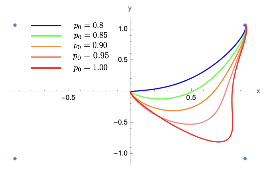
Where c±c_{\pm} is the central charge for the two CFTs on either side of the RG interface. The g-factor is given by the second and third term in (5.2). For a Janus interface we have c+=c−=cc_{+}=c_{-}=c, whereas the central charges differ on both sides of the interface for a RG-flow interface. It is straightforward to determine the R±R_{\pm} and ln⁡λ±\ln\lambda_{\pm} by numerically fitting the metric functions (see plot (c) in figures 4 and 5) to determine the slope and the intercept (5.5) in the limit of large |u||u|. We will give an example of numerical results by presenting the g-factors as for the RG-interface between the 𝒩=(4,4)\mathcal{N}=(4,4) vacuum and a 𝒩=(1,1)\mathcal{N}=(1,1) vacuum in truncation 2. As discussed in section 4.2 there exists a unique RG-flow interface for a choice on initial condition p0p_{0}. In figure 7 we present the g-factor as a function of the initial condition for a particular value of α=1.4\alpha=1.4.

Refer to caption
(a)
Refer to caption
(b)
Figure 7: (a) Plot of boundary entropy for RG-flow interface for truncation 2, as a function of initial condition p0p_{0} at the turning point for α=1.4\alpha=1.4. (b) Illustration of RG-flows for some initial values of p0p_{0}.

6 Discussion

In this paper we found holographic interface solutions in three dimensional gauged supergravity theories. An important feature of these theories is that they have AdS vacua which preserve 𝒩=(1,1)\mathcal{N}=(1,1) supersymmetry in addition to the 𝒩=(4,4)\mathcal{N}=(4,4) AdS vacuum. This feature allows us to find solutions which correspond to interfaces between two 𝒩=(4,4)\mathcal{N}=(4,4) vacua on both side, 𝒩=(1,1)\mathcal{N}=(1,1) on both sides, as well as RG-flow interfaces which have a 𝒩=(4,4)\mathcal{N}=(4,4) on one side and 𝒩=(1,1)\mathcal{N}=(1,1) vacuum on the other. We derived BPS flow equations which are three first order nonlinear differential equations for the two scalars p,qp,q which are non zero in the truncations as well as the warp factor BB of the A​d​S2AdS_{2} slicing. By using the freedom to shift the warping coordinate uu by a constant we can choose the initial conditions for the flow as the value of pp and qq at the turning point of the warp factor, where B′=0B^{\prime}=0. In fact we use the BPS equations to determine the initial conditions for the second order equation motion following from the variation of the action. The numerical accuracy of the solution is tested by checking the BPS equations away from the point where the initial conditions were fixed.

The 𝒩=(1,1)\mathcal{N}=(1,1) extrema are repulsive fixed points of the flow and hence the initial condition have to be fine tuned using a shooting method. This is possible by fixing one scalar initial condition and varying the other in order to come closer and closer to the 𝒩=(1,1)\mathcal{N}=(1,1) vacuum in the flow. Our results indicate that the qualitative behavior of the solutions for general α\alpha is quite similar to the behavior of the α=1\alpha=1 solutions obtained in [1]. In addition we have considered the entanglement entropy for the Janus and RG-flow solutions. Since for the RG-flow solutions the central charges and hence AdS radii are different on both sides of the interface one has to carefully consider the UV cut-off. It is possible to determine the g-function or interface entropy from the numerical solution by a linear fit of the warp factor BB.

We have considered truncations of the scalars to two nonzero scalars qq and pp (or xx and yy), it would be interesting to generalize this since it would then be possible to consider more complicated flows between different 𝒩=(1,1)\mathcal{N}=(1,1) vacua. It would also be interesting to investigate the solutions we have found can be lifted and have a representation in AdS3×S3×S3×S1\text{AdS}_{3}\times S^{3}\times S^{3}\times S^{1} holography. It would also be interesting to see whether the prescription for the interface entropy can be applied to other examples of RG-flow interfaces. We leave these interesting questions for future work.

Acknowledgements

The work of M. G. was supported, in part, by the National Science Foundation under grant PHY-19-14412. The authors are grateful to Kevin Chen for initial collaboration. The authors are grateful to the Mani L. Bhaumik Institute for Theoretical Physics for support.

Appendix A SO⁡(8)\SO(8) Gamma matrices

The formulation of the N=8N=8 three dimensional gauged supergravity utilizes with 8×88\times 8 Gamma matrices ΓA​A˙I\Gamma^{I}_{A\dot{A}} and their transposes ΓA˙​AI\Gamma^{I}_{\dot{A}A}, they satisfy the Clifford algebra,

ΓA​A˙I​ΓA˙​BJ+ΓA​A˙J​ΓA˙​BI=2​δI​J​δA​B\displaystyle\Gamma^{I}_{A\dot{A}}\Gamma^{J}_{\dot{A}B}+\Gamma^{J}_{A\dot{A}}\Gamma^{I}_{\dot{A}B}=2\delta^{IJ}\delta_{AB} (A.1)

Explicitly, we use the basis as given in Green-Schwarz-Witten [42],

ΓA​A˙8\displaystyle\Gamma^{8}_{A\dot{A}} =1⊗1⊗1,\displaystyle=1\otimes 1\otimes 1~, ΓA​A˙1\displaystyle\Gamma^{1}_{A\dot{A}} =i​σ2⊗i​σ2⊗i​σ2\displaystyle=i\sigma_{2}\otimes i\sigma_{2}\otimes i\sigma_{2}
ΓA​A˙2\displaystyle\Gamma^{2}_{A\dot{A}} =1⊗σ1⊗i​σ2,\displaystyle=1\otimes\sigma_{1}\otimes i\sigma_{2}~, ΓA​A˙3\displaystyle\Gamma^{3}_{A\dot{A}} =1⊗σ3⊗i​σ2\displaystyle=1\otimes\sigma_{3}\otimes i\sigma_{2}
ΓA​A˙4\displaystyle\Gamma^{4}_{A\dot{A}} =σ1⊗i​σ2⊗1,\displaystyle=\sigma_{1}\otimes i\sigma_{2}\otimes 1~, ΓA​A˙5\displaystyle\Gamma^{5}_{A\dot{A}} =σ3⊗i​σ2⊗1\displaystyle=\sigma_{3}\otimes i\sigma_{2}\otimes 1
ΓA​A˙6\displaystyle\Gamma^{6}_{A\dot{A}} =i​σ2⊗1⊗σ1,\displaystyle=i\sigma_{2}\otimes 1\otimes\sigma_{1}~, ΓA​A˙7\displaystyle\Gamma^{7}_{A\dot{A}} =i​σ2⊗1⊗σ3\displaystyle=i\sigma_{2}\otimes 1\otimes\sigma_{3} (A.2)

The matrices ΓA​BI​J\Gamma^{IJ}_{AB}, ΓA˙​B˙I​J\Gamma^{IJ}_{\dot{A}\dot{B}} and similar are defined as antisymmetrized products of Γ\Gammas with the appropriate indices contracted. For example,

ΓA​BI​J≡12​(ΓA​A˙I​ΓA˙​BJ−ΓA​A˙J​ΓA˙​BI)\displaystyle\Gamma^{IJ}_{AB}\equiv\frac{1}{2}(\Gamma^{I}_{A\dot{A}}\Gamma^{J}_{\dot{A}B}-\Gamma^{J}_{A\dot{A}}\Gamma^{I}_{\dot{A}B}) (A.3)

References

  • [1] K. Chen, M. Gutperle and C. Hultgreen-Mena, “Janus and RG-flow interfaces in three-dimensional gauged supergravity,” JHEP 03 (2022), 057 [arXiv:2111.01839 [hep-th]].
  • [2] D. Bak, M. Gutperle and S. Hirano, “A Dilatonic deformation of AdS(5) and its field theory dual,” JHEP 05 (2003), 072 [arXiv:hep-th/0304129 [hep-th]].
  • [3] A. B. Clark, D. Z. Freedman, A. Karch and M. Schnabl, “Dual of the Janus solution: An interface conformal field theory,” Phys. Rev. D 71 (2005), 066003 [arXiv:hep-th/0407073 [hep-th]].
  • [4] E. D’Hoker, J. Estes and M. Gutperle, “Exact half-BPS Type IIB interface solutions. I. Local solution and supersymmetric Janus,” JHEP 06 (2007), 021 [arXiv:0705.0022 [hep-th]].
  • [5] E. D’Hoker, J. Estes and M. Gutperle, “Interface Yang-Mills, supersymmetry, and Janus,” Nucl. Phys. B 753 (2006), 16-41 [arXiv:hep-th/0603013 [hep-th]].
  • [6] D. Gaiotto and E. Witten, “S-Duality of Boundary Conditions In N=4 Super Yang-Mills Theory,” Adv. Theor. Math. Phys. 13 (2009) no.3, 721-896 [arXiv:0807.3720 [hep-th]].
  • [7] D. Gaiotto and E. Witten, “Janus Configurations, Chern-Simons Couplings, And The theta-Angle in N=4 Super Yang-Mills Theory,” JHEP 06 (2010), 097 [arXiv:0804.2907 [hep-th]].
  • [8] E. D’Hoker, J. Estes and M. Gutperle, “Ten-dimensional supersymmetric Janus solutions,” Nucl. Phys. B 757 (2006), 79-116 [arXiv:hep-th/0603012 [hep-th]].
  • [9] E. D’Hoker, J. Estes, M. Gutperle and D. Krym, “Janus solutions in M-theory,” JHEP 06 (2009), 018 [arXiv:0904.3313 [hep-th]].
  • [10] E. D’Hoker, J. Estes and M. Gutperle, “Exact half-BPS Type IIB interface solutions. II. Flux solutions and multi-Janus,” JHEP 06 (2007), 022 [arXiv:0705.0024 [hep-th]].
  • [11] C. Bachas, E. D’Hoker, J. Estes and D. Krym, “M-theory Solutions Invariant under D⁡(2,1,γ)⊕D⁡(2,1,γ)D(2,1;\gamma)\oplus D(2,1;\gamma),” Fortsch. Phys. 62 (2014), 207-254 [arXiv:1312.5477 [hep-th]].
  • [12] K. Pilch, A. Tyukov and N. P. Warner, “𝒩=2\mathcal{N}=2 Supersymmetric Janus Solutions and Flows: From Gauged Supergravity to M Theory,” JHEP 05 (2016), 005 [arXiv:1510.08090 [hep-th]].
  • [13] M. Gutperle, J. Kaidi and H. Raj, “Janus solutions in six-dimensional gauged supergravity,” JHEP 12 (2017), 018 [arXiv:1709.09204 [hep-th]].
  • [14] M. Suh, “Supersymmetric Janus solutions in five and ten dimensions,” JHEP 09 (2011), 064 [arXiv:1107.2796 [hep-th]].
  • [15] N. Bobev, K. Pilch and N. P. Warner, “Supersymmetric Janus Solutions in Four Dimensions,” JHEP 06 (2014), 058 [arXiv:1311.4883 [hep-th]].
  • [16] A. Clark and A. Karch, “Super Janus,” JHEP 10 (2005), 094 [arXiv:hep-th/0506265 [hep-th]].
  • [17] M. Suh, “Supersymmetric Janus solutions of dyonic I​S​O​(7)ISO(7)-gauged 𝒩= 8\mathcal{N}\,=\,8 supergravity,” JHEP 04 (2018), 109 [arXiv:1803.00041 [hep-th]].
  • [18] P. Karndumri, “Supersymmetric Janus solutions in four-dimensional N=3 gauged supergravity,” Phys. Rev. D 93 (2016) no.12, 125012 [arXiv:1604.06007 [hep-th]].
  • [19] P. Karndumri and C. Maneerat, “Supersymmetric Janus solutions in ω\omega-deformed N=8N=8 gauged supergravity,” Eur. Phys. J. C 81 (2021) no.9, 801 [arXiv:2012.15763 [hep-th]].
  • [20] M. Chiodaroli, M. Gutperle and D. Krym, “Half-BPS Solutions locally asymptotic to AdS3xS∗3AdS_{3}xS*^{3} and interface conformal field theories,” JHEP 02 (2010), 066 [arXiv:0910.0466 [hep-th]].
  • [21] T. Assawasowan and P. Karndumri, “New supersymmetric Janus solutions from N=4 gauged supergravity,” Phys. Rev. D 105 (2022), 106004 [arXiv:2203.03413 [hep-th]].
  • [22] P. Karndumri and C. Maneerat, “Janus solutions from dyonic ISO(7) maximal gauged supergravity,” JHEP 10 (2021), 117 [arXiv:2108.13398 [hep-th]].
  • [23] D. Gaiotto, “Domain Walls for Two-Dimensional Renormalization Group Flows,” JHEP 12 (2012), 103 [arXiv:1201.0767 [hep-th]].
  • [24] M. Gutperle and J. Samani, “Holographic RG-flows and Boundary CFTs,” Phys. Rev. D 86 (2012), 106007 [arXiv:1207.7325 [hep-th]].
  • [25] I. Arav, K. C. M. Cheung, J. P. Gauntlett, M. M. Roberts and C. Rosen, “Superconformal RG interfaces in holography,” JHEP 11 (2020), 168 [arXiv:2007.07891 [hep-th]].
  • [26] Y. Korovin, “First order formalism for the holographic duals of defect CFTs,” JHEP 04 (2014), 152 [arXiv:1312.0089 [hep-th]].
  • [27] H. Nicolai and H. Samtleben, “N=8 matter coupled AdS(3) supergravities,” Phys. Lett. B 514 (2001), 165-172 [arXiv:hep-th/0106153 [hep-th]].
  • [28] M. Berg and H. Samtleben, “An Exact holographic RG flow between 2-d conformal fixed points,” JHEP 05 (2002), 006 [arXiv:hep-th/0112154 [hep-th]].
  • [29] H. J. Boonstra, B. Peeters and K. Skenderis, “Brane intersections, anti-de Sitter space-times and dual superconformal theories,” Nucl. Phys. B 533 (1998), 127-162 [arXiv:hep-th/9803231 [hep-th]].
  • [30] S. Elitzur, O. Feinerman, A. Giveon and D. Tsabar, “String theory on AdS(3) x S**3 x S**3 x S**1,” Phys. Lett. B 449 (1999), 180-186 [arXiv:hep-th/9811245 [hep-th]].
  • [31] J. de Boer, A. Pasquinucci and K. Skenderis, “AdS / CFT dualities involving large 2-D N=4 superconformal symmetry,” Adv. Theor. Math. Phys. 3 (1999), 577-614 [arXiv:hep-th/9904073 [hep-th]].
  • [32] S. Gukov, E. Martinec, G. W. Moore and A. Strominger, “The Search for a holographic dual to AdS(3) x S**3 x S**3 x S**1,” Adv. Theor. Math. Phys. 9 (2005), 435-525 [arXiv:hep-th/0403090 [hep-th]].
  • [33] B. de Wit, I. Herger and H. Samtleben, “Gauged locally supersymmetric D = 3 nonlinear sigma models,” Nucl. Phys. B 671 (2003), 175-216 [arXiv:hep-th/0307006 [hep-th]].
  • [34] T. Azeyanagi, A. Karch, T. Takayanagi and E. G. Thompson, “Holographic calculation of boundary entropy,” JHEP 03 (2008), 054 [arXiv:0712.1850 [hep-th]].
  • [35] M. Chiodaroli, M. Gutperle and L. Y. Hung, “Boundary entropy of supersymmetric Janus solutions,” JHEP 09 (2010), 082 [arXiv:1005.4433 [hep-th]].
  • [36] M. Gutperle and J. D. Miller, “Entanglement entropy at holographic interfaces,” Phys. Rev. D 93 (2016) no.2, 026006 [arXiv:1511.08955 [hep-th]].
  • [37] K. Jensen and A. O’Bannon, “Holography, Entanglement Entropy, and Conformal Field Theories with Boundaries or Defects,” Phys. Rev. D 88 (2013) no.10, 106006 [arXiv:1309.4523 [hep-th]].
  • [38] J. Estes, K. Jensen, A. O’Bannon, E. Tsatis and T. Wrase, “On Holographic Defect Entropy,” JHEP 05 (2014), 084 [arXiv:1403.6475 [hep-th]].
  • [39] I. Affleck and A. W. W. Ludwig, “Universal noninteger ’ground state degeneracy’ in critical quantum systems,” Phys. Rev. Lett. 67 (1991), 161-164
  • [40] M. Bianchi, D. Z. Freedman and K. Skenderis, “How to go with an RG flow,” JHEP 08 (2001), 041 [arXiv:hep-th/0105276 [hep-th]].
  • [41] S. Ryu and T. Takayanagi, “Holographic derivation of entanglement entropy from AdS/CFT,” Phys. Rev. Lett. 96 (2006), 181602 [arXiv:hep-th/0603001 [hep-th]].
  • [42] M. B. Green, J. H. Schwarz and E. Witten, “SUPERSTRING THEORY. VOL. 1: INTRODUCTION,” Cambridge, 1987