- 4G
- fourth generation
- 5G
- fifth generation
- AoA
- angle of arrival
- AoD
- angle of departure
- AP
- access point
- BCRLB
- Bayesian CRLB
- BS
- base stations
- BPP
- binomial point process
- BP
- broadcast probing
- CDF
- cumulative density function
- CF
- closed-form
- CRLB
- Cramer-Rao lower bound
- ECDF
- empirical cumulative distribution function
- EI
- Exponential Integral
- eMBB
- enhanced mobile broadband
- FIM
- Fisher Information Matrix
- GoF
- goodness-of-fit
- GPS
- global positioning system
- GE
- group exploration
- GNSS
- global navigation satellite system
- HetNets
- heterogeneous networks
- IoT
- internet of things
- IIoT
- industrial internet of things
- LOS
- line of sight
- MAB
- multi-armed bandit
- MBS
- macro base station
- MEC
- mobile-edge computing
- mIoT
- massive internet of things
- MIMO
- multiple input multiple output
- mm-wave
- millimeter wave
- mMTC
- massive machine-type communications
- MS
- mobile station
- MVUE
- minimum-variance unbiased estimator
- NLOS
- non line-of-sight
- OFDM
- orthogonal frequency division multiplexing
- probability density function
- PGF
- probability generating functional
- PLCP
- Poisson line Cox process
- PLT
- Poisson line tessellation
- PLP
- Poisson line process
- PPP
- Poisson point process
- PV
- Poisson-Voronoi
- QoS
- quality of service
- RAT
- radio access technique
- RL
- reinforcement-learning
- RSSI
- received signal-strength indicator
- BS
- base station
- SINR
- signal to interference plus noise ratio
- SNR
- signal to noise ratio
- SWIPT
- simultaneous wireless information and power transfer
- TS
- Thompson Sampling
- TS-CD
- TS with change-detection
- KS
- Kolmogorov-Smirnov
- UCB
- upper confidence bound
- ULA
- uniform linear array
- UE
- user equipment
- URLLC
- ultra-reliable low-latency communications
- V2V
- vehicle-to-vehicle
- wpt
- wireless power transfer
Fast Change Identification in Multi-Play Bandits and its Applications in Wireless Networks
Abstract
Next-generation wireless services are characterized by a diverse set of requirements, to sustain which, the wireless access points need to probe the users in the network periodically. In this regard, we study a novel multi-armed bandit (MAB) setting that mandates probing all the arms periodically while keeping track of the best current arm in a non-stationary environment. In particular, we develop TS-GE that balances the regret guarantees of classical Thompson sampling (TS) with the broadcast probing (BP) of all the arms simultaneously in order to actively detect a change in the reward distributions. The main innovation in the algorithm is in identifying the changed arm by an optional subroutine called group exploration (GE) that scales as for a armed bandit setting. We characterize the probability of missed detection and the probability of false-alarm in terms of the environment parameters. We highlight the conditions in which the regret guarantee of TS-GE outperforms that of the state-of-the-art algorithms, in particular, ADSWITCH and M-UCB. We demonstrate the efficacy of TS-GE by employing it in two wireless system application - task offloading in mobile-edge computing (MEC) and an industrial internet-of-things (IIoT) network designed for simultaneous wireless information and power transfer (SWIPT).
Index Terms:
Multi-armed bandits, Thompson sampling, Non-stationarity, Online learning.I Introduction
Sequential decision making problems in RL (RL) are popularly formulated using the MAB (MAB) framework, wherein, an agent (or player) selects one or multiple options (called arms) out of a set of arms at each time slot [1, 2, 3, 4, 5]. Each time the player selects an arm or a group of arms, it receives a reward characterized by the reward distribution of the played arm/arms. The player performs consecutive action-selections based on its current estimate of the reward (or that of its distribution) of the arms. The player updates its belief of the played arms based on the reward received. In case the reward distribution of the arms is stationary, several algorithms have been shown to perform optimally [6]. On the contrary, most real-world applications such as IoT (IoT) networks [7], wireless communications [8], computational advertisement [9], and portfolio optimization [10] are better characterized by non-stationary rewards. However, non-stationarity in reward distributions are notoriously difficult to handle analytically.
To address non-stationarity, researchers either i) construct passively-adaptive algorithms that are change-point agnostic and work by discounting the impact of past rewards gradually or ii) derive frameworks to actively detect the changes in the environment. Among the actively-adaptive algorithms, the state-of-the-art solutions, e.g., ADSWITCH by Auer et al. [11] provide a regret guarantee of for a -armed bandit setting experiencing changes in a time-horizon . Recently, researchers have also explored predictive sampling frameworks for tackling non-stationarity [12]. There the authors developed an algorithm that deprioritizes investment in acquiring information that will quickly lose relevance.
Contrary to most non-stationary bandit algorithms, in several applications, the agent can possibly select multiple arms simultaneously. In such cases, the agent may either have access to the individual rewards of the arms played or a function of the rewards. For example, authors in [13] explored a wireless communication setup where a user can select multiple channels to sense and access simultaneously. Similarly, in portfolio optimization [14] multiple plays refers to investing in multiple financial instruments simultaneously. However, to the best of our knowledge, none of the existing works investigate multiple simultaneous plays under a changing environment.
In contrast to this we propose an algorithm based on grouped probing of the arms that identifies the arm that has undergone a change in its mean. We investigate the conditions under which the proposed algorithm achieves superior regret guarantees than the state-of-the-art algorithms.
I-A Related Work
Non-stationarity Actively-adaptive algorithms have been experimentally shown to perform better than the passively-adaptive ones [15]. In particular, ADAPT-EVE, detects abrupt changes via the Page-Hinkley statistical test (PHT) [16]. However, their evaluation is empirical without any regret guarantees. Similarly, another work [10] employs the Kolmogorov-Smirnov statistical test to detect a change in distribution of the arms. Interestingly, tests such as the PHT has been applied in different contexts in bandit frameworks, e.g., to adapt the window length of SW-UCL [17]. The results by [18, 19], and by Cao et al. [20] detect a change in the empirical means of the rewards of the arms by assuming a constant number of changes within an interval. While the algorithm in [20], called M-UCB achieves a regret bound of , the work by Yu et al. leverages side-information to achieve a regret of . However, the proposed algorithms in both these works assume a prior knowledge of either the number of changes or the change frequency. On these lines, recently, Auer et al. [11] have proposed ADSWITCH based on the mean-estimation based checks for all the arms. Remarkably, the authors show regret guarantees of the order of for ADSWITCH without any pre-condition on the number of changes for the -arm bandit problem. If the number of changes is known, a safeguard against a change in an inferior arm can be achieved by sampling it in inverse proportion of its sub-optimality gap . This achieves a regret of . However, if the number of changes is not known, setting the sampling rate is challenging and if the number of changes is greater than , several algorithms experience linear regret. In order to avoid this, the main idea in ADSWITCH is to draw consecutive samples from arms, thereby incurring a regret that scales as in the worst-case. Nevertheless, since both M-UCB and ADSWITCH provide the same regret guarantees, we choose them as the competitor algorithms for our proposal.
Multiple Plays: The paper by Anantharam et al. [21] is one of the first works that introduced the concept of multiple plays. Apart from the work by [13], others that have investigated bandits with multiple plays include [22] which considered budgeted settings for multiple plays with random rewards and cost. In the context of distributed channel access, [23] explored the setting where multiple agents accessing the same arm simultaneously. Its important to note that a multi-player setting is different than a single-player multi-play setting as considered in this paper. Multi-player bandits may lead to collisions which can be resolved in several ways, e.g., equal division of reward. We refer the reader to the work by Besson et al. [24] for a discussion on this. For multi-play bandits that include multiple players, the recent work by Wang et al. [25] consider a per-load reward distribution and prove a sample complexity lower bound for Gaussian distribution. Nevertheless, none of these existing works treat multiple plays under non-stationarity which can dramatically alter the policy of the player. In particular, a missed-detection due to the change occurring in a less sampled arm can lead to a worst-case linear regret.
Frequency of Probing: Zhou et al. [26] have studied a framework for joint status sampling and updating in IoT networks. The authors formulated the problem as an infinite horizon average cost constrained Markov decision process. The policy for a single IoT device is derived and a trade-off is revealed between the average age of information and the sampling and updating costs. The work by Stahlbuhk et al. [27] considers a system consisting of a single transceiver pair and a set of communication channels to chose from. They devise a policy to minimize the queue length regret, for which they provide a regret guarantee of the order of . A rigorous analysis for the regret of age-of-information bandits was presented in [28], where first it is shown that UCB and Thompson sampling are order-optimal for AoI bandits. Then a novel algorithm is proposed that performs the classical algorithms by making AoI aware decisions. However to the best of our knowledge, none of these works consider the environment to be non-stationary which limits their applicability in modern wireless systems.
I-B Motivation and Contribution
Unlike M-UCB but similar to ADSWITCH, we consider a framework where the number of changes is not known a-priori but to be fewer than . Furthermore, we target an additional requirement - the agent algorithm should guarantee that the age between two consecutive plays of each arm is bounded. Although the issue of age has previously been addressed in some works (e.g., see [28]), the solutions cater to stationary environments. On the contrary, in this work, under an assumption of the hard-core distance between two consecutive changes, we propose TS-GE which outperforms ADSWITCH and M-UCB under several regimes of and the time-horizon, , while simultaneously satisfying the mandatory probing requirement. The major innovation in this paper is two-fold - i) by allowing simultaneous probing of multiple arms in a coded manner, we reduce the scaling of changed-arm identification form to , and ii) by design, TS-GE guarantees that the last sample of each arm is not older than . Overall, the main contributions of this paper are:
- •
We develop and characterize TS-GE, tuned for non-stationary environments with unknown number of change-points. The additional design guarantee of TS-GE is the periodic mandatory probing of all the arms. Although this is relevant for several applications, to the best of our knowledge, this requirement has not been treated previously in literature. By balancing the regret guarantees of stationary Thompson sampling with grouped probing of all the arms, TS-GE ensures an upper bound of in the sampling age of each arm.
- •
We propose a coded grouping of the arms based on the arm indices and consequently, derive the probability of missed detection of change and the probability of false alarm and highlight the conditions to limit these probabilities. Based on this, we show that TS-GE achieves sub-linear regret, . We compare this bound with the best known bound of and discuss the conditions under which the bound of TS-GE outperforms the latter. A summary of the pros and cons of our proposal is presented in Table I.
- •
As the first case-study, we employ TS-GE as a strategy for wireless nodes to offload their computational tasks to a set of MEC (MEC) servers. We demonstrate how the grouped probing phase of the algorithm enables the users to keep track of the best server to offload their tasks under a dynamic environment.
- •
Finally, as the second case-study, we consider an IIoT (IIoT) network where a central controller is required to sustain SWIPT (SWIPT) services to the IoT devices. The different phases of TS-GE are mapped to the data-transfer and energy-transfer operations of the network. We demonstrate the performance of TS-GE with respect to the statistical upper-bound derived using stochastic geometry tools. Contrary to our proposal, in other algorithms such as M-UCB the exists non-zero probability that the IoT devices do not receive any energy transfer and hence our proposal will find applications that constrain sample age.
The rest of the paper is organized as follows. In Section II we describe the system model and the problem setup. The proposed algorithm TS-GE algorithm is presented in Section III. The mathematical analysis of missed detection, false alarm, and the regret analysis is presented in Section IV. Then, Section V discusses the salient features of the derived regret bound. In order to test the efficacy of the proposed framework, we employ TS-GE in two case studies in Section VI-A and Section VI-B. Finally, the paper concludes in Section VII. The notations used in the paper are summarized in Table II
| Feature | This paper | Benchmark [20, 11] |
|---|---|---|
| Scaling with | (after initialization) | |
| Guarantee on change-detection latency | No guarantee | |
| Scaling with | Worst case - | |
| Scaling with | ||
| Additional requirement | Multiple-simultaneous plays | - |
| Symbol | Definition |
|---|---|
| , | Set of arms, number of arms. |
| , , | th arm, its mean at time , estimate of the mean at |
| Time horizon | |
| Number of changes | |
| Arm pulled at time | |
| Reward of arm at time | |
| Reward obtained by policy at time | |
| Success/Failure event observed by policy at time | |
| Probability that an episode experiences a change | |
| Probability that one slot experiences a change | |
| Regret experienced by a policy at time | |
| Length of each episode | |
| Length of each TS (TS) phase | |
| Length of each BP (BP) phase | |
| Length of each GE (GE) phase | |
| TS parameters of arm | |
| th super arm |
II Problem Setup

Consider a -arm bandit setting with arms , where . For the discussion in this paper, let us assume that for some . It may be noted that in case the number of arms is not a power of 2, the same can be transformed into one by adding dummy arms which are sub-optimal with a probability 1 (e.g., arms with a constant reward of ). The policy of the player is denoted by . In other words refers to the player pulling arm at time .
Reward distribution: The reward of an arm at time is assumed to be an instance of a truncated Gaussian random variable with mean , variance , and truncation limits and [29]. This assumption is valid for most practical wireless applications, e.g., upper bound on received power, SINR (SINR), or data-rate by the wireless nodes. We note that the regret guarantees derived in this paper holds for any sub-Gaussian distribition of the rewards. The assumption of the trunctated Gaussian is
It is worth to note that according to the above, the variance of all the arms is constant and is the same for all arms11 1 This assumption is simply due to the ease of notations and the derivation of the regret bounds. The algorithm can be executed with this assumption does not hold. However, the regret analysis for such a case is much more involved and will be investigated in a future work., however, the mean is a function of time.
Success/Failure events: Furthermore, we assume that in addition to the reward, the player observes a success or failure event corresponding to each given that . The value of is drawn from a Bernoulli distribution with parameter . For example, in latency-constrained networks, may correspond to the transmission SINR, while corresponds to the event of successful packet reception which depends not only on but also on other network parameters such as cell-load. It is precisely this uncertainty that we model using the Bernoulli trial. We note that the agent has access to both and . The availability of the with the player naturally leads to the choice of Beta priors in the TS phase of our algorithm.
Multiple plays: Finally, we assume that at any time-slot, multiple arms can be played by the agent. However, in that case, the agent observes a weighted average of the rewards of the pulled arms. This is formally mentioned below.
Assumption 1.
In case at any time-slot the policy pulls multiple (say ) arms, i.e., , then the reward observed by the player is
Note that the player does not have access to the individual arm rewards of the set of arms it has played. This model fits into several application setting, for example, when the bandwidth is divided among users equally, the network throughput is times the sum of spectral efficiency experienced by each user. At this stage, we note that such an assumption is not present in [11] as highlighted in Table I.
II-A Non-stationarity model
Mandatory probing requirement: The player interacts with the bandit framework in a sequence of episodes, denoted by , , each of length . Consequently, the total time-horizon can be expressed as . It is important to note that the episodes are a feature of the problem setting and the framework rather than that of the algorithm. The episodes impose a condition on any feasible policy of the player as stated below.
Condition 1.
The framework mandates that each arm be probed (either individually or in a group) at least once in each episode.
This condition corresponds to applications such as mandatory status-updates or timely wireless power transfer in IoT networks.
Change model: We assume a piece-wise stationary environment in which changes in the reward distribution occur at time slots called change points, denoted by , , where each . At each change point, exactly one of the arms , uniformly selected from experiences a change (increase or decrease) in its mean by an unknown amount . Furthermore, we assume that during each episode, at most one change point occurs with a probability and the total number of changes is within , which is unknown to the player. In particular, at in each episode, at the beginning of each time slot, the environment samples a Bernoulli random variable with success probability . In case of a success, the change occurs in that slot, while in case of a failure, the bandit framework does not change. Once a change occurs in an episode, the change framework is paused until the next episode. Thus,
where, . As a practical analogy, this change framework can be related to the state of a MEC server admitting new tasks at each episode. Let an edge device attempt to offload its task to the MEC server at each time slot. The event of successful admission of the task depends on the server state, the channel conditions, the computational requirement, etc. On an offload failure, let the edge device attempt an offload again in the next slot wherein the server state and the computational requirement is assumed to remain same, while the channel state can be considered to be and identical and independent realization of the previous slot. The probability of a successful offload can be assumed to be . Once such a new task is admitted in the server, its state changes and it freezes further admitting new tasks until the rest of the episode. This will be discussed in detail in Section VI-B.
II-B Policy Design
The challenge for the player is to quickly identify changes that any arm has undergone and adapt its corresponding parameters. For benchmarking the performance of a candidate player policy, at a given time slot, a policy competes against a policy class which selects the arm with the maximum expected reward at that time slot. Thus, any policy that intends to balance between the exploration-exploitation trade-off of the bandit framework experiences a regret
| (1) |
where is the mean of the arm picked by the policy at time . It can be noted here that unlike stationary environments, the identity of the best arm , where, is not fixed and may change with at each change point.
III TS-GE: Algorithm Description and Features
The key features of our proposed algorithm TS-GE are i) actively detecting the change in the bandit framework, ii) identifying the arm which has undergone a change, and iii) modify its probability of getting selected in the further rounds based on the amount of change. The TS-GE algorithm consists of an initialization phase called explore-then-commit, ETC, followed by two alternating phases: classical TS phase followed by a BP phase to determine a change in the system. In case a change is detected in the BP phase, the arm which has undergone a change is identified using an optional sub-routine called GE. Thus, the GE phase is only triggered if a change is detected in the BP phase. The overall algorithm is illustrated in Fig. 1 and presented in Algorithm 1. Each consists of one TS phase, one BP phase, and (optionally) one GE phase.
III-A Initialization: ETC for TS-GE
For initialization, the player performs a ETC for TS-GE, wherein each arm is played an number of times and consequently, their mean is estimated to be .
Definition 1.
An arm is defined to be well-localized if the empirical estimate of its mean is bounded as
III-B Alternating TS and BP phases
Each episode consists of a TS phase, a BP phase, and an optional GE phase. Since in practical scenarios of interest, the time-horizon can be made arbitrary, let us set . In the TS phase, the player performs the action selection of the choices according to the TS algorithm for slots as given in [30]. The version of Agrawal and Goyal [30] can be implemented here due to the fact that the player has access to the binary rewards . Each arm is characterized by its TS parameters and , all of which are initially set to one22 2 Note that the TS parameters can be initialized according to the observed rewards in the ETC phase. However, in order to safeguard against changes in the ETC phase, we begin the TS phase with fresh parameters.. After each play of an arm , its estimated mean is updated according to the reward from the truncated Gaussian distribution . Let be played at time slots and the number of times it is played is until (and including) the time-slot , then:
| (2) |
Additionally, the TS parameters for the played arm , i.e., and are updated as per a Bernoulli trial with a success probability each time is played.
Each TS phase is followed by the BP phase for time-slots, where the player samples all the arms simultaneously for rounds. During this phase, the reward observed by the player is the average of the rewards from all the arms, i.e., , for all the time slots in the BP phase. The reward in the BP phase is then compared with the average of the estimates of all the arms to detect whether an arm of the framework has changed its mean. Recall that as per Assumption 1, during the BP phase of the -th episode, the player receives the following reward for each play:
where represents the truncated Gaussian distribution with mean and variance . At the end of the -th BP phase, a change is detected if:
| (3) |
Here the first term is the average of the estimated means of all the arms at the end of the -th TS phase, while the second term represents the same evaluated during the -th BP phase. In case the change does not occur or goes undetected, the algorithm continues with the next TS phase. However, in case a change is detected or a false-alarm is generated, the algorithm moves on to the GE sub-routine as described below.
III-C Policy after change detection
If a change is detected in the BP phase, the GE phase begins for the identification of the changed arm. The key step in this phase is the creation of sets , called super arms as shown in Algorithm 2. Recall that is a number such that . It may be noted that an optimal grouping of arms may be derived that considers the fact that the arms that have been played a fewer number of times have a larger error variance of its mean estimate. However, such a study is out of scope for the current text and will be treated in a future work.
Arm Grouping Strategy: The -th arm, is added to a super arm , if and only if the binary representation of has a ”1” in the -th binary place. In other words, is added to if:
where and are respectively operators that convert binary numbers to decimals and decimal numbers to binary. Additionally, is a binary number with all zeros except 1 at the -th binary position. AND is the bit-wise AND operator. This strategy for creating super-arms is inspired from the classical forward error correcting strategy due to Hamming, which enables detection and correction of single-bit errors [31]. In the GE phase, each super arm is played times and the player obtains a reward which is the average of rewards of all the arms that belong to as per Assumption 1, i.e., each time the super arm is played, the player gets a reward that is sampled from the distribution:
Let the mean reward of the super arm be denoted by . Before the beginning of each GE phase, is estimated. As an example, let a change be detected after the -th BP phase. Then, the estimate of the mean reward of the super arm is:
| (4) |
Then, the arm with the changed mean is the one that belongs to the all super arms in which a change of mean is detected. For each super arm , the changed arm either is present in or it is present in its complimentary set . Let us define a new sequence of sets as
| (5) |
Then, the changed arm is identified as , where . In case no change is detected in any of the super arms, but the BP phase detects a change, the changed arm is identified as .

III-D Illustrative Example
Let us elaborate this further with the example of an illustrative example with . Fig. 2 shows the following grouping for the super arms -
- •
- Arms with ’1’ in the first decimal place - and .
- •
- Arms with ’1’ in the second decimal place - and .
- •
- Arms with ’1’ in the third decimal place - and .
- •
- Arms with ’1’ in the fourth decimal place - and .
Now, in case a change occurs in an arm, say arm , this will be detected in super arms and but not in and . Additionally, this combination of changes in the super arms uniquely corresponds to the arm . Similarly, a change only in the super arm and in no other super arms corresponds to a change in arm . Finally, note that no changes in any of the super arms (but a change detected in the BP phase) corresponds to a change in .
Once the change is detected and the changed arm is identified, the corresponding mean of is updated as
| (6) |
Furthermore, the TS parameters of the arm is updated. In particular, we set the parameters of to be same as the arm that has an estimated mean closest ot as:
In the next section we characterize the probability with which TS-GE misses detection a change or raises a false alarm in case of no change. This eventually leads to the regret.
| where |
IV Analysis of TS-GE
In this section we derive some conditional mathematical results for TS-GE. In particular, under conditions on the magnitude of change and a lower bound on the probability of change in each slot, we derive a sub-linear regret for TS-GE. First, let us note the following for the ETC phase.
Lemma 1.
In the stationary regime, in order for the arm to be well-localized with a probability , the arm needs to have been played at least times, where
Proof.
The proof follows from Hoeffding’s inequality for bounded random variables between 0 and . ∎
Thus, the ETC phase lasts for at least rounds. Naturally, in order to restrict to , needs to be . Then let us recall that the GE phase is triggered only if a change is detected in the BP phase. Consequently, the algorithm can miss detecting the chase in case the change occurs either in the TS phase or the BP phase, which we analyze below.
IV-A Probability of Missed Detection
Since the only condition on is that it has to be upper bounded by , let us set . Let the change occur in the arm at time slots in the -th TS phase, i.e., . The mean is assumed to change from to . In other words, the distribution of the reward of is given as:
The following lemma characterizes the probability of missed detection when the change occurs in the TS phase.
Lemma 2.
Let the arm change its mean from to , where at a time slot in the -th TS phase. Then, if , the probability of missed detection after the -th BP phase following this change is upper bounded by
Proof.
Please see Appendix A. ∎
Note that detecting relatively small changes is not only challenging but also becomes unnecessary in several practical applications. Accordingly, we assume a minimum quantum of change once such a change event occurs. The above result bounds the probability of missed detection in the TS phase to inversely proportional to T. However, if the change occurs in the BP phase, the probability of missed detection increases as discussed below.
Lemma 3.
Let the arm change its mean from to , where at a time slot in the -th BP phase. Furthermore, let be lower-bounded as
| (7) |
Then the probability of missed detection after the -th BP phase following this change has the following characteristic:
| (8) |
where, and .
Proof.
Please see Appendix B. ∎
First, let us note that since the right hand side of (7) is a decreasing function, for large values of , it is a fairly mild assumption. This lemma shows that a change in the BP phase results in a different probability of missed detection based on the exact point of change. In particular, from the proof we note that for cases 2 and 4, the algorithm misses the detection of the change in the BP phase with a high probability. However, these cases themselves occur with low probability due to the condition (7), which enables us to bound the probability of missed detection.
IV-B Probability of False Alarm
Another aspect of the algorithm that needs to be considered for a regret analysis is the fact that the BP phase can raise a false alarm when a change has not occurred in an episode while, the condition (3) holds true simultaneously. However, in case of no change, the test statistic is simply , where . Here is the number of times the arm has been played in all the TS phases. Thus,
| (9) |
IV-C On the Regret of TS-GE
Now we have all the necessary results to derive the following regret bound for TS-GE.
Theorem 1.
The regret for TS-GE under assumption and 7 is upper bounded as
| (10) |
Proof:
Please see Appendix C ∎Thus, not only the regret of TS-GE is sub-linear but also as discussed in the next section, it outperforms the known bounds under several regimes. Additionally, let us note that in most wireless system applications, the initialization phase occurs only once throughout a service session, e.g., initial access for wireless nodes or initial server allocation for edge devices. Hence, from a practical standpoint, the first term of the regret which scales linearly with does not impact long-term deployment of the algorithm.
V Discussion on Regret


.
In this section, we discuss the derived regret bound of TS-GE with respect to the best known bound of ADSWITCH [11] and M-UCB [20], Let us define three time slots , . and as follows:
- •
.
- •
, .
In other words, and are the time instants where the regret bound of TS-GE matches the bound of ADSWITCH or M-UCB. We compare the regret bounds for three different number of arms relevant for a massive IoT setup: small - arms, medium - arms, and large - arms. We consider a time-horizon of number of plays.
For , Fig. 3b shows that there are specific regions where TS-GE outperforms M-UCB. Beyond , M-UCB outperforms TS-GE. The point of interest for our discussion is the exact location of for different values of . For , the value of is low (see Fig. 3a) and the regret bound of M-UCB is lower than TS-GE for most part of the time-horizon. However, in case of , the value of is beyond the time-horizon, and accordingly, beyond time step 5000, throughout the time frame of interest, TS-GE outperforms M-UCB. This highlights the fact that the time-period of interest in a specific application would dictate the choice of a particular algorithm.
VI Case Studies in Wireless Networks
VI-A Case Study 1: Task Offloading in Edge-Computing
Let us consider a MEC cluster consisting of multiple edge servers33 3 The framework can also be implemented in dense cognitive radio networks with appropriate wireless propagation models.. The set of servers in the cluster is denoted by . The MEC cluster caters to two different classes of users - primary users and secondary users. The primary users are priority users that are guaranteed QoS (QoS) on admission. The association and admission of the primary users with the MEC servers are controlled centrally so as to provide performance guarantees to all the primary users. On the contrary, the secondary users opportunistically offload their tasks to selected servers based on their availability of compute resources. Unlike for the primary users, the secondary user requests can either be admitted or dropped depending on the current task load of the servers. Due to the dynamic traffic and mobility of the users, we consider that the primary user load on the servers changes with time. This dynamically alters the ability of the servers to admit new secondary user tasks. The availability of the servers is related by the workload buffer which characterizes the pending task load at a server as discussed next.
VI-A1 Temporal evolution of the workload buffer
The central controller updates the primary user and server connectivity periodically in epochs. At the beginning of each epoch, the central controller updates the status of at most one server. In particular, for the selected server , the controller admits new primary users with fresh requests and disconnects with the primary users that have already been served by the server. The selection of the server under consideration at each epoch follows the current server load, temporally dynamic traffic density, and channel conditions. In a given epoch, the controller may also decide to not update any server. The server selection policy for updates is unknown to the secondary users. Once the update period is over, it is followed by the service period for the primary and the secondary users simultaneously. The service period consists of multiple time-slots which lasts until the beginning of the next epoch. While each primary user is allotted a dedicated server with service guarantee, on the contrary, each secondary user chooses one or multiple servers during the service period to offload their computational task. In case multiple servers are selected by the secondary user, it partitions the task into segments of sub-tasks and sends to each corresponding server. Let the beginning of the th epoch be denoted by where . For an epoch , we denote the workload buffer size for server as . An admission control mechanism is assumed wherein a server accommodates a maximum workload buffer of . Let denote the number of admitted users in the server in epoch . The offload rate for the primary users and the total service rate for the server is assumed to be cycles/second and cycles/second, respectively. In case the th server changes its state in the th epoch, the size of the workload buffers evolves during as
| (11) |
VI-A2 Strategy for the secondary users
We model the task offloading process of a secondary-user in this network as the MAB problem. Recall that the secondary users are not aware of the state changes in the servers. However, they have information about the epochs. We map the TS-GE framework developed in this paper to the strategy of a single secondary user44 4 Consideration of collision among the requests of multiple secondary users at a single server is beyond the scope of this paper and will be treated in a future work.. In particular, the service period is mapped to the TS phase of the algorithm. Then, the update and association period of the next epoch corresponds to the BP and GE of an episode.
Let a secondary user attempts to offload a task which takes cycles to process. Based on the workload buffer, the time required by server to generate the output is calculated as:
| (12) |
We consider that the offloading is successful if the process output is generated within a compute deadline of the secondary user. Thus, the reward for selecting an arm in the TS phase is modeled as for Algorithm 1. In the BP phase, the edge user partitions its compute task into equal sub-tasks and attempts to offload a sub-task in each edge server. Naturally, the reward obtained by the user in such a case is the sum of the rewards for each sub-task. This naturally blends into the TS-GE algorithm for change detection and server identification.
VI-A3 Numerical Example
We employ the TS-GE framework in a MEC cluster with 128 servers. The maximum workload buffer is taken as 1 Giga-cycles, while in a given realization for a server the service rate is uniformly sampled from GHz. The value of is taken to be 8 Mbps and the task deadline is taken as 0.05 seconds. In order to highlight the change detection framework, we consider fixed change points across different realizations of the algorithms. Specifically, changes occur at episodes .
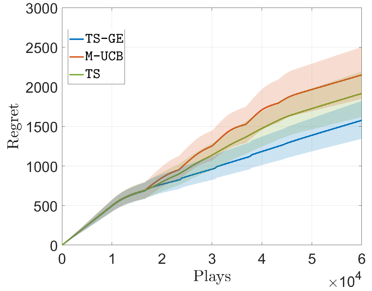
In Fig. 4, we compare the classical TS algorithm with TS-GE and M-UCB. We see that TS-GE outperforms the others by detecting the exact arm that has undergone a change. Interestingly, M-UCB performs worse than TS, mainly due to the fact that M-UCB flushes all the past (potentially relevant) rewards and restarts the exploration procedure once a system-level change is detected.
VI-B Case Study 2: SWIPT in an IIoT Network
In this section, we employ the TS-GE algorithm to evaluate an IIoT network where a central controller transmits data-packets to the device with the best channel condition and simultaneously performs wireless power transfer to all the devices.
VI-B1 Network Model
Let us consider an IIoT network consisting of a central wireless AP (AP) and IoT devices. The set of the devices is denoted by . Typically an industrial environment deals with a large that represent multiple sensors and cyber-physical systems. The AP provisions two wireless services in the network: i) periodic wpt (wpt) to all the IoT devices and ii) a unicast broadband data transmission to one selected IoT device55 5 The unicast service is relevant in cases when the AP intends to select the best storage-enabled IoT device to transfer large files for caching at the edge. This may then be accessed by the other IoT devices, e.g., using device-to-device link. However, in this paper, we do not delve deeper into such an analysis..
Let the scenario of interest be modeled as a two-dimensional disk of radius centered around the origin similar to [32]. The transmit power of the AP is . The location of the devices is assumed to be uniform in . Each AP-device link may be blocked by roaming blockages in the environment. The probability that a link of length is in LOS (LOS) is assumed to be [33]. Furthermore, note that due to the presence of a large number of metallic objects, an industrial scenario presents a dense scattering environment. Consequently, we assume that each transmission link experiences a fast-fading modeled as a Rayleigh distributed random variable with variance 1. Thus, The received power at an IoT device at a distance of from the AP is given by with a probability . Here and respectively are the path-loss coefficient and the path-loss exponent. The total transmission bandwidth is assumed to be which is orthogonally allotted to the users scheduled in one time-slot.
At each episode, the controller selects the device with the best channel conditions and executes information transfer in a sequence of time-slots using the TS phase of the algorithm. The device-specific transmission can be facilitated by employing techniques such as beamforming. However we do not consider the details of such procedures. The TS phase information transfer is followed by joint power transfer to all the devices. This is mapped to the BP phase of the algorithm. At the end of the BP phase, the total energy harvested at all the devices at the end of the BP phase is reported back to the controller. Using this total energy transfer report, the controller detects whether a change in the large-scale channel conditions has taken place. If so, then the controller probes multiple devices grouped together as per TS-GE to detect the device with the current best channel conditions.
VI-B2 Performance Bounds using Stochastic Geometry
Before proceeding with the evaluation of TS-GE in this network, let us first derive the upper bound on the statistical performance of data-rate. This will enable a comparison with not only an existing algorithm but also the performance limit. Since the location of the devices is assumed to be uniform across the factory floor, they form a realization of a BPP (BPP). Additionally, due to the assumption that the blockage in each link is independent of each other, the IoT devices are either in LOS or NLOS state. The probability that at least one of the IoT devices is in LOS state is given by:
The above expression follows similarly to [34]. On the same lines, the probability that at least one of the IoT devices is in NLOS state is given by
VI-B3 Best-link transmission for information transfer
Out of the possible IoT devices, the central controller selects the device with the best channel condition for information transfer. For that first, let us derive the distance distributions of the nearest LOS and NLOS devices.
Lemma 4.
The distribution of the distance to the nearest LOS device, and the nearest NLOS device, are respectively:
where,
Proof.
Using the void probabilities (see [35]) we have:
Evaluating the above series derives the result. The case for the NLOS device also follows in a similar manner. ∎
Across different realizations of the network, the best link experiences a fading-averaged downlink received power
| (14) |
Over a time-horizon of slots the throughput experienced by the system is
| (15) |
where the expectation taken over as per (14).
VI-B4 Multicast/Broadcast transmission for power transfer
Let us assume that in the multicast transmission phase, the AP transmits data to a subset of the IoT devices, where . In this case, the available bandwidth is shared among the devices. The harvested power experienced by an IoT device of is:
| (16) |
Accordingly, the network sum-energy is given by: in one slot. In case of the BP phase, naturally we have .
VI-B5 Numerical Example
We run the TS-GE algorithm in our IIoT network for a total of 1000 seconds with time-slots of 10 ms [36]. Additionally we assume slow moving blockages in which each 30 seconds the visibility state of exactly one IoT device changes from LOS to NLOS or vice-versa.

In Fig. 5 we plot the average throughput of the information transfer phase (i.e., to the best device) as well as the minimum harvested energy in a device in the IIoT network. We observe that in case of a fewer IoT devices, the M-UCB algorithm performs better than TS-GE. Indeed resetting all arms does not incur a large exploration loss in M-UCB in case is small. Additionally, M-UCB is not constrained by mandatory exploration. Accordingly, it enjoys a higher throughput as compared to TS-GE which needs to transfer energy all the devices.
Interestingly, as the number of devices in the network increases beyond a threshold, TS-GE outperforms M-UCB especially due to rapid changed state identification in the device. Naturally, as increases, the amount of time dedicated for energy transfer decreases. This is reflected in the reduced energy harvested in the worst device.
Several open problems are apparent. For example, the condition on that each episode can experience only one change can be too stringent to be applied meaningfully in contexts. Furthermore, change detection in the distributions rather than mean and extension to multiple players are indeed interesting directions of research which will be treated in a future work.
VII Conclusion
Existing multi-armed bandit algorithms that are tuned for non-stationary environments sample sub-optimal arms in a probabilistic manner in proportion to their sub-optimality gap. However, several applications require periodic mandatory probing of all the arms. To address this, we develop a novel algorithm called TS-GE which balances the regret guarantees of classical Thompson sampling with a periodic group-exploration phase which not only ensures the mandatory probing of all the arms but also acts as a mechanism to detect changes in the framework. We propose an index-based grouped probing strategy for fast identification of the changed arm. We show that the regret guarantees provided by TS-GE outperforms the state-of-the-art algorithms like M-UCB and ADSWITCH for several time-horizons, especially for a high number of arms. We demonstrated the efficacy of TS-GE in two wireless communication applications - edge offloading and an industrial IoT network designed for simultaneous wireless information and power transfer.
References
- [1] C. Shi and C. Shen, “Multi-player multi-armed bandits with collision-dependent reward distributions,” IEEE Transactions on Signal Processing, vol. 69, pp. 4385–4402, 2021.
- [2] C. Gan, R. Zhou, J. Yang, and C. Shen, “Cost-aware cascading bandits,” IEEE Transactions on Signal Processing, vol. 68, pp. 3692–3706, 2020.
- [3] A. Slivkins et al., “Introduction to multi-armed bandits,” Foundations and Trends® in Machine Learning, vol. 12, no. 1-2, pp. 1–286, 2019.
- [4] W. R. Thompson, “On the likelihood that one unknown probability exceeds another in view of the evidence of two samples,” Biometrika, vol. 25, no. 3/4, pp. 285–294, 1933.
- [5] J. Gittins, K. Glazebrook, and R. Weber, Multi-armed bandit allocation indices. John Wiley & Sons, 2011.
- [6] E. Contal, D. Buffoni, A. Robicquet, and N. Vayatis, “Parallel Gaussian process optimization with upper confidence bound and pure exploration,” in Joint European Conference on Machine Learning and Knowledge Discovery in Databases, pp. 225–240, Springer, 2013.
- [7] A. Uprety and D. B. Rawat, “Reinforcement learning for iot security: A comprehensive survey,” IEEE Internet of Things Journal, vol. 8, no. 11, pp. 8693–8706, 2020.
- [8] S. K. Singh, V. S. Borkar, and G. Kasbekar, “User association in dense mmwave networks as restless bandits,” IEEE Transactions on Vehicular Technology, pp. 1–1, 2022.
- [9] J. Huh and E. C. Malthouse, “Advancing computational advertising: Conceptualization of the field and future directions,” Journal of Advertising, vol. 49, no. 4, pp. 367–376, 2020.
- [10] G. Ghatak, H. Mohanty, and A. U. Rahman, “Kolmogorov-Smirnov Test-Based Actively-Adaptive Thompson Sampling for Non-Stationary Bandits,” IEEE Transactions on Artificial Intelligence, 2021.
- [11] P. Auer, P. Gajane, and R. Ortner, “Adaptively tracking the best bandit arm with an unknown number of distribution changes,” in Conference on Learning Theory, pp. 138–158, 2019.
- [12] Y. Liu, B. Van Roy, and K. Xu, “Nonstationary bandit learning via predictive sampling,” arXiv preprint arXiv:2205.01970, 2022.
- [13] S. H. A. Ahmad and M. Liu, “Multi-channel opportunistic access: A case of restless bandits with multiple plays,” in 2009 47th Annual Allerton Conference on Communication, Control, and Computing (Allerton), pp. 1361–1368, IEEE, 2009.
- [14] H. Liu, K. Liu, and Q. Zhao, “Learning in a changing world: Restless multiarmed bandit with unknown dynamics,” IEEE Transactions on Information Theory, vol. 59, no. 3, pp. 1902–1916, 2012.
- [15] J. Mellor and J. Shapiro, “Thompson sampling in switching environments with bayesian online change detection,” in Artificial Intelligence and Statistics, pp. 442–450, 2013.
- [16] C. Hartland, S. Gelly, N. Baskiotis, O. Teytaud, and M. Sebag, “Multi-armed bandit, dynamic environments and meta-bandits,” 2006.
- [17] V. Srivastava, P. Reverdy, and N. E. Leonard, “Surveillance in an abruptly changing world via multiarmed bandits,” in 53rd IEEE Conference on Decision and Control, pp. 692–697, IEEE, 2014.
- [18] J. Y. Yu and S. Mannor, “Piecewise-stationary bandit problems with side observations,” in Proceedings of the 26th annual international conference on machine learning, pp. 1177–1184, 2009.
- [19] G. Ghatak, “A Change-Detection-Based Thompson Sampling Framework for Non-Stationary Bandits,” IEEE Transactions on Computers, vol. 70, no. 10, pp. 1670–1676, 2020.
- [20] Y. Cao, Z. Wen, B. Kveton, and Y. Xie, “Nearly optimal adaptive procedure with change detection for piecewise-stationary bandit,” in The 22nd International Conference on Artificial Intelligence and Statistics, pp. 418–427, 2019.
- [21] V. Anantharam, P. Varaiya, and J. Walrand, “Asymptotically efficient allocation rules for the multiarmed bandit problem with multiple plays-part i: Iid rewards,” IEEE Transactions on Automatic Control, vol. 32, no. 11, pp. 968–976, 1987.
- [22] Y. Xia, T. Qin, W. Ma, N. Yu, and T.-Y. Liu, “Budgeted multi-armed bandits with multiple plays.,” in IJCAI, vol. 6, pp. 2210–2216, 2016.
- [23] M.-J. Youssef, V. V. Veeravalli, J. Farah, C. A. Nour, and C. Douillard, “Resource allocation in noma-based self-organizing networks using stochastic multi-armed bandits,” IEEE Transactions on Communications, vol. 69, no. 9, pp. 6003–6017, 2021.
- [24] L. Besson and E. Kaufmann, “Multi-player bandits revisited,” in Algorithmic Learning Theory, pp. 56–92, PMLR, 2018.
- [25] X. Wang, H. Xie, and J. C. Lui, “Multiple-play stochastic bandits with shareable finite-capacity arms,” in International Conference on Machine Learning, pp. 23181–23212, PMLR, 2022.
- [26] B. Zhou and W. Saad, “Joint status sampling and updating for minimizing age of information in the internet of things,” IEEE Transactions on Communications, vol. 67, no. 11, pp. 7468–7482, 2019.
- [27] T. Stahlbuhk, B. Shrader, and E. Modiano, “Learning algorithms for minimizing queue length regret,” IEEE Transactions on Information Theory, vol. 67, no. 3, pp. 1759–1781, 2021.
- [28] S. Fatale, K. Bhandari, U. Narula, S. Moharir, and M. K. Hanawal, “Regret of age-of-information bandits,” IEEE Transactions on Communications, vol. 70, no. 1, pp. 87–100, 2022.
- [29] J. Burkardt, “The truncated normal distribution,” Department of Scientific Computing Website, Florida State University, vol. 1, p. 35, 2014.
- [30] S. Agrawal and N. Goyal, “Analysis of Thompson sampling for the multi-armed bandit problem,” in Conference on learning theory, pp. 39–1, 2012.
- [31] R. W. Hamming, “Error detecting and error correcting codes,” The Bell system technical journal, vol. 29, no. 2, pp. 147–160, 1950.
- [32] G. Ghatak, S. R. Khosravirad, and A. De Domenico, “Stochastic geometry framework for ultra-reliable cooperative communications with random blockages,” IEEE Internet of Things Journal, 2021.
- [33] T. Bai, R. Vaze, and R. W. Heath, “Analysis of Blockage Effects on Urban Cellular Networks,” IEEE Trans. Wireless Commun., vol. 13, no. 9, pp. 5070–5083, 2014.
- [34] T. Bai and R. W. Heath, “Coverage and rate analysis for millimeter-wave cellular networks,” IEEE Transactions on Wireless Communications, vol. 14, no. 2, pp. 1100–1114, 2014.
- [35] D. Stoyan, W. S. Kendall, S. N. Chiu, and J. Mecke, Stochastic geometry and its applications. John Wiley & Sons, 2013.
- [36] J.-C. Lin, “Synchronization requirements for 5G: An overview of standards and specifications for cellular networks,” IEEE Vehicular Technology Magazine, vol. 13, no. 3, pp. 91–99, 2018.
Appendix A Proof of Lemma 2
Let the number of times the arm is played is times before and times after . The test statistic (i.e., the parameter to be compared to ) is simply a random variable -
| (17) |
Here , , and is the number to times the arm has been played until time . Since all the arms except remain stationary, we have:
| (18) |
Consequently, for the decision of change detection it is of interest to consider the following random variable instead:
| (19) |
and compare it to a threshold of . Note that is Gaussian distributed with mean and variance given by . Consequently, there are two cases of interest:
Case 1 - : This is the case where the mean of the arm increases from to . Accordingly the missed detection probability can be written as:
In the above is the Gaussian-Q function. The inequality (a) follows from the facts that and the is a decreasing function. The step (b) follows from the AM HM inequality, while the step (c) follows from the assumption that and the inequality for .
Case 2 - : This refers to the case where the mean of arm decreases from to , i.e., . Accordingly, the missed detection probability follows similarly to the above
Appendix B Proof of Lemma 3
Let in the BP phase, the number of times all the arms are played simultaneously be times before and times after . Given that other arms where have not changed, the test statistic (i.e., the parameter to be compared to ) is simply a random variable similar to . given by:
| (20) |
Since all the arms except remain stationary, we have:
| (21) |
Consequently, for the decision of change detection it is of interest to consider the following random variable instead:
| (22) |
Note that is Gaussian distributed with mean and variance given by .
Case 1 - and :
This case occurs with a high probability. Due to the fact that for this case, we have , i.e., , thus, similar to the Lemma 2, Thus, we have
Case 2 - and : Here we have , and accordingly, the probability of missed detection is high. However, let us first observe the probability that the change occurs such that . We have:
where the step (a) is due to Assumption 7.
Case 3 - and : This case is similar to Case 1 and hence we skip the detailed proof for brevity. In summary, similar to Case 1, for Case 3 the probability that the change occurs at a time step such that holds is high. However, the probability of missed detection is bounded by .
Case 4 - and : This is similar to Case 2, wherein the probability of missed detection is high, while due to the Assumption 7, the occurrence of the change such that the condition holds is bounded by .
Appendix C Proof of Theorem 1
Recall that Each episode either experiences one change or no changes.
Regret in case of no change: The number of such episodes is . Each such episode experiences a mandatory regret bounded by:
where the term is due to the TS phase (e.g., see [30]) and the term B is due to the BP phase, where we assume linear regret as the worst case. In case of a false alarm, the algorithm subsequently experiences worst-case regret in all the subsequent phases. This occurs with a probability of , and hence its contribution to the overall regret is , where is the maximum difference between the means of the arms at any given instant. The step (a) follows from (9). Thus, overall, for the case of no change, the regret is
Regret in case of change: The number of such episodes is . Each such episode experiences a regret bounded by where we assume that in case a change occurs, the player suffers a worst-case linear regret for the rest of the episode. However, in case of missed detection, the algorithm experiences worst-case regret in all the subsequent phases. This occurs with a probability which varies as and hence its contribution to the overall regret is . Thus, overall, for the case of no change, the regret Using the above development, we can bound the regret of TS-GE as follows:
| (23) |