Dark at the International Linear Collider
Yik Chuen Sana, Maxim Perelsteina, and Philip Tanedob
ys828@cornell.edu, m.perelstein@cornell.edu, flip.tanedo@ucr.edu
-
a Laboratory for Elementary Particle Physics, Cornell University, Ithaca, NY 14853
b Department of Physics & Astronomy, University of California, Riverside, CA 92521
Abstract
A dark is a massive Abelian gauge boson which is coupled to the Standard Model through both kinetic and mass mixing with the electroweak sector. We study the phenomenology of the dark at an energy-frontier collider, such as the proposed International Linear Collider (ILC). We show that precision electroweak constraints and the current bounds from the hadron colliders allow a dark that is kinematically accessible at the ILC with 250 GeV or 500 GeV center-of-mass energy. Further, the reach of the ILC searches for a dark significantly exceeds the expected reach of the high luminosity LHC. If a signal consistent with a dark is discovered, it would motivate a dedicated run of the ILC at the center-of-mass energy matching the dark mass. We demonstrate that a short one month run at design luminosity could measure the dark chiral couplings to fermions with percent precision. This measurement can be used to discriminate between competing theoretical models of the resonance: for example, the dark can be distinguished from a dark photon with purely kinetic mixing.
Contents
1 Introduction
The discovery of the Higgs boson at the Large Hadron Collider (LHC) strongly motivates the construction of a Higgs factory: an electron-positron collider with center-of-mass energy in the 250–500 GeV range. Several proposals are currently under consideration [1, 2, 3, 4, 5, 6, 7], and hopes are high that at least one of them will be realized in the next one to two decades. While the main motivation for these colliders is a comprehensive and precise study of the Higgs, they can also search for physics Beyond the Standard Model in ways complementary to the LHC. It is this aspect of the physics program that we focus on in this paper.
Additional gauge interactions are ubiquitous in well-motivated extensions of the Standard Model (SM), such as grand unified theories and string theory. A particularly simple example is an extra U(1) gauge group. When SM fermions are charged under the extra U(1), the collider phenomenology of the corresponding gauge boson, the , is well-studied. Unfortunately, the LHC sets a lower limit on the mass in the multi-TeV range, precluding the possibility of its direct production at next-generation colliders; although the may still be detected through its indirect effects. We focus on an equally well-motivated scenario that has received less attention so far: the SM fermions are not directly charged under the extra U(1). The new gauge boson, called a dark , can still interact with the SM through kinetic mixing with hypercharge [8, 9, 10, 11], as well as mass mixing induced by an extended Higgs sector [12, 13]. (If only hypercharge mixing is present, this boson is known as a dark photon.) Such interactions are not constrained by charge quantization, and can be significantly weaker than SM gauge couplings. We show that the current constraints from the LHC and other experiments are consistent with models in which the dark is accessible to a direct search at a realistic 250–500 GeV collider. We use the International Linear Collider (ILC) design parameters as the collider benchmark in our study. Further, we extrapolate the current LHC sensitivity to the 3 ab-1 data set expected at the high-luminosity (HL)-LHC to show that there is a large region of parameter space where the collider can make the first observation of the dark .
If a particle consistent with a dark is discovered, the next step would be to measure its properties, such as mass and couplings to the SM. An collider can perform these measurements with unparalleled precision. Unlike the LHC, a lepton collider can separately determine the dark couplings to left-handed and right-handed SM fermions. These chiral couplings are crucial for discriminating between different possible models of the new particle. We use a benchmark dark- model as an illustrative example to show that a relatively short (one or two months) dedicated run where the collision center-of-mass energy is matched to the dark mass can measure the couplings with percent-level errors, unambiguously establish the presence of parity violation in the dark- couplings, and probe the underlying sources of dark- interactions with the SM. We show that the collider may distinguish between pure kinetic mixing versus models with mass mixing through exotic Higgs fields. The program of on-resonance measurements of the dark that we outline is a “dark” counterpart to the precision electroweak program in the 1990s at LEP and SLC. However, there are important differences that need to be properly taken into account, such as the very small intrinsic width of the dark compared to the SM .
Before proceeding, let us make the following observation. While dark gauge bosons have attracted much attention in recent years, a vast majority of this work has been focused on mass scales in the MeV–GeV range [14, 15, 16]. In contrast, we investigate much heavier dark gauge bosons with masses around the weak scale. From a theoretical point of view, this mass is a free parameter and any scale is equally well motivated. Part of the motivation for sub-GeV dark photons comes from the observation that they can serve as a mediator between the SM and a light dark matter particle, and produce a thermal relic density of dark matter consistent with observations. The dark studied here cannot play this role in a minimal model. However, slightly more complicated models of the dark sector (e.g. involving a state directly coupled to the dark which decays to the stable dark matter state as in the super-WIMP mechanism [17]) can easily accommodate the observed dark matter with a weak-scale dark mediator. Thus, a comprehensive exploration of the dark sector has to include the possibility of weak-scale dark gauge bosons, and energy-frontier colliders offer the only way to access this regime experimentally.
The rest of the paper is organized as follows. Section 2 describes the theoretical model underlying our study. In Section 3 we discuss the current constraints on the model from precision electroweak fits and direct searches at the LHC, as well as projected reach of future searches at the HL-LHC and the ILC. The analysis of this section extends previous studies of dark photon phenomenology at TeV-scale colliders [18, 19] to include the effects of mass mixing in the dark model. In Section 4, we explore the physics potential of a short, dedicated run of the ILC with the center-of-mass energy at the dark resonance. We conclude in Section 5, while the Appendix contains some of the details of our model and its ultraviolet completion, as well as explicit formulas for the “precision dark ” observables.
2 Three-Parameter Dark Model
We present a model of a new spin-1 particle with both kinetic and mass mixing. The parameters are the dark mass , the kinetic mixing , and a dimensionless mass mixing parameter . The theory is a limit of a type-1 two-Higgs doublet model augmented with a third electroweak-neutral dark Higgs. Refs. [20, 13] present an alternative two-Higgs doublet model that realizes the same low-energy theory. While our model is less minimal, it cleanly separates the dimensionful parameters that control the dark mass and mass mixing. We provide additional details of the effective theory in Appendix A.
2.1 Kinetic Mixing:
We assume an Abelian ‘dark’ gauge symmetry U(1) with gauge boson . Standard Model particles not uncharged under this symmetry. The gauge kinetic terms contain a mixing term with the hypercharge boson ,
| (2.1) |
This mixing may be generated by loops of heavy particles charged under both Abelian groups [8, 9, 10, 11]. We normalize by the cosine of the Weinberg angle so that the kinetic mixing with the electromagnetic field strength is . In what follows, we adopt the notation and . We diagonalize the gauge kinetic term by transforming
| (2.2) |
Henceforth we set the normalization factor because the correction is of higher order in compared to the accuracy required for this study.
2.2 Symmetry Breaking and Mass–Mixing:
The U(1) and electroweak symmetry are broken by separate vacuum expectation values (vevs), and , as well as by a mixed vev, . A benchmark UV model carries an extended Higgs sector with the following quantum numbers:
| (2.3) |
where or refer to an SU(2) doublet or singlet and the subscripts refer to the U(1)Y hypercharge and U(1) dark charges. We assume that the extended Higgs sector potential has large enough quartic couplings relative to the dark gauge coupling that the non-Goldstone modes decouple from the dark dynamics; see Appendix B. (Ref. [21] studied the phenomenology of a model with a non-decoupled scalar.)
The vevs of the Higgs fields give produce gauge boson mass terms,
| (2.4) |
The term is a mass mixing between the dark and Standard Model . The net order parameter of electroweak symmetry breaking is . The eigenvalues of the mass-squared matrix are the dark and Standard Model squared masses, and . The following parameterization of mass mixing is particularly convenient,
| mass mixing parameter | (2.5) |
We will assume that , as is in fact required by precision electroweak observables, discussed below. Moreover, we treat and as small parameters of the same order. Defining and , the transformation to the mass eigenstates is then
| (2.6) |
2.3 Interactions with Fermions
The mass mixing causes the dark and Standard Model s to couple to linear combinations of the weak neutral and electromagnetic currents. We ignore dark interactions to any low-mass dark sector states. If present, these simply reduce dark branching ratios to visible states. Standard Model fermions are assumed to have zero charges under the U(1) gauge group. The couplings of an SM fermion to the SM and its dark counterpart have the form
| (2.7) |
where are the weak neutral charges. In the absence of any mixing, the these charges take their Standard Model values,
| (2.8) |
with according to the SU(2) weight of the left-chiral and is the electric charge. For example, an electron has and .
Modified couplings.
The rotation to mass eigenstates (2.6) shifts the charges of fermions with respect to the Standard Model values,
| (2.9) |
These corrections to the Standard Model charges are second order in .
Dark couplings.
The vector and axial couplings to are readily expressed in terms of the Standard Model charges,
| (2.10) |
These couplings arise at the linear order in . Unlike its coupling to the electric current, the dark coupling to the weak neutral current depends on the relative masses of and in the factor .
2.4 Interactions with Bosons
Dark bosons that are at least twice as heavy as the boson may decay to . At higher masses, the channel is also accessible. In models with only kinetic mixing, the branching ratios for these channels are always at least an order of magnitude smaller than those for [22]. However, the presence of mass mixing dramatically changes these results and the diboson final states can dominate, see Fig. 1. To the best of our knowledge, the effect of these decay modes has not been addressed in past literature.
The dark inherits its coupling to from its mixing with the component of the Standard Model , (2.6). This coupling is thus times the coupling. The dramatic effect on the branching ratio for non-zero mass mixing, , can be understood as follows. Parametrically, in the region where the dark decay to gauge bosons is kinematically allowed. In the unitary gauge, the couplings of the dark to fermions and are of the same order, . However the spin sum for boson final state with momentum contributes an enhancement of for each compared to the fermion final states. In the ’t Hooft-Feynman gauge, the dark decay to Goldstone modes is dominant in the limit . The dark coupling to charged Goldstones is contained in the kinetic term and is , without the additional suppression by compared to the fermion coupling.
The coupling depends on the mixing between the neutral CP-even Higgs-like states in and , an angle called in the two-Higgs doublet literature. In our model, this mixing comes from integrating out the CP-even state in . In the large limit, the Goldstone boson equivalence theorem tells us that we may replace the and final states by their eaten Goldstone bosons [23, 24]. In the limit where the heavy states are decoupled, see Appendix B, the eaten Goldstones and the low-energy CP-even state are components of a SU(2)L doublet and thus have the same couplings to the . Thus the branching ratios to and approach each other at high dark mass, as shown in Fig. 1. There is no coupling by SU(2)L symmetry and no coupling due to parity.
3 Experimental Constraints and the ILC Reach
This section explores the potential for a future collider, such as the ILC, to discover a dark . We begin by evaluating current constraints on the model parameter space from precision electroweak observables and the LHC,11 1 Deep inelastic scattering observations constrain the presence of a dark in a way that is agnostic to its decay modes. For visibly-decaying dark , the projected constraints from future electron–hadron colliders are subdominant to those from hadron colliders, both for unpolarized [28] and polarized [29] electron beams. as well as estimating the likely reach of the HL-LHC. We then study the process , followed by the decay , at the ILC, together with the relevant Standard Model backgrounds. The results for a benchmark value of the mass mixing parameter are summarized in Fig. 2. The main conclusion is that the ILC can probe parameters well beyond the current bounds and the projected HL-LHC sensitivity. Our study focuses on the mass range . Below this mass, the energy-frontier collider searches are less sensitive compared to fixed-target, beam-dump, and other low-energy experiments [16, 15, 14].22 2 We note in passing that experiments using the beam dumps of a high-energy collider such as the ILC have impressive sensitivity to lighter dark photons [30, 31].
3.1 Electroweak Precision Observables
The broad agreement of electroweak precision observables with their Standard Model values [32] limits the amount of mixing between new gauge bosons and the Standard Model . Earlier work used this to constrain a dark photon model with pure kinetic mixing [33, 18]. We generalize those analyses to the case of both kinetic and mass mixing. In our approximation, the tree-level shift in precision observables due to the dark must be within the measurement errors. We assume that the observables are uncorrelated so that the covariance matrix is diagonal. These approximations are sufficient for our purpose of comparing the sensitivity of these measurements to direct searches at colliders. We focus on the measurements made at the -pole and interpret the bounds as a constraint on the kinetic mixing as a function of the dark mass and mass mixing parameter (2.5).
The leading-order predictions of the electroweak sector of the Standard Model contain three model parameters that need to be fixed by data. We establish a set of reference electroweak parameters: the weak mixing angle , the electroweak vev , and the coupling . We fix the values of these parameters using the precise measurements of the fine structure constant, Fermi constant (from muon lifetime), and mass:
| (3.1) |
Quantities with a caret (e.g. ) are measured quantities. One may invert (3.1) to obtain expressions for the reference parameters in terms of the measured inputs. In the presence of new weakly-coupled physics, the reference parameters are shifted relative to their Standard Model values. For example, , where characterizes the new physics coupling. For our dark model, a useful definition is
| (3.2) |
The order parameter of electroweak symmetry breaking, , is measured from the muon lifetime and is unchanged from the Standard Model:
| (3.3) |
In the dark model, the Standard Model boson mass is shifted, see (A.1), which then shifts the reference value of the coupling,
| (3.4) |
This shift in , in turn, shifts the reference expression for the weak mixing angle relative to the fine structure constant (3.1),
| (3.5) |
where . In our electroweak fit we work to leading non-trivial order in the dimensionless couplings, .
| Observable | Expression to second order in , | ||
|---|---|---|---|
| width | |||
| hadronic | |||
| cross section | |||
| lepton ratio | |||
| quark ratios | for | ||
| left–right | for | ||
| asymmetry | |||
| forward–backward | for | ||
| asymmetry | |||
We fix the mass-mixing parameter and find the maximum allowed kinetic mixing parameter as a function of the dark mass by performing a fit with respect to the remaining electroweak observables [32]. For example, the mass is related to the mass by . This gives an expression for the mass in the dark model,
| (3.6) |
where the dependence on the new physics parameters comes from (3.3)–(3.5). The rest of the fit is set by the -pole observables in Table 1. Of these, only the total width depends on . The remaining observables are ratios that depend on new physics parameters through the effective charges, (2.9), as well as the new physics dependence of in (3.5) that appears in (2.8).

We present the 90% confidence precision electroweak constraints on the kinetic mixing in Fig. 3 for fixed values of the mass mixing, . For the case of dark photon, , our results are consistent with Refs. [33, 18]. In the presence of mass mixing, the constraints depend on relative sign of and ; see (2.9) and (3.2). The constraint becomes weaker when and have the same sign, and stronger otherwise. The dependence on the dark mass is the same as in the case of dark photon: the constraint is strongest for , and weakens rapidly outside this region.
3.2 Drell–Yan Production at Hadron Colliders
The Large Hadron Collider produces on-shell dark bosons through the Drell–Yan process, . To evaluate the LHC reach, we focus on the dimuon resonance search, looking for decays . A similar reach is expected in the di-electron channel, while the quark and tau channels have much lower sensitivity due to large QCD backgrounds. In the region of parameter space where mass mixing dominates, the branching ratio to muons is suppressed and decays to and become dominant; see Sec. 2.4. The LHC reach in that region can be improved by searching for a resonance in boson-pair final states. We defer this analysis to future work.
The LHC collaborations report limits on the production cross section on resonances decaying into a dilepton pair[25, 26, 27]. We recast these limits into bounds on our model parameters by computing the Drell--Yan cross section using the differential parton luminosity33 3 We use the parton luminosities provided by the Mathematica program ManeParse [34] and based on the nCTEQ15 parton distribution functions [35]. for partons and ,
| (3.7) |
where is the ratio of the partonic to the proton center-of-mass collision energies-squared. The factor accounts for double counting identical initial partons, though this is not relevant for Drell–Yan production of the dark since the quark and antiquark are distinguishable. The proton–proton cross section is related to the partonic cross section as
| (3.8) |
where the right-hand side sums over quark flavors with associated antiquark of flavor .

We ignore kinematic thresholds and use the narrow-width approximation in the partonic cross section . The flavor dependence shows up in the production cross section, which is proportional to the square of the effective couplings,
| (3.9) |
The couplings and are given in (2.10), and the rescaled cross section is flavor-universal.
We recast the LHC dilepton results by setting , where is the upper limit set by LHC analyses. This straightforwardly produces the bounds on the effective theory parameters and shown in Fig. 4. In the case of pure kinetic mixing, our results are in agreement with the bounds reported by the CMS collaboration [25]. We also extrapolate the current LHC bounds to estimate the reach of the full HL-LHC data set with 3000 fb-1, assuming that statistical errors dominate so that the sensitivity to new physics cross section scales as the square root of the integrated luminosity.
3.3 Resonance Search at the ILC
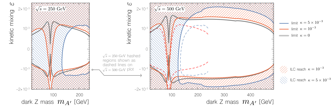
We examine the reach for the ILC to discover the dark in the radiative return channel . The signal rate is strongly enhanced when the photon is collinear with the beam and hence unobservable.44 4 He et al. estimate the discovery reach for a model with pure kinetic mixing at a future lepton collider with cuts that require the photon to be observable [22]. This is overly conservative because a high-mass dimuon resonance is a clean signal whether or not the photon is tagged. We thus calculate the signal as on-shell production at center-of-mass squared energy in the equivalent-particle approximation where the beam of energy contains a distribution of lower-energy particles with energy that account for the unobserved collinear photon of energy [36, 37, 38]. (See Ref. [39] for a pedagogical introduction.) At the leading order in QED perturbation theory, the probability of finding an with energy in the beam is
| (3.10) |
The total signal cross section for is readily expressed in terms of the cross section for two-to-one production of the dark :
| (3.11) |
In the narrow-width approximation, , where is the center-of-mass energy-squared of the “partonic” collision. The cross section for background events mediated by photons or SM bosons follows a similar formula, except that narrow-width approximation does not hold since we will be searching in regions where the photon or are off-shell (unless ). The dark appears as a narrow peak in the dimuon invariant mass distribution. We estimate the signal significance by computing , where is the number of background events in the mass window centered at . The intrinsic width of the dark is very small in the region of interest due to its small couplings. Thus the size of the mass window is controlled by muon momentum resolution. We use [40] in our estimates.
The ILC reach at confidence for a benchmark value of is shown as the colored lines in Fig. 2. This analysis demonstrates that the ILC can serve as the discovery machine for this type of new physics. The ILC reach significantly exceeds both the current limits and the extrapolated sensitivity of the high-luminosity LHC in the kinematically accessible regions. Fig. 5 presents the ILC reach for different values of the mass mixing . We note that for , our results are in agreement with the previous estimates of the dark photon reach in Refs. [19, 41].
Our analysis assumes unpolarized ILC beams. Depending on the model parameters, the couplings of the dark can depend strongly on the lepton chirality, while the background does not have strong polarization dependence. In such models, the appropriate beam polarization may further enhance the ILC reach. However, since the chiral structure of the couplings is not known a priori, running with unpolarized beams is overall the preferred search strategy. If a dark is discovered, polarized beams can be used to measure its chiral couplings; we explore this in the next section.
We also note that, unlike the LHC, hadronic decays of the dark do not suffer from large backgrounds at a lepton collider, and can be included to further improve the ILC reach. We leave this analysis for future work.
4 Precision Measurements at the Dark Pole
Electron–positron colliders such as the ILC are an ideal laboratory to determine the chiral couplings of a dark resonance. This program is analogous to the precision measurements of the electroweak gauge bosons at LEP and SLC. To illustrate this capability, we consider the benchmark point
| (4.1) |
A dark at this benchmark would be already discovered at the HL-LHC, see Fig. 2. Models with slightly smaller couplings may evade the HL-LHC and be first discovered at a 500 GeV ILC. In either case, an electron–positron collider would provide the first opportunity to measure the dark couplings to fermions with high precision, and to determine their chiral structure which is crucial for model discrimination.

The mass of the dark will be measured experimentally at both the HL-LHC and through the radiative return production in the 500 GeV ILC run discussed above. The couplings of the dark may be measured efficiently in a relatively short period of time with a dedicated ILC run at a center-of-mass energy . In this section, we estimate the potential of this run to measure the dark couplings to charged leptons. We study the channel assuming flavor-universal couplings; this assumption is automatically satisfied in our underlying model. The left- and right-handed couplings are defined by
| (4.2) |
and are related to the underlying theory parameters in (2.10); we give numerical values for the benchmark point (4.1). To measure these couplings, we consider three observables:
- •
The number of events,
- •
The forward–backward asymmetry,
- •
The left–right asymmetry for polarized beams, .
The expressions for the two asymmetries are well-known and are summarized in Appendices C and D. The number of events is given by
| (4.3) | ||||
| (4.4) |
Here and denote polarizations of the electron and positron beams, respectively and is the differential luminosity of the colliding beams at the ILC. The somewhat unusual formula for is due to the fact that intrinsic width of the is extremely small, GeV for our benchmark parameters (4.1). The beam luminosity spectrum of the ILC in the vicinity of the nominal center-of-mass energy can be modeled as a Gaussian with a width of order [42], much larger than , as illustrated in Fig. 6. Treating the Breit–Wigner resonance as a -function yields (4.4).
The prediction for depends sensitively on the relative location of the Breit–Wigner resonance with respect to the peak of the luminosity spectrum. To obtain a precise constraint on the couplings from a measurement of , this relative location must be known to a precision GeV. This is a non-trivial requirement. The position of the peak of the luminosity spectrum will be known at the level of MeV [43], which is sufficient. However, prior to the dedicated on-resonance run of the ILC, the mass of the will only be measured as the location of the peak in the dimuon invariant mass distribution, observed either at the HL-LHC or in the radiative-return sample collected at the 500 GeV ILC. In either case, the precision of the mass measurement is limited by the muon momentum resolution, which is of order GeV. A much more precise knowledge of the location of the Breit–Wigner peak is required.
To address this problem, we propose that the on-resonance run of the ILC should begin with an inverse lineshape scan in which the “peak” center-of-mass energy—the location of the peak of luminosity spectrum—is varied in small steps within the mass window inferred from the HL-LHC/ILC-500 data. For example, our benchmark point (4.1) motivates – GeV. At each beam energy step, measure the production cross section. Since the luminosity spectrum is independently known, the can be inferred from the measured cross sections. We estimate that with sufficient statistics at each energy step, this method can provide an error on comparable to the peak beam energy uncertainty, MeV. After performing the inverse lineshape scan, the peak center-of-mass energy can be chosen to match the measured and maximize the dark- production rate.
Fig. 7 shows the expected statistical errors of the measurement of and with one-month and two-month runs on the dark resonance. The ellipses correspond to 95% confidence level measurement, assuming that the best-fit values of the couplings match the underlying model predictions. Also shown are the predictions of three alternative theoretical models of a vector resonance: pure kinetic mixing55 5 The benchmark point is close to the line even though because the contribution of to the chiral couplings is suppressed by . (), mass mixing only (), a parity-conserving (). It is clear from the figure that the measurement of the chiral couplings at the ILC can rule out all three possibilities, establishing parity violation and proving that the underlying dark model has both kinetic and mass mixing. In contrast, the LHC can only constrain the combination , which is not sufficient to discriminate between alternative models.
| Benchmark values | ||
|---|---|---|
| 1 month (unpolarized) | ||
| 1 month (polarized) | ||
| 2 months (polarized) |
The constraint on the couplings inferred from the total number of events is subject to systematic errors from the uncertainties in luminosity and peak beam energy and from the uncertainty in the measurement of the mass . The mass is measured through the inverse lineshape scan. The expected error is of the same order as that in the peak beam energy, MeV. The expected overall luminosity uncertainty is [44]. We estimate that these uncertainties affect the coupling determination at a level that is, at most, comparable to the statistical errors shown in Fig. 7. We do not include uncertainties in the shape of the beam luminosity spectrum. The measurement of the left-right asymmetry is subject to beam polarization uncertainties. ILC polarimeters can achieve a precision of % [45]. The effect of this uncertainty on the coupling measurement is negligible. We collect our estimates of the statistical and combined systematic errors of the chiral coupling measurements in Table 2. We conclude that a dedicated run of the ILC at the dark pole will yield percent-level measurement of and , providing crucial information for discrimination among alternative models of the resonance.
5 Conclusions
A next-generation electron–positron collider, such as the ILC, offers unique opportunities to search for and characterize new physics beyond the Standard Model. In this paper, we study a model of a new Abelian gauge boson, the dark . While SM fermions are not directly charged under the new gauge group, the dark can interact with the SM through both kinetic and mass mixing. If the dark mass is above 10 GeV or so, energy-frontier colliders offer the best way to search for this particle. We studied the current constraints on this particle from precision electroweak measurements and direct searches at the LHC. This extends the previous work on the dark photon model that couples to the SM only via kinetic mixing to the more general case when mass mixing is also present. We evaluate the reach of the ILC, running at 250 and 500 GeV, in the dark parameter space. The ILC reach covers a large part of the parameter space unconstrained by current experiments and not accessible at the HL-LHC; see Fig. 2. Thus, the ILC can serve a discovery machine in this new physics scenario. If a dark is discovered, the ILC offers a unique opportunity to precisely measure its couplings to the SM fermions, including their chiral structure. We demonstrated that a short dedicated run at the center-of-mass energy matching the dark mass will achieve percent-level measurement of the chiral couplings of the dark to leptons. Such a measurement can play a crucial role in model discrimination; this is illustrated in Fig. 7.
The idea of using on-resonance electron-positron collisions to measure the properties of a massive vector boson is, of course, not new: LEP-1 and SLC/SLD used it to understand the Standard Model with unprecedented precision. A new twist in the case of dark is its extremely small intrinsic width, which is much smaller than the width of the beam luminosity spectrum as well as the energy/momentum resolution of the detector for all visible decay products. In this situation, precise measurement of the mass and couplings of the resonance hinges on understanding the beam luminosity spectrum. Note that the small intrinsic width of the dark is directly related to the smallness of its couplings to SM fermions, which is in turn necessary for a sub-TeV resonance to avoid precision electroweak and LHC constraints. Independently of the underlying model, any resonance compatible with current data and kinematically accessible at the ILC will necessarily be very narrow. This motivates further studies of on-resonance production of such narrow states at the ILC and other proposed lepton colliders.
Acknowledgments
We thank Mikael Berggren, Philip Ilten, Gopolang Mohlabeng, Michael Peskin, and Yotam Soreq for insightful discussions. MP and YCS are supported by the National Science Foundation (NSF) grants PHY-1719877 and PHY-2014071. PT is supported by an NSF CAREER award. PT thanks the Aspen Center for Physics (NSF grant #1066293) and Kavli Institute for Theoretical Physics (NSF grant PHY-1748958) for hospitality during a period when part of this work was completed.
Appendix A Simplified Model and Feynman Rules
Our effective dark model is parameterized by the dark mass, , its kinetic mixing to hypercharge, , and a dimensionless –dark mass mixing parameter, . These are related to a benchmark ultraviolet model in Section 2. We use the shorthand , and similarly for cosine, tangent, and the massive gauge boson mixing angle , (2.6).
Mass Spectrum.
The mass spectrum comes from diagonalizing the mass terms (2.4). Assuming , the boson mass to second order in the new physics parameters is
| (A.1) |
where is the order parameter for electroweak symmetry breaking. For completeness, the dark mass is related to the benchmark ultraviolet model parameters to leading order in the new physics parameters by
| (A.2) |
Feynman Rules.
The interactions with Standard Model fermions are described by
| (A.3) |
The effective couplings and charges to leading non-trivial order in and are
| (A.4) | ||||
| (A.5) | ||||
| (A.6) | ||||
| (A.7) |
where according to the SU(2) weight of the left-chiral and is the electric charge. Additional interactions between the , Higgs, and electroweak gauge bosons are not used in this study. The effects are well approximated using the Goldstone boson equivalence theorem, as discussed in Section 2.4. See Ref. [22] for explicit expressions in the pure kinetic mixing case.
Appendix B UV Model and Decoupling Limit
In Section 2.2 we derive our three-parameter model for mass and kinetic mixing as the low-energy theory of an extended Higgs sector. This appendix addresses some model-building aspects of the UV model and connects to known results in the two-Higgs doublet literature.
Decoupling pseudo-Goldstone modes.
There are a total of seven Goldstone modes. Four are eaten by the massive Standard Model gauge bosons and the dark . We decouple the remaining three by adding a trilinear potential that explicitly breaks the global symmetries of the Higgs sector:
| (B.1) |
The scale is assumed to be large compared to the masses in the three-parameter model. The uneaten Goldstones are an orthogonal linear combination to the eaten combination; see Appendix A of Ref. [46].
Decoupling the dark Higgs
. We may tune the potential such that that CP-even state has the largest mass in the UV theory, we define this to be . When integrating out this mode, the trilinear coupling (B.1) generates four-point interactions between the Higgs doublets with a quartic coupling of order . In a given UV model, the perturbativity of the lower-energy two-Higgs doublet theory requires this coupling to be smaller than .
The decoupling limit of the two-Higgs doublet model.
Upon integrating out , our Higgs sector is a CP-conserving two-Higgs doublet model. Gunion and Haber examine the viability of a decoupling limit these models in [47]. In their notation, and and the parameters of their general potential are:
| (B.2) |
The diagonal quadratic and quartic terms are set to produce symmetry-breaking potentials for each of that yield the appropriate vacuum expectation values, and , with mixing angle . The mixing angle encodes the same information as our mass mixing parameter, , (2.5). This potential is manifestly stable in all field directions. The masses for the CP-odd and charged Higgses—the uneaten would-be Goldstones–are
| (B.3) |
The mass matrix between CP-even Higgses is, to leading order in ,
| (B.4) |
where is the quartic coupling for . The rotation to diagonalize the CP-even mass matrix is . The lighter eigenstate is identified with the 125 GeV Higgs boson. The decoupling limit corresponds to the case where an entire SU(2) doublet is heavy. It corresponds to the limit , or . This is readily realized in our model.
Alternative UV completions.
Appendix C Unpolarized Observables
The angular dependence of the differential cross section with spin-averaged beams is
| (C.1) |
where is a kinematic factor independent of the scattering angle of the outgoing muon with respect to the electron beam, . The forward and backward and cross sections are
| (C.2) |
The forward–backward asymmetry is expressed in terms of a coupling asymmetry ,
| (C.3) |
where the superscript on indicates an unpolarized asymmetry.
Appendix D Polarized Beams and Observables
We review the collider phenomenology of polarized beams following the conventions in Ref. [50]. Define the longitudinal electron beam polarization to be where is the number of right (left) helicity particles in the beam. Similarly, let be the analogous quantity for the positron beam. The polarized cross section is related to the pure helicity cross sections and as
| (D.1) |
where we used in the limit of massless fermions coupled to a a vector boson. It is convenient to write this in terms of the symmetric (anti-symmetric) combinations
| (D.2) |
where we note that the spin-averaged (unpolarized) cross section, , is one fourth of .66 6 The unpolarized cross section may be written in terms of helicity cross sections as This gives a compact expression for the polarized cross section in terms of an effective luminosity and an effective polarization
| (D.3) |
The effective polarization is zero for unpolarized beams and for perfectly polarized beams.
The left–right asymmetry for perfectly polarized beams is . For partially polarized beams, we assume that one beam is mostly left-helicity while the other is mostly-right helicity. The cross section the mostly-left helicity electron configuration, , is related to that of the mostly-right helicity electron configuration, , by the replacements and . The left–right asymmetry for the partially polarized beams is
| (D.4) |
where and are the symmetric and antisymmetric combinations of the partially polarized cross sections analogous to (D.2). These are related to the helicity cross sections by
| (D.5) |
One may measure the forward–backward asymmetry for polarized beams. In this case, (C.1) is replaced with
| (D.6) | ||||
| (D.7) |
The resulting forward-backward asymmetry for partially polarized beams is
| (D.8) |
References
- [1] “The International Linear Collider Technical Design Report - Volume 2: Physics,” arXiv:1306.6352 [hep-ph].
- [2] K. Fujii et al., “Physics Case for the 250 GeV Stage of the International Linear Collider,” arXiv:1710.07621 [hep-ex].
- [3] “Physics and Detectors at CLIC: CLIC Conceptual Design Report,” arXiv:1202.5940 [physics.ins-det].
- [4] CLICdp, CLIC Collaboration, T. K. Charles et al., “The Compact Linear Collider (CLIC) - 2018 Summary Report,” arXiv:1812.06018 [physics.acc-ph].
- [5] CEPC Study Group Collaboration, M. Dong et al., “CEPC Conceptual Design Report: Volume 2 - Physics & Detector,” arXiv:1811.10545 [hep-ex].
- [6] FCC Collaboration, A. Abada et al., “FCC Physics Opportunities: Future Circular Collider Conceptual Design Report Volume 1,” Eur. Phys. J. C 79 no. 6, (2019) 474.
- [7] FCC Collaboration, A. Abada et al., “FCC-ee: The Lepton Collider: Future Circular Collider Conceptual Design Report Volume 2,” Eur. Phys. J. ST 228 no. 2, (2019) 261–623.
- [8] I. Kobzarev, L. Okun, and I. Pomeranchuk, “On the Possibility of Experimental Observation of Mirror Particles,” Sov. J. Nucl. Phys. 3 no. 6, (1966) 837–841.
- [9] L. Okun, “Limits of Electrodynamics: Paraphotons?,” Sov. Phys. JETP 56 (1982) 502.
- [10] B. Holdom, “Two U(1)’s and Epsilon Charge Shifts,” Phys. Lett. B 166 (1986) 196–198.
- [11] B. Holdom, “Searching for Charges and a New U(1),” Phys. Lett. B 178 (1986) 65–70.
- [12] R. Foot and X.-G. He, “Comment on Z Z-Prime Mixing in Extended Gauge Theories,” Phys. Lett. B 267 (1991) 509–512.
- [13] H. Davoudiasl, H.-S. Lee, and W. J. Marciano, “’Dark’ Z Implications for Parity Violation, Rare Meson Decays, and Higgs Physics,” Phys. Rev. D 85 (2012) 115019, arXiv:1203.2947 [hep-ph].
- [14] J. Alexander et al., “Dark Sectors 2016 Workshop: Community Report,” 8, 2016. arXiv:1608.08632 [hep-ph].
- [15] M. Battaglieri et al., “Us Cosmic Visions: New Ideas in Dark Matter 2017: Community Report,” in U.S. Cosmic Visions: New Ideas in Dark Matter. 7, 2017. arXiv:1707.04591 [hep-ph].
- [16] M. Fabbrichesi, E. Gabrielli, and G. Lanfranchi, “The Dark Photon,” arXiv:2005.01515 [hep-ph].
- [17] J. L. Feng, A. Rajaraman, and F. Takayama, “Superweakly interacting massive particles,” Phys. Rev. Lett. 91 (2003) 011302, arXiv:hep-ph/0302215.
- [18] D. Curtin, R. Essig, S. Gori, and J. Shelton, “Illuminating Dark Photons with High-Energy Colliders,” JHEP 02 (2015) 157, arXiv:1412.0018 [hep-ph].
- [19] M. Karliner, M. Low, J. L. Rosner, and L.-T. Wang, “Radiative return capabilities of a high-energy, high-luminosity collider,” Phys. Rev. D 92 no. 3, (2015) 035010, arXiv:1503.07209 [hep-ph].
- [20] S. Gopalakrishna, S. Jung, and J. D. Wells, “Higgs Boson Decays to Four Fermions Through an Abelian Hidden Sector,” Phys. Rev. D 78 (2008) 055002, arXiv:0801.3456 [hep-ph].
- [21] J. Liu, X.-P. Wang, and F. Yu, “A Tale of Two Portals: Testing Light, Hidden New Physics at Future Colliders,” JHEP 06 (2017) 077, arXiv:1704.00730 [hep-ph].
- [22] M. He, X.-G. He, C.-K. Huang, and G. Li, “Search for a heavy dark photon at future colliders,” JHEP 03 (2018) 139, arXiv:1712.09095 [hep-ph].
- [23] J. M. Cornwall, D. N. Levin, and G. Tiktopoulos, “Derivation of Gauge Invariance from High-Energy Unitarity Bounds on the s Matrix,” Phys. Rev. D 10 (1974) 1145. [Erratum: Phys.Rev.D 11, 972 (1975)].
- [24] M. S. Chanowitz and M. K. Gaillard, “The TeV Physics of Strongly Interacting W’s and Z’s,” Nucl. Phys. B 261 (1985) 379–431.
- [25] CMS Collaboration, A. M. Sirunyan et al., “Search for a Narrow Resonance Lighter than 200 GeV Decaying to a Pair of Muons in Proton-Proton Collisions at TeV,” Phys. Rev. Lett. 124 no. 13, (2020) 131802, arXiv:1912.04776 [hep-ex].
- [26] CMS Collaboration, A. M. Sirunyan et al., “Search for resonant and nonresonant new phenomena in high-mass dilepton final states at = 13 TeV,” JHEP 07 (2021) 208, arXiv:2103.02708 [hep-ex].
- [27] ATLAS Collaboration, G. Aad et al., “Search for high-mass dilepton resonances using 139 fb-1 of collision data collected at 13 TeV with the ATLAS detector,” Phys. Lett. B 796 (2019) 68–87, arXiv:1903.06248 [hep-ex].
- [28] G. D. Kribs, D. McKeen, and N. Raj, “Breaking up the Proton: An Affair with Dark Forces,” Phys. Rev. Lett. 126 no. 1, (2021) 011801, arXiv:2007.15655 [hep-ph].
- [29] B. Yan, “Probing the dark photon via polarized DIS scattering at the HERA and EIC,” arXiv:2203.01510 [hep-ph].
- [30] S. Kanemura, T. Moroi, and T. Tanabe, “Beam dump experiment at future electron–positron colliders,” Phys. Lett. B 751 (2015) 25–28, arXiv:1507.02809 [hep-ph].
- [31] K. Asai, S. Iwamoto, Y. Sakaki, and D. Ueda, “New physics searches at the ILC positron and electron beam dumps,” JHEP 09 (2021) 183, arXiv:2105.13768 [hep-ph].
- [32] Particle Data Group Collaboration, P. Zyla et al., “Review of Particle Physics,” PTEP 2020 no. 8, (2020) 083C01. See Section 10, Electroweak Model and Constraints on New Physics.
- [33] A. Hook, E. Izaguirre, and J. G. Wacker, “Model Independent Bounds on Kinetic Mixing,” Adv. High Energy Phys. 2011 (2011) 859762, arXiv:1006.0973 [hep-ph].
- [34] D. B. Clark, E. Godat, and F. I. Olness, “ManeParse : A Mathematica reader for Parton Distribution Functions,” Comput. Phys. Commun. 216 (2017) 126–137, arXiv:1605.08012 [hep-ph].
- [35] K. Kovarik et al., “nCTEQ15 - Global analysis of nuclear parton distributions with uncertainties in the CTEQ framework,” Phys. Rev. D 93 no. 8, (2016) 085037, arXiv:1509.00792 [hep-ph].
- [36] C. F. von Weizsacker, “Radiation emitted in collisions of very fast electrons,” Z. Phys. 88 (1934) 612–625.
- [37] E. J. Williams, “Correlation of certain collision problems with radiation theory,” Kong. Dan. Vid. Sel. Mat. Fys. Med. 13N4 no. 4, (1935) 1–50.
- [38] M.-S. Chen and P. M. Zerwas, “Equivalent-Particle Approximations in electron and Photon Processes of Higher Order QED,” Phys. Rev. D 12 (1975) 187.
- [39] M. Perelstein, “Introduction to Collider Physics,” in Theoretical Advanced Study Institute in Elementary Particle Physics: Physics of the Large and the Small, pp. 421–486. 2011. arXiv:1002.0274 [hep-ph].
- [40] H. Abramowicz et al., “The International Linear Collider Technical Design Report - Volume 4: Detectors,” arXiv:1306.6329 [physics.ins-det].
- [41] ILD concept group Collaboration, C. M. Berggren, “New physics searches with the ILD detector at the ILC,” PoS PANIC2021 (2022) 123, arXiv:2111.09928 [hep-ex].
- [42] F. Simon, “Perspectives for Top Quark Physics at the (I)LC,” in 7th International Workshop on Top Quark Physics. 11, 2014. arXiv:1411.7517 [hep-ex].
- [43] N. Muchnoi, H. J. Schreiber, and M. Viti, “ILC Beam Energy Measurement by means of Laser Compton Backscattering,” Nucl. Instrum. Meth. A 607 (2009) 340–366, arXiv:0812.0925 [physics.ins-det].
- [44] I. Božović Jelisavčić, S. Lukić, G. Milutinović Dumbelović, M. Pandurović, and I. Smiljanić, “Luminosity measurement at ILC,” JINST 8 (2013) P08012, arXiv:1304.4082 [physics.acc-ph].
- [45] S. Boogert et al., “Polarimeters and Energy Spectrometers for the ILC Beam Delivery System,” JINST 4 (2009) P10015, arXiv:0904.0122 [physics.ins-det].
- [46] I. Chaffey and P. Tanedo, “Vector self-interacting dark matter,” Phys. Rev. D 101 no. 7, (2020) 075005, arXiv:1907.10217 [hep-ph].
- [47] J. F. Gunion and H. E. Haber, “The CP conserving two Higgs doublet model: The Approach to the decoupling limit,” Phys. Rev. D 67 (2003) 075019, arXiv:hep-ph/0207010.
- [48] E. C. G. Stueckelberg, “Interaction Energy in Electrodynamics and in the Field Theory of Nuclear Forces,” Helv. Phys. Acta 11 (1938) 225–244.
- [49] D. Feldman, Z. Liu, and P. Nath, “The Stueckelberg Z-Prime Extension with Kinetic Mixing and Milli-Charged Dark Matter from the Hidden Sector,” Phys. Rev. D 75 (2007) 115001, arXiv:hep-ph/0702123.
- [50] G. Moortgat-Pick et al., “The Role of polarized positrons and electrons in revealing fundamental interactions at the linear collider,” Phys. Rept. 460 (2008) 131–243, arXiv:hep-ph/0507011.