- IRS
- Intelligent reflecting surface
- RIS
- reconfigurable intelligent surface
- irs
- intelligent reflecting surface
- PARAFAC
- parallel factor analysis
- TALS
- trilinear alternating least squares
- DF
- decode-and-forward
- AF
- amplify-and-forward
- CE
- channel estimation
- RF
- radio-frequency
- THz
- Terahertz communication
- EVD
- eigenvalue decomposition
- CRB
- Cramér-Rao lower bound
- CSI
- channel state information
- BS
- base station
- MIMO
- multiple-input multiple-output
- NMSE
- Normalized Mean Square Error
- 2G
- Second Generation
- 3G
- 3 Generation
- 3GPP
- 3 Generation Partnership Project
- 4G
- 4 Generation
- 5G
- 5 Generation
- 6G
- 6 generation
- E-TALS
- enhanced TALS
- UT
- user terminal
- LS
- least squares
Semi-Blind Joint Channel and Symbol Estimation for IRS-Assisted MIMO Systems
Abstract
IRS (IRS) is a promising technology for the 6G of wireless systems, realizing the smart radio environment concept. In this paper, we present a novel tensor-based receiver for IRS-assisted MIMO communications capable of jointly estimating the channels and the transmitted data streams in a semi-blind fashion. Assuming a fully passive IRS architecture and introducing a simple space-time coding scheme at the transmitter, the received signal model can be advantageously built using the PARATUCK tensor model, which can be seen as a hybrid of PARAFAC and Tucker models. Exploiting the algebraic structure of the PARATUCK tensor model, a semi-blind receiver is derived. The proposed receiver is based on a trilinear alternating least squares method that iteratively estimates the two involved – IRS-BS and UT-IRS – communication channels and the transmitted symbol matrix. We discuss identifiability conditions that ensure the joint semi-blind recovery of the involved channel and symbol matrices, and propose a joint design of the coding and IRS reflection matrices to optimize the receiver performance. For the proposed semi-blind receiver, the derivation of the expected CRB is also provided. A numerical performance evaluation of the proposed receiver design corroborates its superior performance in terms of the normalized mean squared error of the estimated channels and the achieved symbol error rate.
Index Terms:
Intelligent reflecting surface, channel estimation, symbol estimation, MIMO, tensor modeling, PARATUCK, semi-blind receiver.I Introduction
IRS or RIS is a promising technology for 6G (6G) wireless systems [1]. An IRS consists of a two-dimensional array of a large number of passive or semi-passive elements, each of which can independently and dynamically tune the desired phase shift and amplitude of the incident radio waves [2, 3]. An immediate and simplified application of IRS is to overcome the blockage problem between the transmitter and intended receivers in wireless networks, which reduces the dead zone11 1 Although a dead zone can be surpassed using relay technology, an IRS can be more advantageous in terms of cost since, as opposed to AF (AF) or DF (DF) relays that require a dedicated power source, IRS does not require power-hungry radio-frequency chains and can also be wirelessly powered by an external RF-based source [4]. The key differences and similarities between IRS and relays are discussed in [5]. [6]. Due to its ability to shape the propagation environment, IRS can be employed in various scenarios to achieve several other goals as well, as it is discussed in [7]. However, deploying IRS in wireless communication systems involves a number of challenges, including CSI (CSI) acquisition [3, 8, 9].
Acquiring CSI is an important issue, since the accuracy of the channel estimate has a direct impact on the gains obtained by IRS-assisted communications. The difficulty is in part due to the passive nature of the surface and the high number of reconfigurable elements. Recent works have proposed CE (CE) methods to IRS-assisted communications. These works can be classified according to the IRS architecture, system setup and signal processing methodology [10]. For example, regarding the IRS architecture, it can be assumed that the IRS is fully passive, i.e., it does not have signal processing capabilities and cannot send/process pilot sequences, as it was pointed out in [11], which investigates CE in the context of IRS-assisted THz. Alternatively, the IRS can be semi-passive, where some IRS elements are equipped with a few RF (RF) chains to facilitate the CE, as in [12].22 2 Note that a fully passive architecture is more challenging, since the estimation of the cascaded channel, TX-IRS-Rx, or the individual channels Tx-IRS and IRS-Rx channels should be carried out at the receiver or transmitter.
In the system setup category, single and multiuser systems – depending on whether the communication links are assisted by a single or multiple IRS – can be distinguished. As an example, the authors in [13] and [14] consider a multiuser system, and the CE solution is based on an anchoring scheme, where two nodes are positioned near the IRS in order to aid the BS (BS). Also, references [15, 16, 17, 18] propose CE strategies, in which multi-stage or multi-time scale estimation techniques are exploited. A double IRS-assisted system is considered in [19], in which CE and a passive beamforming design are investigated.
Recently, several mechanisms based on deep learning and compressed sensing to acquire CSI have been proposed [20, 21]. The conventional LS (LS) CE is assumed in [22], where a minimum variance unbiased estimator is proposed. In [23], channel training is divided into blocks. Each block provides a partial channel estimate in the LS sense, so that the total channel matrix is accomplished once all blocks are processed. Paper [24] proposes a matrix factorization method based on EVD (EVD). A tensor based solution for IRS-assisted MIMO (MIMO) systems is proposed in [25]. That method relies on a PARAFAC (PARAFAC) modeling of the received signals. It is shown that decoupled estimates of the involved MIMO communication channels can be obtained iteratively or in closed form. The works [26] and [27] also exploit tensor modeling to solve the CE task in IRS-assisted downlink multi-user systems. The use of tensor methods has been investigated in several previous works in the context of point-to-point [28, 29, 30, 31] and cooperative (relay-assisted) MIMO systems [32, 33, 34]. The success of tensor-based methods comes from the powerful uniqueness properties of tensor decompositions compared to matrix-based ones. Moreover, in wireless communications, tensor-based algorithms efficiently exploit the multi-dimensional nature of the received signals in the time, space, and frequency domains. This multi-dimensional characterization of the received signals leads to more flexible transceiver designs than those offered by conventional matrix-based solutions. Recognizing these benefits of tensor-based algorithms, this paper takes a different approach compared to previous works, and provides joint estimates of the involved communication channels and the transmitted symbols in a semi-blind fashion.
Assuming a fully passive surface architecture and introducing a simple space-time coding scheme at the transmitter, we recast the received signal as a PARATUCK tensor model, which can be seen as a hybrid of PARAFAC and Tucker models [35, 36, 37, 38]. Exploiting the algebraic structure of the PARATUCK tensor model, namely, the different matrix unfoldings of the received signal tensor, a semi-blind receiver based on a TALS (TALS) estimation scheme is proposed. Our receiver design iteratively estimates the two involved (IRS-BS and UT (UT)-IRS) communication channels and the symbol matrix. Moreover, by resorting to the identifiability results of the PARATUCK tensor model, we derive useful system design recommendations that ensure the joint semi-blind recovery of the involved channel and the symbol matrices. In particular, we propose a joint design of the coding matrix and the IRS reflection matrix to optimize the receiver performance. We also present an extension of the proposed receiver algorithm to a scenario, in which the direct link is available. In this scenario, an initial estimation of the transmitted symbol matrix obtained from the direct link is used as a warm start to enhance the semi-blind joint channel and symbol estimation via the IRS-assisted link. Finally, we provide expressions for the expected CRB (CRB) for the proposed semi-blind receiver.
In the following, we summarize the main contributions of this work.
- •
We present a novel tensor-based semi-blind receiver algorithm for IRS-assisted MIMO systems that avoids the a priori training phase. The proposed algorithm iteratively estimates the two involved channel matrices as well as the symbol matrix by means of a TALS algorithm, which exploits a PARATUCK tensor model for the received signals.
- •
We extend the proposed semi-blind receiver to a scenario, in which the direct link between transmitter and receiver is available. In this case, the receiver processing has two stages. In the first one, an initial semi-blind estimate of the transmitted symbols obtained via the direct link is used as a warm start of the joint channel and symbol estimation via the IRS-assisted link.
- •
We derive conditions for the joint channel and symbol identifiability, and discuss the design of the coding matrix and the IRS phase shift matrix. A joint design is proposed to improve the receiver performance.
- •
We investigate the impact of the direct channel estimation on the accuracy of the IRS-assisted channel estimation, showing that a good estimate of the direct channel in the first stage improves the performance of the joint channel and symbol estimate in the second stage.
- •
We derive the expected CRB for the proposed TALS-PARATUCK semi-blind receivers, allowing to study its performance analytically.
Notation and properties: Matrices are represented with boldface capital letters (, and vectors are denoted by boldface lowercase letters (. Tensors are symbolized by calligraphic letters . Transpose and pseudo-inverse of a matrix are denoted as and , respectively. is a diagonal matrix holding the th row of on its main diagonal. The operator forms a diagonal matrix out of its vector argument, while , , , and denote the conjugate, outer product, Khatri Rao, Hadamard and Kronecker products, respectively. denotes the identity matrix. The operator vectorizes an matrix argument, while does the opposite operation. Moreover, forms a vector out of the diagonal of its matrix argument. ¨The -mode product between a tensor and a matrix is denoted as , for . An identity -way tensor of dimension is denoted as . Moreover, and denotes the -th row and -th column of the matrix , respectively. The operator rounds its fractional argument up to the nearest integer. In this paper, we make use of the following identities:
| (1) |
| (2) |
| (3) |
If is a diagonal matrix, we have:
| (4) |
II Tensor preliminaries
In this section, we provide a brief overview on two tensor decompositions that are of interest to this work, namely the PARAFAC and PARATUCK decompositions. They will be exploited in the formulation of the proposed receivers. In order to keep the presentation concise, the focus is on the key definitions and expressions used to represent these two tensor decompositions.
II-A PARAFAC decomposition
The PARAFAC decomposition, also known as the canonical polyadic decomposition (CPD), is the most popular tensor decomposition, which expresses a tensor as a sum of a minimum number of rank-one tensors [39, 40, 41, 42]. For a third-order tensor , its scalar form and frontal slice representation is given as
| (5) |
and
| (6) |
respectively, where denotes the -th entry of the tensor and is the -th frontal slice (a.k.a. as -mode slice) of the tensor , for . The scalars , and are corresponding entries of the three factor matrices , , and , while denotes the rank of the tensor . where is the -th frontal slice (a.k.a. as 3-mode slice) of the tensor , . The PARAFAC decomposition is powerful due to its essential factor identification uniqueness property, which has its roots on the concept of the Kruskal rank (k-rank). Further details can be found in [43, 44].
II-B PARATUCK decomposition
The PARATUCK decomposition [37, 45] is a hybrid tensor decomposition that combines the Tucker [46] and the PARAFAC decompositions. It enjoys the powerful uniqueness properties of the PARAFAC model, while offering a more flexible structure by allowing controlled interactions among its factor matrices. Its scalar form and frontal slice representations are given as
| (7) |
and
| (8) |
respectively, where , , , and are the elements of the matrices , , , and , respectively. and are referred to as the factors matrices, and are the interactions matrices, while is the core matrix, whose -th entry defines the level of interaction between the -th column of and the -th column of .
III System Model

Let us consider a MIMO communication system assisted by an IRS, where the BS and UT have arrays of and antennas, respectively, while the IRS is composed of elements, which can be individually adjusted/configured to generate phase shifts. We assume a two-stage structured time-domain transmission, as illustrated in Fig. 1, where the estimation time is split into blocks, and each block has symbol periods each, with . We focus on the uplink scenario, where a multi-antenna UT encodes independent data streams that are received at the BS with the assistance of an IRS, and possibly reach the BS directly (if the direct link is available).33 3 Although the uplink case is assumed here, the signal model and the algorithms proposed in this paper are equally applicable to the downlink case by just inverting the roles of the transmitter and the receiver.
In the general case (when the direct link available), the discrete-time baseband received signal vector during the -th symbol period of the -th block is given by
| (9) |
where is the direct channel matrix between the UT and the BS, whereas and denotes the IRS-BS and UT-IRS channel matrices, respectively. The UT employs a space-time encoding scheme that “diagonally” encodes the input symbols such that contains the encoded symbol vector, , transmitted during the -th symbol period of the -th block. The vector collects the IRS phase shifts, and is the corresponding additive white Gaussian noise vector. We assume that the phase shift vector and the coding vector are constant during the time slots of the -th block, and vary from block to block, which means that and , for .
With these assumptions, collecting the received signals during the time slots of each block yields
| (10) |
where collects the received signal vectors during the time slots of the -th block. In this paper, we consider two possible scenarios. In the first one, the direct link is assumed to be weak, or unavailable. In the second one, both the IRS-assisted link and the direct link are exploited.
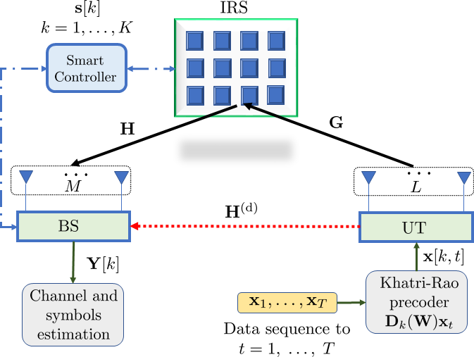

Regarding the channel model, no particular assumption is made in this paper. We can assume that the channel matrices follow an i.i.d Rayleigh fading model, or, alternatively, are described by a geometrical model with a few specular paths. For instance, we can assume that the UT-IRS and IRS-BS links are subject to low scattering propagation, such that , and , where , , and are the array response matrices, and the vectors and hold the complex amplitude coefficients of the IRS-BS and UT-IRS channels, respectively, while and denote the number of clusters between IRS-BS and UT-IRS, respectively [47].
IV Semi-blind receiver without the direct link
Considering the first scenario, when the direct link is weak or unavailable, the received signal in (10) reduces to
| (11) |
where , are the phase shift matrix and coding matrix, respectively, and is the transmitted symbol matrix. Note that the useful (signal) part of the received signal during the -th block can be identified as the -th matrix slice of a received signal tensor that satisfies a PARATUCK decomposition [36, 37], where the scalar form of the noiseless received signal tensor can be expressed as
| (12) |
Note that the interaction matrices of the PARATUCK model correspond to the matrices and that collect, respectively, the phase shifts (introduced by the IRS) and the coding coefficients (applied at the transmitter), which are fixed and known at the receiver. To summarize, comparing equations (8) and (11), the following correspondence can be established
| (13) |
The algebraic properties of this PARATUCK tensor signal model will be exploited to formulate our semi-blind receiver for joint channel and symbol estimation. A more complete scenario, in which the direct link is available, as indicated in (10), will be discussed later.
Remark 1
The IRS-assisted channel is usually represented in an equivalent form in which the channels and are linked by a Khatri-Rao product. This link can be seen by defining the channel parameter vector . In general, can be directly estimated in the LS sense from the received signal, or constructed once the individual estimates of and are obtained. In this paper, we adopt the second approach.
Our goal is to jointly estimate all the UT-IRS channel , the IRS-BS channel , and the symbol matrix by exploiting the tensor structure of the received signal model (11). We start by stating the following optimization problem:
| (14) |
Clearly, this problem is highly nonlinear, since it involves multiple products of the unknown variables, represented by the matrices , and . However, we take a simpler route to solve the above problem by capitalizing on the multi-linear nature of the received signal and exploiting the PARATUCK tensor model structure [36, 37]. By operating on each one of the three different matrix unfoldings of this tensor model, we derive the key equations for conditionally minimizing the cost function (14) with respect to each unknown matrix in the least squares (LS) sense, while assuming that the remaining quantities are fixed. To simplify the presentation, we temporarily omit the noise term during the development of the main steps.
IV-A Estimation of the IRS-BS channel
Let us first consider the estimation of the IRS-BS channel matrix. Starting from the frontal slice representation in (11), and stacking column-wise the matrix slices , , we get
| (15) |
which corresponds to the 1-mode unfolding of the received signal tensor in (12), where
| (16) |
and is the corresponding 1-mode unfolding of the additive noise tensor. The estimation of can be obtained by solving the following LS problem
| (17) |
the solution of which is given by
| (18) |
IV-B UT-IRS channel estimation
To derive the update equation for the estimation of the UT-IRS channel matrix , let us apply the operator to (11), which gives
| (19) | ||||
where we have applied property (2) twice. Now, applying property (3) to (19) yields
| (20) |
where we have used the fact that is actually . By stacking column-wise , and using (20), we can obtain the 3-mode unfolding of the received signal tensor as follows
| (21) | ||||
where
| (22) | ||||
Finally, vectorizing (21) and applying property (2) yields
| (23) |
Thus, an estimate of in the LS sense can be obtained by solving the following problem
| (24) |
the solution of which is given by
| (25) |
Remark 2
The step 2 of Algorithm 1, which is concerned with the estimation of the UT-IRS channel matrix, can be simplified by assuming that defined in (22) is an semi-unitary matrix satisfying (this choice is discussed in Appendix B). In this case, it can be shown that the LS estimation step (25) simplifies to
| (26) |
where , and
| (27) |
In addition to the complexity reduction, our numerical experiments have shown that the semi-unitary design for also improves the convergence speed of Algorithm 1. On the other hand, this condition requires . It is worth noting, however, that although advantageous from a performance/complexity viewpoint, the semi-unitary condition is not necessary.
input : ; Initialize and
- 1.
Using and compute
from (16) and find
a least squares estimate of : - 2.
Using and , find
a least squares estimate of : - 3.
Using and compute
from (29) and find
a least squares estimate of : - 4:
- 5:
Repeat steps to until convergence.
IV-C Symbol estimation
The final step of our semi-blind receiver estimates the transmitted symbol matrix. To this end, we start from (11), and stack column-wise the matrix slices , to get
| (28) |
which corresponds to the 2-mode unfolding of the received signal tensor in (12), where
| (29) |
Adding the noise term, we have . The LS estimate of is then obtained by solving
| (30) |
the solution of which is given by
| (31) |
The proposed semi-blind receiver makes use of (18), (26) and (31) to obtain the estimates of channel matrices and , and the symbol via a trilinear alternating least squares based estimation scheme, herein referred to as TALS receiver. More specifically, the algorithm consists of a three-step estimation procedure that estimates one matrix at each step, while fixing the other two matrices to their values obtained at the previous estimation steps. Note that the proposed TALS receiver is a semi-blind method, since no training sequences are required. The receiver algorithm is summarized in Algorithm 1.
The stopping criterion relies on the normalized squared error measure computed at the end of the -th iteration, given by , where . The convergence is declared when the difference between the reconstruction errors of two successive iterations falls below a threshold, i.e., . In this work, we assume . The convergence criterion of TALS is based on the difference between the reconstruction errors computed in two successive iterations. The complexity of the TALS receiver is dominated by the matrix inverses in steps and , which have complexity orders and , respectively [35]. Considering the complexity of step 2, which only involves matrix products, the total complexity by iteration of the TALS receiver is given by .
IV-D Identifiability
The joint recovery of , , and requires that the three LS problems in (17), (24), and (30), have unique solutions, respectively. More specifically, the uniqueness of requires that defined in (16) have full column-rank, which implies , while the uniqueness of requires that have full column-rank, implying . Likewise, the uniqueness of requires that defined in (29) be of full column-rank, which implies . Note that the number of transmitted blocks is the common parameter in these three conditions, which must be simultaneously satisfied. In summary, the following conditions must be simultaneously satisfied the joint uniqueness of , , and :
| (32) |
These conditions establish useful trade-offs involving the time diversities (parameters and ) and spatial diversities (parameters , , ) for the joint recovery of the channel and symbol matrices. More specifically, reducing the number of blocks and/or the number of symbol periods can be compensated by a corresponding increase on the number of BS antennas . As a special case, if the number of BS antennas exceeds the number of UT antennas (), satisfying these conditions reduces to .
Under the conditions stated above, the estimates of , , and delivered by Algorithm 1 are affected by scaling ambiguities that compensate each other, as follows
| (33) |
where , , and are diagonal matrices. These scaling ambiguities can be handled by assuming that the first row of the symbol matrix contains identification symbols that are known at the receiver. Note that the columns of correspond to the data streams that are spatially multiplexed at the transmitter. Hence, the knowledge of the first row of means that the first symbol of each data stream is a known pilot. Therefore, the knowledge of pilots allows us to eliminate the scaling ambiguity by normalization. A simple choice is to assume that , so that can be determined from the first row of the estimated symbol matrix after convergence of Algorithm 1, and cancelled out by normalization.
Remark 3
The identifiability conditions (32) show that the minimum value of can be small if the block length is large. However, this minimum value may not be enough to obtain a fine CE estimate, especially when the number of IRS elements is large. In this case, must be increased to ensure a good performance. To overcome this practical challenge, we can resort to alternative strategies proposed in the literature, such as the partitioning of the IRS panel into multiple sub-panels [48, 26]. As an example, for an IRS consisting of elements and partitioned into sub-panels, the minimum value of that ensures identifiability according to (32) is reduced by a factor of 10, for fixed values of and , leading to an increased spectral efficiency. In this case, the proposed semi-blind receiver is run independently and in parallel for each sub-panel. Moreover, if the elements within a given sub-panel are spatially correlated, one can assume the same phase shift for the entire sub-panel and further reduce . Consequently, each sub-panel is associated with one aggregated channel coefficient (see, e.g. [10]) for further details on this strategy.
V Direct link aided Semi-Blind Receiver

In this section, we present an enhanced version of the semi-blind receiver derived in the previous section that exploits the direct link between UT and BS, whenever it is available. The idea is to dedicate part of the transmission time resources to the direct link, so that an initial estimate of the transmitted symbols and direct channel can be obtained. The initial symbol estimates are exploited as a “warm start” of the TALS algorithm for estimating the UT-IRS and IRS-BS channels, while refining the estimates of the symbols and the direct channel. To this end, we slightly modify the transmission protocol by splitting the total transmission time of blocks into two time windows of duration and symbol periods, respectively, where is the total number of time blocks, and the total transmission duration. The time protocol is depicted in Figure 4. During the first time window, the UE transmits data using a coding matrix , while in the second time window it uses the coding matrix and the phase shift matrix . A short discussion on the design of and is provided in the Appendix B.
The receiver processing has two stages. In the first one, a joint estimation of the direct channel and the transmitted symbols is carried out during the first time window by exploiting the PARAFAC tensor model of the received signals. The second stage makes use of the estimated symbols in the first time window as an initialization of the TALS algorithm that jointly estimates the involved channel matrices, while refining the symbol estimates during its iterative process. As will be shown later in our numerical experiments, the initialization of the IRS-assisted link using the direct link estimates yields an enhanced TALS algorithm with accelerated convergence and improved estimation accuracy. Therefore, in stage one the IRS is “off”, following the approach of [14], so that the received signal at BS is given as
| (34) |
for , where is the coding matrix used during the first time window of blocks. The signal part of (34) can be viewed as the -th frontal matrix slice of a three-way tensor that follows a PARAFAC decomposition with factor matrices . By analogy with (6), the following correspondences can be deduced:
| (35) |
From the uniqueness property of the PARAFAC model [43, 44], one can obtain a useful condition for guaranteed direct channel and symbol recovery in the general case where all the factor matrices of are unknown. In our context, however, since the coding matrix is assumed to be known at the receiver (BS), simplified conditions can be obtained. Since has full column-rank (which requires ), receive antennas and time slots are enough for the joint recovery of and . This problem can be efficiently solved by means of the Khatri-Rao Factorization algorithm [25], as will be detailed next.
V-A Stage I: Joint direct channel and symbol estimation
Starting from (34), and defining
| (36) |
that collects the signals received during the first time blocks, we have
| (37) |
where we have used property (4), and is the corresponding noise matrix. Defining
an estimate of and can be found using the Khatri-Rao Factorization algorithm that solves the following problem [49, 50]
| (38) |
which is equivalent to solving rank- matrix approximation subproblems, and can be stated as
| (39) |
where , and denotes the -th column of , while and are the -th column of and -th row of , respectively. Due to space limitations, we have suppressed the details of the KRF algorithm. A pseudo code of this algorithm can be found in [25].
Remark 4
As an alternative to the KRF algorithm, one can also resort to the bilinear alternating least squares (BALS) algorithm that jointly estimates the direct channel matrix and the symbol matrix in an alternating way. In this work, we advocate using the KRF algorithm since it provides similar performance to BALS, while being a closed-form solution that affords an efficient implementation, since the involved rank-one matrix approximations can be optimized if executed in a parallel processing hardware.
V-B Stage II: IRS-assisted channel estimation and symbol refinement
After the stage I, the IRS is turned “on” during the second transmission time window that spans blocks. In this case, the total received signal is given by the sum of the direct link and IRS-assisted contributions, and is given by
| (40) | |||||
From the estimated symbol and direct channel matrices and delivered by the KRF algorithm in stage I (c.f. problem (39)), the interference form the direct link can be removed (or minimized) by subtracting an estimate of its contribution from the total received signal in stage II, yielding
| (41) |
From (40), we can write (41) as
| (42) |
where is the effective noise, while and are error matrices associated with the estimates of the direct channel and symbol matrix in stage I. It is clear that the energy of the overall additive noise term in (41) will depend on the energy of these error terms, which in turn depends on the quality of the direct link compared with the IRS-assisted link.
Note that the signal part of (42) corresponds to a PARATUCK decomposition of , which is analogous to the (11), where the third mode has dimension (instead of ). Hence, estimates of the IRS-assisted channel matrices and , as well as refined estimates of the symbol matrix can be obtained from by following the procedure discussed in Section IV.A-IV.C. This leads to a second semi-blind receiver, referred to as E-TALS (E-TALS), summarized in Algorithm 2.
In addition, from the refined symbol estimates, an enhanced estimate of the direct channel matrix can also be obtained at the end of stage II, i.e., at the convergence of the algorithm. More specifically, suppose that the E-TALS algorithm has converged at the -th iteration, and let be the refined estimate of the symbol matrix obtained at the this iteration. Substituting into (34), a refined estimate of the direct channel can be obtained by solving the following problem
| (43) |
the solution of which is given by
| (44) |
In summary, when the direct link is available, the proposed E-TALS receiver allows not only to improve the convergence speed of stage II by using previous symbol estimates as a “warm start”, but also allows to continuously improve the accuracy of these symbol estimates via the IRS-assisted link, while enhancing the estimate of the involved channel matrices, including the direct channel matrix. As will be clear from our numerical experiments, the availability of the direct link makes E-TALS (Algorithm 2) advantageous compared to TALS without the availability of the direct link (Algorithm 1).
Note that the identifiability condition discuss to TASL it is valid for E-TALS algorithm 2 with an additional restriction, which consist in is required due the proposed KRF solution in first stage.
output : , , , and
- 1.
From , compute
and from the KRF algorithm
input : i = 0; initialize ,
- 2.
- 3.
- 4.
Repeat steps and until convergence.
- 5:
From the refined estimate , compute a final estimate
of the direct link channel:.
VI Numerical Results
We evaluate the performance of the proposed semi-blind receivers. The CE accuracy is evaluated in terms of the normalized mean square error (NMSE) given by
| (45) |
where and denotes the estimation of the channels at the -th run, and denotes the number of Monte-Carlo runs. The same definition applies to the estimated UT-IRS channel. We also evaluate the symbol error rate (SER) performance as a function of the signal to noise ratio (SNR) defined as , where is the noiseless received signal tensor generated according (12), and is the additive noise tensor. All the results represent an average from at least Monte Carlo runs. Each run corresponds to an independent realization of the channel matrices, transmitted symbols and noise term. Regarding the channel model, we consider the Rayleigh fading case (i.e. the entries of channel matrices are independent and identically distributed zero-mean circularly-symmetric complex Gaussian random variables) as well as the geometrical channel model with a few specular paths, as described in Section II. We assume uniform linear arrays at the BS and UT, while the IRS panel has a uniform rectangular array structure. The transmitted symbols follow a 16-PSK constellation. When considering the direct link, we define as the effective SNR gap (in dB) between direct link and the IRS-assisted link. Otherwise stated, the average received signal power for the direct link is dB smaller than that of the IRS-assisted link. In Figures 5-7, we assume that the direct link is blocked and focus on the TALS receiver (Algorithm 1), while in the remaining figures the direct link is available and both TALS and E-TALS are considered.
VI-A TALS performance: NMSE, CRB and SER
In Figure 5, we evaluate the NMSE performance of the semi-blind TALS receiver, while comparing it with competing CE methods. We consider as references for comparisons the Block-LS44 4 The competing CE method of [23] has two stages. In the first one, the cascaded channel associated with each time block is individually estimated via an LS method, while in the second stage the path angles are extracted from the unstructured channel estimates. Since our semi-blind receiver in not concerned with the extraction of the angular parameters of the channel matrices (which can be done using existing methods), we compare the proposed TALS method with the first stage of the Block-LS method of [23]. CE method of [23] and the pilot-assisted PARAFAC-BALS method proposed in [25]. Both methods are direct competitors since they operate on the same system model as the proposed semi-blind receiver. The second is based on an iterative estimation of the UT-IRS and IRS-BS channel matrices using a BALS algorithm. However, the main difference is on the fact that these methods require the transmission of pilot sequences, while the proposed receiver jointly estimate the channel and the transmitted symbols semi-blindly. In this experiment, we assume antennas at the BS, antennas at the UT, and an IRS composed of reflecting elements. The total transmission time consists of blocks of time slots each. The channel matrices associated with the IRS-BS and UT-IRS are generated according to a geometrical channel model, assuming a single path scenario (line of sight case). The path directions are randomly generated according to a uniform distribution. At each Monte Carlo run, the azimuth and elevation angles are drawn within the intervals and , respectively.
As it can be seen from the figure, the TALS receiver offers a more accurate overall channel estimate than Block-LS and PAFAFAC-BALS. In particular, the Block-LS method has an SNR gap of approximately dB compared to TALS. Indeed, the TALS receiver fully exploits the trilinear structure of the received signal, and its improved performance comes from the data-aided nature of the receiver, where the symbol estimates are used to further improve the channel estimates during the iterative process. On the other hand, we should point out that the TALS receiver is more complex than PARFAFAC-BALS and Block-LS due to the additional symbol estimation step at every iteration.
In Figure 6, we compare the NMSE performance of the individual channel matrices and with their corresponding CRB references (more details given in Appendix B). Note that the NMSE curves decrease linearly with the SNR, presenting a constant gap with respect to their CRB references regardless of the SNR value. In particular, note that the estimate of is closer to its CRB than is the estimate of . Figure 7 depicts the symbol error rate for some values of and . The other parameters follow the same setup as in Figures 5 and 6. Note that the SER performance degrades with an increasing . This result is comprehensive, since more IRS elements implies more channel coefficients to be estimated while the training time window is fixed.
VI-B E-TALS performance: NMSE, complexity and SER
In Figure 8, we reduce the training time such that the row-orthonormal semi-unitary design of matrix is not satisfied. For this case, we consider a geometric channel model. In addition, the number of training blocks is equal to , each of them composed of time slots. The remaining system parameters are , and Monte Carlos runs. For the E-TALS algorithm, the splitting of the training time resources is such that and . In this experiment, we consider that step is “off”, which means that the estimate of the symbol matrix delivered by the stage I of the receiver is fixed during the stage II. The results show that the presence of the direct link can be efficiently exploited by the E-TALS receiver to further improve the accuracy of the channel estimate. In particular, we can note a performance gain of E-TALS over TALS for and .
In Figures 9, 10 and 11, we present how the refinement step in algorithm E-TALS affects the CE performance. Assuming the parameter set , we consider two cases: (1) the direct and the IRS-assisted links have the same power (), and (2) the direct link is dB weaker then the IRS- assisted link (). Let us first consider the case 1. In this case, the result depicted in 9 shows that E-TALS and TALS present a very close NMSE performance, indicating that the impact of the refinement of the symbol estimates in the performance is negligible. Although a performance gain is not obtained, as shown in Figure 10, the E-TALS algorithm needs fewer iterations to converge in comparison to TALS. Furthermore, we can see in Figure 11 that turning “off” step (b) of E-TALS results in a reduced average computation time. we can observe a significant impact on the CE. Considering now the case 2 (dB), we can see that TALS becomes the preferred option. This result is aligned with those of Figure 8, showing that E-TALS is advantageous when the direct link is not too weak, as expected.
Figure 12 depicts the SER performance of E-TALS, assuming , , . The number of time blocks is , where blocks are allocated to stage I and blocks to stage II. We can clearly see that the SER associated with the refined symbol estimates provided by stage II is significantly lower than that delivered by stage I (KRF), corroborating the enhancement provided by the joint channel and symbol estimation in stage II of E-TALS. In particular, the SER is further improved as is increased from 10 to 50.
In Figure 13, we highlight the benefit of the symbol refinements provided by stage II of E-TALS to further improve the estimate of the direct channel delivered by stage I. The system parameters are , , , and . Recall that step of the E-TALS algorithm makes use of the refined symbol estimates to obtain a final LS estimate of the direct channel as . We can see that stage II of E-TALS provides an enhanced estimate of the direct channel compared to stage I, for both or . This result confirms that the refinement of the symbol estimates obtained via the IRS-assisted link is also beneficial to further improves the accuracy of the estimate of the direct channel, while providing estimates of the IRS-assisted channels.
In Figure 14, we evaluate the impact of the design of on the performance of the proposed semi-blind receiver. As it can be seen from these results, the proposed joint orthogonal design enhances the channel and symbol estimation performances. Moreover, this orthogonal design allows to reduce the overall computational cost of the semi-blind receiver, since fewer iterations are required for convergence.
VII Conclusion
In this paper, we have proposed a novel tensor-based semi-blind receiver design for IRS-assisted MIMO communication systems that exploits PARATUCK tensor model for the received signals. The proposed semi-blind receiver is a data-aided channel estimator that avoids the use of pilot sequences, while performing a joint estimation of the IRS-BS channel, UT-IRS channel, and the transmitted symbols in an iterative way by means of a TALS (algorithm 1) when the direct link is unavailable or negligible or by means of E-TALS (algorithm 2) if the direct link is available. We have studied the design of the coding matrix and IRS phase shift matrix, and a joint design has been proposed that optimizes the receiver performance while simplifying the CRB derivations. Our results also indicate that the TALS receiver yields an improved CE accuracy than “block-LS” and BALS algorithms, while offering a joint channel and symbol recovery, thus being a good solution for IRS-assisted MIMO systems, especially when pilot resources are limited or not available. Analytical expressions for the CRB have been derived for the proposed semi-blind receiver. We believe that extending the proposed semi-blind receiver to the multiuser scenario, in the presence of frequency-selective channels is an important topic for future research. The generalization of the proposed approach to the multi-IRS case is also an interesting topic for future work.
Appendix A Expected Cramér Rao lower Bound
The CRB is the lowest estimation accuracy that an unbiased estimator can reach. If is an unbiased estimate of , the MSE measurements is lower bounded by the CRB such as,
| (46) |
where CRB() is given as the inverse of the Fisher Information Matrix (FIM), denoted by , such as . An extension for complex-valued parameters can be as in [35], making by structured parameters vector , where , and . Thereby, with a nuisance parameter the expected CRB for complex-valued random parameters is given as
| (47) |
For an observation vector that follows a complex circular Gaussian distribution, , a useful formula, used to obtain the FIM, is the Slepian-Bangs (SB) Formula [51]:
| (48) | |||||
| (49) |
such that,
| (50) |
and by deriving analytically using the schur complement method and considering the trace operator we obtain
| (51) |
| (52) |
The matrices and are defined in posterior subsections according to parameters of observation.
The CRB derivations for proposed semi-blind receiver are split into two parts. In the first part, we derive the CRB for the IRS-BS channel , whereas in the second part the CRB for the UT-IRS channel is derived.
A-A CRB for the UT-IRS channel
Here, the UT-IRS channel is viewed as unknown nuisance, and the CRB is derived for the IRS-BS channel . Let
| (53) | |||||
| (54) |
where,
| (55) |
The CRB for is given by summing (51) and (52) where and , where can be expanded as follows
| (56) | ||||
Under the assumption that is a semi-unitary matrix satisfying (see our discussion in Appendix B), we have
| (57) |
A-B CRB for the IRS-BS channel
Appendix B Design of and and its implications
In this appendix, we discussed the design of the coding matrix and the IRS phase shift matrix from their Khatri-Rao product combination . Assuming that is a Vandermonde matrix constructed by truncating a DFT matrix to its first rows, with , and given by (68) and (69) can be obtained from an exact Khatri-Rao factorization of . Let us consider that , with , is a Vandermonde matrix constructed by truncating a matrix to its first rows. Defining , , as the generators of yields
| (64) |
Since the -th column of is a Vandermonde vector, it can be factorized as Kronecker product of two Vandermonde vectors with generators and , respectively, as follows
| (65) |
Defining and , we have
| (66) |
or, equivalently,
| (67) |
where
| (68) |
and
| (69) |
In order to show that the assumption implies the equivalence between (25) and (26), recall the LS estimation step for given by (25), which involves computing the left pseudo-inverse of matrix . Taking the Khatri-Rao structure of into account, and using property (1), we have
| (70) | ||||
Defining , and using the property , equation (70) can be rewritten as
| (71) |
Since the Hadamard product in (71) will null out the non-diagonal terms of the Gramian , this equation can be simplified to
| (72) |
where is given in (27).
References
- [1] C. Pan, H. Ren, K. Wang, J. F. Kolb, M. Elkashlan, M. Chen, M. Di Renzo, Y. Hao, J. Wang, A. L. Swindlehurst, X. You, and L. Hanzo, “Reconfigurable intelligent surfaces for 6G systems: Principles, applications, and research directions,” IEEE Communications Magazine, vol. 59, no. 6, pp. 14–20, Jul. 2021.
- [2] C. Pan, H. Ren, K. Wang, W. Xu, M. Elkashlan, A. Nallanathan, and L. Hanzo, “Multicell MIMO communications relying on intelligent reflecting surfaces,” IEEE Trans. Wireless Commun., vol. 19, no. 8, pp. 5218–5233, Aug. 2020.
- [3] E. Basar, M. D. Renzo, J. D. Rosny, M. Debbah, M. S. Alouini, and R. Zhang, “Wireless communications through reconfigurable intelligent surfaces,” IEEE Access, vol. 7, pp. 116 753–116 773, Aug 2019.
- [4] C. Huang, A. Zappone, G. C. Alexandropoulos, M. Debbah, and C. Yuen, “Reconfigurable intelligent surfaces for energy efficiency in wireless communication,” IEEE Trans. Wireless Commun., vol. 18, no. 8, p. 4157–4170, Aug 2019.
- [5] M. Di Renzo, K. Ntontin, J. Song, F. H. Danufane, X. Qian, F. Lazarakis, J. De Rosny, D. Phan-Huy, O. Simeone, R. Zhang, M. Debbah, G. Lerosey, M. Fink, S. Tretyakov, and S. Shamai, “Reconfigurable intelligent surfaces vs. relaying: Differences, similarities, and performance comparison,” IEEE Open Journal of the Communications Society, vol. 1, pp. 798–807, Jun. 2020.
- [6] Z. Peng, Z. Zhang, C. Pan, L. Li, and A. L. Swindlehurst, “Multiuser full-duplex two-way communications via intelligent reflecting surface,” IEEE Trans. Signal Process., vol. 69, pp. 837–851, Jan. 2021.
- [7] Y. Liu, X. Liu, X. Mu, T. Hou, J. Xu, M. Di Renzo, and N. Al-Dhahir, “Reconfigurable intelligent surfaces: Principles and opportunities,” IEEE Commun. Surveys Tuts., vol. 23, no. 3, pp. 1546–1577, May 2021.
- [8] S. Gong, X. Lu, D. T. Hoang, D. Niyato, L. Shu, D. I. Kim, and Y. C. Liang, “Toward smart wireless communications via intelligent reflecting surfaces: A contemporary survey,” IEEE Commun. Surveys Tuts., vol. 22, no. 4, pp. 2283–2314, Jun. 2020.
- [9] Q. Wu, S. Zhang, B. Zheng, C. You, and R. Zhang, “Intelligent reflecting surface-aided wireless communications: A tutorial,” IEEE Trans. Commun., vol. 69, no. 5, pp. 3313–3351, May 2021.
- [10] B. Zheng, C. You, W. Mei, and R. Zhang, “A survey on channel estimation and practical passive beamforming design for intelligent reflecting surface aided wireless communications,” IEEE Commun. Surveys Tuts., pp. 1–1, Feb. 2022.
- [11] X. Ma, Z. Chen, Y. Chi, W. Chen, L. Du, and Z. Li, “Channel estimation for intelligent reflecting surface enabled terahertz MIMO systems,” in proc. ICC workshops “2020”, pp. 1–6.
- [12] X. Hu, R. Zhang, and C. Zhong, “Semi-passive elements assisted channel estimation for intelligent reflecting surface-aided communications,” IEEE Transactions on Wireless Communications, vol. 21, no. 2, pp. 1132–1142, Feb. 2022.
- [13] X. Guan, Q. Wu, and R. Zhang, “Anchor-assisted intelligent reflecting surface channel estimation for multiuser communications,” in proc. GLOBECOM “2020”, pp. 1–6.
- [14] X. Guan, Q. Wu, and R. Zhang, “Anchor-assisted channel estimation for intelligent reflecting surface aided multiuser communication,” IEEE Trans. Wireless Commun., pp. 1–1, Nov. 2021.
- [15] Z. He and X. Yuan, “Cascaded channel estimation for large intelligent metasurface assisted massive MIMO,” IEEE Wireless Commun. Lett., vol. 9, no. 2, pp. 210–214, 2020.
- [16] J. Mirza and B. Ali, “Channel estimation method and phase shift design for reconfigurable intelligent surface assisted MIMO networks,” IEEE Trans.s on Cognitive Commun. and Networking, vol. 7, no. 2, pp. 441–451, Jun. 2021.
- [17] C. Hu, L. Dai, S. Han, and X. Wang, “Two-timescale channel estimation for reconfigurable intelligent surface aided wireless communications,” IEEE Trans. Commun., vol. 69, no. 11, pp. 7736–7747, Nov. 2021.
- [18] D. Mishra and H. Johansson, “Channel estimation and low-complexity beamforming design for passive intelligent surface assisted MISO wireless energy transfer,” in proc. ICASSP “2019”, Brighton, UK, May., pp. 4659–4663.
- [19] B. Zheng, C. You, and R. Zhang, “Efficient channel estimation for double-IRS aided multi-user MIMO system,” IEEE Trans. Commun., vol. 69, no. 6, pp. 3818–3832, Jun. 2021.
- [20] Y. Jin, J. Zhang, X. Zhang, H. Xiao, B. Ai, and D. W. K. Ng, “Channel estimation for semi-passive reconfigurable intelligent surfaces with enhanced deep residual networks,” IEEE Trans. Veh. Technol., vol. 70, no. 10, pp. 11 083–11 088, Oct. 2021.
- [21] P. Wang, J. Fang, H. Duan, and H. Li, “Compressed channel estimation for intelligent reflecting surface-assisted millimeter wave systems,” IEEE Signal Process. Lett., vol. 27, pp. 905–909, May 2020.
- [22] T. L. Jensen and E. D. Carvalho, “An optimal channel estimation scheme for intelligent reflecting surfaces based on a minimum variance unbiased estimator,” in proc. ICASSP “2020”, Barcelona, 2020, pp. 5000–5004.
- [23] B. Deepak, R. S. P. Sankar, and S. P. Chepuri, “Channel estimation for RIS-assisted millimeter-wave MIMO systems,” 2021, arXiv:2011.00900v2 [eess.SP].
- [24] S. Eddine Zegrar, L. Afeef, and H. Arslan, “Reconfigurable intelligent surface (RIS): Eigenvalue decomposition-based separate channel estimation,” in Proc. PIMRC “2021.
- [25] G. T. de Araújo, A. L. F. de Almeida, and R. Boyer, “Channel estimation for intelligent reflecting surface assisted MIMO systems: A tensor modeling approach,” IEEE J. Sel. Topics Signal Process., vol. 15, no. 3, pp. 789–802, Apr. 2021.
- [26] L. Wei, C. Huang, G. C. Alexandropoulos, C. Yuen, Z. Zhang, and M. Debbah, “Channel estimation for RIS-empowered multi-user MISO wireless communications,” IEEE Trans.Commun., vol. 69, no. 6, pp. 4144–4157, Jun. 2021.
- [27] L. Wei, C. Huang, G. C. Alexandropoulos, and C. Yuen, “Parallel factor decomposition channel estimation in RIS-assisted multi-user MISO communication,” in proc. SAM “2020”, Hangzhou, China.
- [28] Z. Dou, C. Li, C. Li, X. Gao, and L. Qi, “Tensor communication waveform design with semi-blind receiver in the MIMO sytem,” IEEE Trans. Veh. Technol., vol. 69, no. 2, pp. 1727–1740, Feb. 2020.
- [29] L. Khamidullina, A. L. F. de Almeida, and M. Haardt, “Multilinear generalized singular value decomposition (ml-gsvd) with application to coordinated beamforming in multi-user MIMO systems,” in proc. ICASSP “2020”, Barcelona, Spain, pp. 4587–4591.
- [30] D. C. Araújo, A. L. F. de Almeida, J. P. C. L. Da Costa, and R. T. de Sousa, “Tensor-based channel estimation for massive MIMO-OFDM systems,” IEEE Access, vol. 7, pp. 42 133–42 147, Mar. 2019.
- [31] C. Qian, X. Fu, and N. D. Sidiropoulos, “Algebraic channel estimation algorithms for FDD massive MIMO systems,” IEEE J. Sel. Topics Signal Process., vol. 13, no. 5, pp. 961–973, Sep. 2019.
- [32] J. Du, M. Han, L. Jin, Y. Hua, and X. Li, “Semi-blind receivers for multi-user massive MIMO relay systems based on block Tucker2-PARAFAC tensor model,” IEEE Access, vol. 8, pp. 32 170–32 186, Feb. 2020.
- [33] W. Rui, R. Guo-Sheng, and Z. Song, “Channel estimation of MIMO relay system using cascaded tucker model,” in proc. ICISPC “2019”, Singapore, Jul., pp. 1–5.
- [34] Y. Zniyed, R. Boyer, A. L. F. de Almeida, and G. Favier, “Tensor-train modeling for MIMO-OFDM tensor coding-and-forwarding relay systems,” in proc. EUSIPCO “2019”, 2019, pp. 1–5.
- [35] P. M. R. de Oliveira, C. A. R. Fernandes, G. Favier, and R. Boyer, “PARATUCK semi-blind receivers for relaying multi-hop MIMO systems,” Digital Signal Processing, vol. 92, pp. 127 – 138, Sep. 2019.
- [36] A. L. de Almeida, G. Favier, and J. C. Mota, “Space–time spreading–multiplexing for MIMO wireless communication systems using the PARATUCK-2 tensor model,” Signal Processing, vol. 89, no. 11, pp. 2103–2116, Nov. 2009.
- [37] R. A. Harshman and M. E. Lundy, “Uniqueness proof for a family of models sharing features of tucker′s three-mode factor analysis and PARAFAC/CANDECOMP,” in Psychometrika, vol. 61, Mar. 1996, pp. 133–154.
- [38] R. Bro, “Multi- way analysis in the food industry: Models, algorithms & applications,” Ph.D. dissertation, University of Amsterdam, Nov 1998.
- [39] T. G. Kolda and B. W. Bader, “Tensor decompositions and applications,” SIAM REVIEW, vol. 51, no. 3, pp. 455–500, Aug. 2009.
- [40] F. L. Hitchcock, “The expression of a tensor or a polyadic as a sum of products,” Journal of Mathematical Physics, vol. 6, no. 1, pp. 164–189, Apr. 1927.
- [41] J. D. Carroll and J.-J. Chang., “Analysis of individual differences in multidimensional scaling via an n-way generalization of “eckart–young” decomposition,” Psychometrika, vol. 35, no. 3, pp. 283–319, 1970.
- [42] R. A. Harshman, “Foundations of the PARAFAC procedure: Models and conditions for an “explanatory” multi-modal factor analysis,” UCLA Working Papers in Phonetics, vol. 16, pp. 1–84, Dec. 1970.
- [43] J. B. Kruskal, “Three-way arrays: rank and uniqueness of trilinear decompositions, with application to arithmetic complexity and statistics,” Linear Algebra and its Applications, vol. 18, no. 2, pp. 95 – 138, 1977.
- [44] A. Stegeman and N. D. Sidiropoulos, “On kruskal’s uniqueness condition for the CANDECOMP/PARAFAC decomposition,” Linear Algebra and its Applications, vol. 420, no. 2, pp. 540 – 552, Jan. 2007.
- [45] G. Favier and A. L. F. de Almeida, “Overview of constrained PARAFAC models,” EURASIP Journal on Advances in Signal Processing, vol. 2014, no. 142, Sep. 2014.
- [46] L. R. Tucker, “Some mathematical notes on three-mode factor analysis,” Psychometrika, vol. 31, no. 3, p. 279–311, Sep. 1966.
- [47] R. W. Heath, N. González-Prelcic, S. Rangan, W. Roh, and A. M. Sayeed, “An overview of signal processing techniques for millimeter wave MIMO systems,” IEEE J. Sel. Topics Signal Process., vol. 10, no. 3, pp. 436–453, 2016.
- [48] Y. Yang, B. Zheng, S. Zhang, and R. Zhang, “Intelligent reflecting surface meets OFDM: Protocol design and rate maximization,” IEEE Trans. Commun., vol. 68, no. 7, pp. 4522–4535, Jul. 2020.
- [49] A. Y. Kibangou and G. Favier, “Non-iterative solution for PARAFAC with a toeplitz matrix factor,” in proc. EUSIPCO “2009”, Aug 2009, pp. 691–695.
- [50] F. Roemer and M. Haardt, “Tensor-based channel estimation and iterative refinements for two-way relaying with multiple antennas and spatial reuse,” IEEE Trans. Signal Process., vol. 58, no. 11, pp. 5720–5735, 2010.
- [51] P. Stoica and R. Moses, Spectral Analysis of Signals. Prentice Hall, Inc, 2005.