Generalised graph Laplacians and canonical Feynman integrals with kinematics
Abstract.
To any graph with external half-edges and internal masses, we associate canonical integrals which depend non-trivially on particle masses and momenta, and are always finite. They are generalised Feynman integrals which satisfy graphical relations obtained from contracting edges in graphs, and a coproduct involving both ultra-violet and infra-red subgraphs. Their integrands are defined by evaluating bi-invariant forms, which represent stable classes in the cohomology of the general linear group, on a generalised graph Laplacian matrix which depends on the external kinematics of a graph.
1. Introduction
In the paper [Bro21] we introduced canonical differential forms on moduli spaces of metric graphs, and showed how they provide a connection between the cohomology of the commutative graph complex, the algebraic -theory of the integers, and Feynman integrals. In this paper, we extend this theory to the case of graphs with external momenta and masses, with an emphasis on physical aspects.
Let us first recall some background on Feynman integrals. Consider a connected graph , with external legs (or half-edges), loops, and internal edges. Every external leg represents an incoming particle with momentum subject to overall momentum conservation . The number of spacetime dimensions will be or in this paper. To each edge one additionally associates one of a finite set of particle masses , which are arbitrary real numbers.
For scalar theories, the parametric Feynman integral is the projective integral
| (1.1) |
where the edges of are numbered from to , the form is defined by
and is the coordinate simplex in projective space. The quantity is typically an even integer, or, in the setting of dimensional regularisation, , for a small positive .
The integrand involves the ‘second Symanzik’ polynomial
which is expressed in terms of the two more basic polynomials , which are homogeneous in the of degrees , respectively. They are defined as sums over spanning forests in the graph with 1 or 2 connected components (see §6.1). The integral (1.1) diverges in general and can be regularised in a variety of manners including, for example, Laurent expansion in the parameter .
For most quantum field theories of relevance for collider physics, one is led to consider a wider class of Feynman integrals, which in parametric form (see, e.g. [Gol19]) have the following general shape (omitting -factors for simplicity):
| (1.2) |
where (or ), and the numerator is a polynomial in the parameters with typically complicated coefficients.
Faced with the considerable difficulty in computing integrals (1.1) or (1.2), a common recent theme of research is to seek alternative theoretical frameworks in which the corresponding amplitudes are simpler and more highly structured, with a long term view to unearthing mathematical properties which are valid for general quantum field theories. Notable examples in this direction include the amplituhedron programme [AHT14], which organises certain amplitudes in SYM according to geometric principles; string perturbation theory, which studies scattering amplitudes defined on punctured Riemann surfaces; or integrable ‘fishnet’ models [Zam80, GK16] which reduce to a small number of Feynman graphs.
In this paper, we introduce a special class of geometrically-defined integrals of the form (1.2), which are always finite irrespective of the graph . They generalize [Bro21] to incorporate masses and momenta, and satisfy symmetry properties including a family of graphically-encoded relations. The latter involve both contraction of internal edges and also the ‘motic’ coproduct of [Bro17] which has applications to the study of both UV and IR divergences [BBH20, AHHM22].
1.1. Canonical forms and their integrals
Our starting point is the moduli space of stable tropical curves of genus , or more precisely the open locus
consisting of graphs whose vertices have weight zero. The quotient is isomorphic to the quotient of Culler-Vogtmann’s Outer space [CV86] by the group of outer automorphisms of the free group on elements. Points in this space are equivalence classes of connected metric graphs (with no external legs), where a metric on a graph is an assignment of a length to every internal edge, normalised so that the total length of all edges is .
The tropical Torelli map [BMV11] on restricts to a map
| (1.3) |
where is the space of positive definite symmetric matrices , upon which acts via . The map (1.3) assigns to a connected metric graph the -equivalence class of any choice of graph Laplacian matrix . The latter is a symmetric matrix whose determinant
equals the first Symanzik, or Kirchhoff, graph polynomial which arises in the integrals (1.1). The graph Laplacian may be interpreted as a tropical version of the Riemann polarization form on a compact Riemann surface of genus . Canonical forms on are defined as follows. The forms , for , are bi-invariant under left and right multiplication by and were shown by Borel to generate the stable cohomology of the symmetric space . Their pull-backs along the map (1.3) defines a distinguished family of differential forms on the images of cells in . The integrals of these forms are called canonical since they do not depend on any choices, and were studied in [Bro21]. In that paper it was shown that interesting examples of Feynman residues for vacuum diagrams (see [Sch10] for a survey) of relevance to quantum field theory can arise as canonical integrals. A natural question is whether general Feynman integrals with non-trivial kinematics are also amenable to a ‘canonical’ geometrical interpretation of this kind. This is addressed in this paper.
1.1.1. Canonical forms with kinematic dependence
We consider a generalised moduli space , first considered in [BM19], of weighted metric graphs which have external legs labelled from , and where each internal edge is assigned one of possible particle masses. When , this space coincides with the moduli space of -marked tropical curves of genus . Denote the open locus of graphs whose vertex weights are all zero by:
| (1.4) |
Consider in the first instance external particle momenta in two-dimensional Euclidean space, which we identify with the complex numbers, and any choice of internal particle masses. For any choice of routing of the external momenta through the internal edges of , we consider a generalised graph Laplacian matrix (see (5.4)) whose determinant satisfies
| (1.5) |
The generalised Laplacian is a Hermitian matrix (note that is the degree of the polynomial ). It is the tropical version of a regularised Hermitian polarization form on the cohomology of a compact Riemann surface with punctures. From this perspective, the external particle momenta are interpreted as tropical versions of the residues of a differential form of the third kind. The case when the external momenta lie in may be treated by replacing complex momenta with momenta in the ring of quaternions , leading to a quaternionic Hermitian graph Laplacian which satisfies
| (1.6) |
where of a quaternionic matrix is the determinant of its complex adjoint. One of our key results (§9) is that the generalised graph Laplacian admits an asymptotic decomposition into block matrices as one approaches the boundary of the moduli space . This provides a geometric interpretation of asymptotic factorisation formulae for graph polynomials which are important for the study of infra-red and ultra-violet singularities of Feynman integrals [BBH20, AHHM22].
Define canonical forms11 1 The reader familiar with Chern-Simons theory may recognise canonical forms as a special case: for example, the Chern-Simons 3-form reduces to upon substituting . The higher degree forms are similar. of the ‘first’ and ‘second’ kinds for all , by
| (1.7) | |||||
when the external momenta lie in . In the case of quaternionic momenta in , the definition of canonical forms of the first kind is unchanged, but the canonical forms of the second kind are now defined for all by:
| (1.8) |
where the quaternionic trace is the trace of the complex adjoint. A crucial property of canonical forms (theorem 9.3) is that they factorise as one approaches infinity along the boundary faces of Feynman polytopes.
When the external momenta lie in , we define a canonical form to be any homogeneous polynomial in the forms (1.7). When the momenta lie in , a (quaternionic) canonical form, denoted , is a homogeneous polynomial in and . For any connected graph , and any such form of degree , we may consider the integral
| (1.9) |
Since it is independent of all choices which go into defining generalised graph Laplacian matrices, we call it a canonical integral.
We prove the following facts about the integrals (1.9):
- (1)
They are always finite.
- (2)
They are generalised Feynman integrals of the form (1.2).
- (3)
They satisfy graphical relations involving both the contraction of internal edges and a generalisation of the Connes-Kreimer coproduct which encodes not only ultraviolet, but also infra-red phenomena.
Thus the integrals (1.9), which may be loosely interpreted as certain ‘volumes’ of cells on a moduli space of tropical curves, pick out a distinguished class of generalised Feynman integrals with special properties. The reader may wish to turn to sections 11 - 13 for examples of canonical integrals and their relations.
Remark 1.1.
The canonical forms (1.7), (1.8) arise from the graded exterior algebras of invariant differential forms on the symmetric spaces associated to the following sequences of classical non-compact Lie groups . The following table is extracted from [Bor74], page 265, and based on results of H. Cartan:
where denotes the graded exterior algebra generated by elements in odd degrees , and the inverse limit of the spaces of forms is taken in the category of graded exterior algebras. The generators are given by in the case of real and complex matrices, and by in the quaternionic case. They always vanish when is even, and additionally for in the case of and .
1.2. Discussion and questions for further research
It would be very interesting to find a momentum or position space formulation for the integrals (1.9), and to relate them more closely to the theory of graphical functions [GPS17, BS21] in the case when all masses vanish. The generalised graph Laplacian is a tropical version of ‘single-valued’ period integrals on a punctured Riemann sphere, which are prevalent in closed string perturbation theory, and suggests a possible connection with string perturbation theory. In a different direction, it was shown in [Bro21] that the canonical integrals for graphs without kinematics are closely connected to the homology of the commutative, even, graph complex. It would be interesting to find such a relation for the integrals (1.9) based on corollary 10.4, for example. See also [BK20] for related interpretations of Feynman integrals.
We also expect the work in this paper to have applications to the motivic study of Feynman integrals. For example, the existence of the generalised graph Laplacian implies that the graph motives at a fixed loop order have a universal family, and the canonical forms provide universally-defined classes in the relative cohomology of graph hypersurface complements and the de Rham realisation of graph motives.
In particular, since canonical integrals are distinguished elements of period matrices associated to ordinary Feynman integrals, they should be related to the latter via differential equations and also via the motivic coaction. The Stokes’ relations proven here should thus enable one to transfer information about differential equations, periods, and infra-red singularities between graphs with different topologies.
Finally, it would also be interesting to study integrals of the form
in dimensional regularisation, where is canonical. They too will satisfy relations via Stokes’ formula, but of a slightly different form to those considered here.
1.3. Contents
In we recall some notations and conventions as well as some background on quaternionic matrices. In §3 we describe a moduli space of marked metric graphs with additional edge colourings, which encode particle masses. This space was previously introduced by Berghoff and Mühlbauer in [BM19]. After a brief discussion in §4 of momentum routings, and complex and quaternionic momenta, we define the generalised Laplacians in §5. In the case when momenta are quaternionic and all masses are zero, they coincide with matrices previously considered by Bloch and Kreimer in [BK10]. The way we arrived at the definition is explained in §14; namely by taking the tropical analogue of the single-valued integration pairing on the cohomology of a punctured Riemann surface. In §6 we recall the definitions of Symanzik polynomials, and prove a formula for in terms of spanning forest polynomials, which is used to deduce (1.5) and (1.6). Starting in §8, we recall the definitions of bi-invariant differential forms. A key result is a formula (§9) for the asymptotic behaviour at infinity of graph Laplacian matrices, which is used to prove the convergence of canonical integrals in §10, along with the Stokes relations. It could also be used to prove (1.5) and (1.6). Sections 11 and 13 provide examples of canonical integrals for some well-studied Feynman diagrams, and §12 illustrates the general Stokes relations by deducing a graphical 5-term functional equation for the massive box diagram in 4 spacetime dimensions.
Declarations.
The author has no relevant financial or non-financial interests to disclose, nor any competing interests to declare that are relevant to the content of this article.
Acknowledgements. Many thanks to Marko Berghoff, Paul Fendley, Lionel Mason, Erik Panzer, and all the participants of the seminar at Oxford in 2022 on graph complexes. This project has received funding from the European Research Council (ERC) under the European Union’s Horizon 2020 research and innovation programme (grant agreement no. 724638).
2. Notations and conventions
Graphs in this paper are finite, and usually connected. They have a finite number of external half-edges. The set of internal edges is denoted by , and the set of vertices by . We write for the number of internal edges, and for the number of loops of . When an internal edge is directed, we denote by its source, and its target. An edge with is called a self-edge or tadpole.
2.1. Reminders on Quaternions
Denote the ring of quaternions by
where is the unit, , and . It admits a representation via
The ring has an anti-involution, denoted , which is induced by Hermitian conjugation on . The conjugate of is , and the square of the quaternion norm
coincides with the square of the Euclidean norm.
2.1.1. Quaternionic matrices
Matrices with entries in the ring of quaternions share many properties with rings of matrices over a commutative ring (see [Zha97] for a survey). A convenient method for studying them is via the complex adjoint representation, which is the ring homomorphism
| (2.1) |
induced by the representation defined above. One shows that a matrix has a unique left inverse (which is necessarily also a right inverse) if and only if its image is invertible. However, the determinant of a quaternionic matrix is not defined in general, and its trace is not a similarity invariant, meaning that for general . For this reason it is customary to define the determinant and trace of to be and respectively. They take values in the complex numbers.
Two particular representations of quaternionic matrices are convenient:
(i). If one identifies with , then the image of is the set of matrices , where is the block diagonal matrix consisting of copies of along the diagonal.
(ii). If one identifies with , then the image of consists of block matrices of the form:
| (2.2) |
since any quaternionic matrix may be uniquely written , with . Here, and later, we identify the complex numbers with .
Either representation may be used to compute the quaternionic trace or determinant. We shall use in the examples.
2.1.2. Moore determinant
The first part of the following proposition implies the existence of the reduced Pfaffian norm [DR22, Tig99].
Proposition 2.1.
Let be the map (2.1).
(i). Let be a quaternionic Hermitian matrix, i.e., , where denotes its quaternionic conjugate. Then is Hermitian and
| (2.3) |
where is a polynomial in the entries of which is invariant under complex conjugation.
(ii). In the case when has complex entries
| (2.4) |
Although we shall not use it, the Moore determinant is a canonical solution to (2.3) which satisfies for all .
3. Moduli of marked metric graphs with masses and momenta
We consider a moduli space of metric graphs with external legs and masses. It was previously studied in [BM19].
3.1. Graphs with external legs and massive edges
3.1.1. Combinatorial masses
Let be a fixed integer. For a connected graph , the assignment of a mass to each internal edge is encoded by
The labelling denotes the zero mass.
3.1.2. Physical masses
We fix a finite set of non-zero masses , for , and set to be the zero mass, i.e., . Only the mass squares will play a role in the theory. The mass denotes the mass of a particle of type , and there is no need for the to be distinct. When drawing Feynman diagrams, our convention is to depict massless edges with a single line, and massive edges with a doubled line.
Two cases are of particular interest, namely the ‘massless case’ , when all edges have mass zero; and the ‘generic mass case’, when , and is a bijection.
3.1.3. Combinatorial momenta
Let be a fixed integer. If , the data of external legs or ‘markings’ is given by a map
which can be realised combinatorially by attaching a half-edge, labelled , to the vertex . These external half-edges will always be oriented towards their endpoint, i.e., all external momenta are incoming. The map does not need to be injective or surjective. In the case when , or when the image of reduces to a single vertex, the associated graph is called a vacuum diagram, or momentumless.
3.1.4. Physical momenta
Let . Consider vectors in Euclidean space
which satisfy momentum conservation
| (3.1) |
The external half-edge represents an incoming particle carrying momentum . Given such a collection of momenta, we obtain a vector at every vertex
| (3.2) |
which is defined to be if vertex has no external edges attached to it, and otherwise is the sum of all incoming momenta at .
3.2. A category of graphs
Let us fix integers .
Definition 3.1.
A marked, weighted metric graph with masses and momenta is a tuple where is a connected graph, and
| (3.3) | |||||
are the data of: a weighting for every vertex; external half lines ; and an assignment of a mass label to each internal edge of . Its genus is
where is the first Betti (loop) number of . Such a graph is called stable if, for every vertex , one has the inequality where is the total degree at (including both internal and external half-edges).
An isomorphism of graphs is an isomorphism of the underlying graphs which respects the additional data (3.3).
For every edge , the contraction
of is defined as follows. If has distinct endpoints, then is the graph with edge removed and its endpoints identified. As usual, the weight of the new vertex is the sum of weights , and is the composite of with the quotient map . The map is the restriction of to the subset .
When is a tadpole or self-edge, and its endpoints coincide , the contraction is simply the deletion of edge . The weight of the vertex in is defined to be one more than its weight in : . The map is unchanged, and is defined by restriction of to as before.
Edge contraction preserves both the genus and the property of stability.
Definition 3.2.
For fixed , let denote the category whose objects are connected stable graphs of genus , and whose morphisms are generated by isomorphisms and edge contractions.
When , it is nothing other than the category of marked stable metric graphs of genus with external markings. The category has a final object given by the graph consisting of a single vertex of weight , and external legs.
3.3. Associated moduli space
Based on ideas in [ACP22, BBC+20], one can efficiently define the moduli space of marked metric graphs as follows.
Let denote the category whose objects are topological spaces and whose morphisms are continuous maps. Consider a functor , where is a finite (diagram) category. Its realisation is the topological space
A morphism from to is the data of a functor , together with a natural transformation from to . Such a morphism induces a continuous map between the associated topological realisations.
Definition 3.3.
Define a functor
| (3.4) |
as follows. To the object it associates the closed cell
given by the space of non-negative edge lengths , for . It only depends on the underlying graph . An isomorphism induces a bijection , and a linear isomorphism on the corresponding cells. Contraction of an edge induces a natural inclusion of cells
upon identifying with the subset .
Definition 3.4.
Define the tropical moduli space to be its topological realisation
Although the cases when are topologically interesting, they will play no role in this paper: in the absence of internal edges the canonical differential forms we shall consider are identically zero and only interesting for .
Similarly, one can consider the functor which assigns to every object the closed simplex
where the edge lengths are normalised to sum to . If is empty, then is defined to be the empty set.
It defines a functor for the same reasons as above. The tropical moduli space is a cone whose cone point is the cell associated to the final object in . The link is isomorphic to the topological space
Remark 3.5.
In the case when , one retrieves the definition of the moduli space of curves with marked points. In general, the data of masses is not completely anodine, since assigning distinct masses to the edges of a graph will in general reduce the size of its automorphism group.
The functor defined above factors through a category of rational polyhedral cones as in [ACP22, BBC+20], which can in turn be upgraded to a category built out of affine spaces equipped with certain linear embeddings. There is a variant for the links involving projective spaces. These notions will be pursued elsewhere.
3.4. Homology and graph complexes
The homology of the spaces can be expressed in terms of complexes of graphs in the category via a variant of the classical result which relates cellular and singular homology (see [BBC+20, Proposition 2.1], [ACP22, Theorem 4.2]). We refer the reader to [BM19] for specific results about the homology of when .
4. Interpretations of momenta
4.1. Genericity
Let be a connected graph with external momenta , and internal masses . We shall say that momenta are generic if
| (4.1) |
for all strict subsets of the set of external half edges [Bro17, (1.18)]. It is automatic from our definitions that all non-trivial edge masses are non-zero. Note that the genericity conditions for complex-valued momenta, which will not be considered in this paper, are more general than the Euclidean condition above.
4.2. Momentum routing
Choose an orientation on every edge of , such that external edges are oriented inwards.
Definition 4.1.
A momentum routing relative to the edge orientation is the data, for every internal edge , of a momentum vector
such that momentum conservation holds at every vertex , i.e.,
| (4.2) |
where the first sum is over all edges emanating from , and the second is over all edges terminating at . In the second sum we include external half edges, for which we write for the incoming external momentum along .
To see that momentum routings exist, we can reformulate (4.2) as follows. Let us write , and consider the exact sequence:
where . The data of external momenta defines a vector where via (3.2). The condition of momentum conservation (3.1) is precisely the statement that its image under the map is zero. Therefore . A choice of momentum routing is any element
Any two choices of momentum routing differ by an element of .
Note that one may always assume that for every self-edge or tadpole .
Remark 4.2.
One can define a canonical momentum routing by demanding that be orthogonal to the subspace with respect to the inner product on for which the edges form an orthonormal basis. However, the canonical routing is not respected by contraction of edges.
4.3. Complex momenta
Suppose that the number of spacetime dimensions is , and the external momentum associated with the external half edge is
| (4.3) |
Having fixed a choice of square root of , there is an identification
which is compatible with the Euclidean norm. In other words, if and for , then the Euclidean inner product is
| (4.4) |
and . We can always assume (4.3) holds when the total number of external momenta is at most , since by momentum conservation, the Feynman integral only depends on two external momenta, which lie in a Euclidean plane.
4.4. Quaternionic momenta
Suppose that is a connected graph as above, but the number of Euclidean dimensions is . The external momenta satisfy
| (4.5) |
Let us denote the corresponding quaternions §2.1 by , where
which we may identify with their image in under (2.1). The inner product will be written interchangably in either notation via the identity:
| (4.6) |
5. Generalised Laplacians for graphs with external legs
We define a generalised graph Laplacian of a connected graph with external momenta subject to momentum conservation, and internal particle masses. In the following, let be a ring, which is not necessarily commutative, equipped with an anti-commutative involution such that its invariant subspace is commutative.
Examples include:
- (1)
the complex numbers, equipped with complex conjugation.
- (2)
the ring of quaternions, with quaternionic conjugation.
- (3)
an abstract ring of kinematic variables, where is the linear map acting trivially on , and such that , .
- (4)
as in , where , and , . The multiplication is given by viewing as an abstract quaternion, or equivalently as a matrix .
In the first instance, the reader may wish to consider only the case where . The generalised graph Laplacian requires the data of:
- •
an external momentum vector subject to momentum conservation
- •
a vector of internal masses which is invariant under .
It is defined in two stages: first we define the graph Laplacian for zero masses, and then modify it very slightly to take into account the internal masses.
5.1. Definition of the generalised graph Laplacian
Choose an orientation on the internal edges of . Consider the exact sequence
Since the momentum vector maps to zero, we obtain an extension
| (5.1) |
where and the element in the right-hand term is identified with . We shall call this the extension by momenta.
Consider the pairing satisfying
| (5.2) | |||||
It restricts to a Hermitian form (with respect to the involution ) on , which we also denote by , and which may be interpreted as a -linear map which we call the ‘graph Laplacian for zero masses’:
Here, denotes anti-linear maps satisfying for all . Equivalently, (5.2) may be viewed as a -linear map:
using which one has the identity where is inclusion and denotes Hermitian conjugation, i.e., .
The subspace contains the subspace , which is invariant under the involution . Restricting the Hermitian form to the space therefore defines a symmetric bilinear form which is nothing other than the usual graph Laplacian , which depends neither on masses nor momenta.
The masses of are encoded by a single element
where . The norm of this element with respect to (5.2) is
We define the mass-correction Hermitian inner product on to be the unique inner product vanishing identically on :
but for which for any whose image is under the natural map in (5.1). Consider the sum of the two Hermitian forms
The associated -linear map defines the generalised graph Laplacian
| (5.3) |
5.2. Generalised graph Laplacian matrix
The generalised graph Laplacian may be computed by splitting (5.1). Number the edges of from . Choose a basis of and a routing of edge momenta .
Define a matrix with rows, columns and entries in as follows. If then the entries count the number of times (with multiplicity) that the oriented edge appears in the cycle . Thus the first columns consists of the usual edge-cycle incidence matrix . The final column is defined by
Now consider the matrix with rows and columns
Thus is zero except for the last column, which is the vector of masses .
The generalised graph Laplacian matrix is defined to be
where denotes Hermitian conjugation, i.e., . Since has entries which are invariant under , we have . Note that the matrix only has a single non-zero entry in the bottom right-hand corner:
In general, the matrix has the following block-matrix form:
| (5.4) |
where is the usual graph Laplacian matrix,
| (5.5) |
and where for any -linear combination of edges , we write
and for its image under .
5.2.1. Change of edge orientations
Changing the orientation of an edge does not modify the matrix . To see this, observe that switching the orientation of any number of edges amounts to multiplying the matrix on the left by a diagonal matrix with entries in : reversing the orientation of edge results in a change of sign for the associated momentum . The claim follows since and since does not depend on the edge orientations.
5.2.2. Change of basis
The matrix depends on the choice of basis for the homology . Changing basis modifies the matrix by
| (5.6) |
where is an invertible block matrix of the form
| (5.7) |
where is a change of basis matrix with integer entries. In particular, one has .
5.2.3. Change of momentum routing
Two momentum routings , differ by an element of . Therefore changing momentum routing (or changing a choice of splitting of (5.1)) is equivalent to modifying the matrix by
| (5.8) |
where is an invertible block matrix of the form
| (5.9) |
where denotes the identity matrix and .
5.2.4. Group of indeterminacy
The graph Laplacian matrix is therefore ambiguous up to the action of the semi-direct product
| (5.10) |
where acts on via . Note that it only involves the additive structure on , which is commutative, and not the multiplicative structure, which may not be. The group (5.10) can be viewed as the group of automorphisms of the extension (5.1) which respects the integral structure . Recall that is the set which can be identified with the set of matrices
| (5.11) |
equipped with the group law .
5.3. Complex adjoint of the generalised graph Laplacian
Let be a connected graph as before, and suppose that the external momenta lie in , the ring of quaternions. The generalised graph Laplacian is a quaternionic Hermitian form of rank , and may be represented by a Hermitian matrix with entries in . Its image under the complex adjoint map (2.1) is a Hermitian complex matrix of rank .
In block matrix form §2.1.1 (i), one may represent a choice of complex adjoint graph Laplacian in the form as follows:
| (5.12) |
where the quaternionic momenta are , for , where
| (5.13) |
is the complex adjoint of the ordinary graph Laplacian , and
In the massless case , these matrices were considered in [BK10].
The reader may prefer to use the equivalent matrix representation §2.1.1 (ii).
6. Symanzik and spanning forest polynomials
We recall the definition of Symanzik polynomials and relate the polynomial to a sum of spanning forest polynomials relative to a choice of momentum routing. For further background on Symanzik polynomials and some of their basic properties, we refer the reader to [Bro17, §1], for example.
6.1. Definition of Symanzik polynomials
We recall the definition of the graph polynomials which arise in Feynman integrals in parametric form, since conventions can vary slightly in the literature. Let be any non-negative integer. In this section, is any connected graph with external edges and external momenta Every internal edge is assigned a mass .
6.1.1. 1st Symanzik polynomial
Recall that the first Symanzik polynomial (also known as the ‘Kirchhoff’ or graph polynomial), is defined by
| (6.1) |
where the sum is over all spanning trees of . It does not depend on the external half-edges of . It is equal to the determinant of the ordinary graph Laplacian:
| (6.2) |
It is homogeneous of degree and is not identically zero.
6.1.2. 2nd Symanzik polynomial
The second Symanzik polynomial depends on external momenta. It is the homogeneous polynomial of degree defined by
| (6.3) |
where the sum is over all spanning 2-trees of (or spanning forests with exactly two connected components), and denotes the total momentum entering . By momentum conservation .
6.1.3. Dependence on masses
The ‘2nd Symanzik’ polynomial which occurs in the (Euclidean) parametric representation of Feynman integrals is
| (6.4) |
which is also homogenous of degree .
6.2. Vanishing of Symanzik polynomials
Definition 6.1.
[Bro17, §1.4] A subgraph is momentum-spanning if all non-zero external momenta of meet vertices which lie in a single connected component of . It is called mass-spanning if it contains all massive edges of .
It is called mass-momentum spanning (or m.m. for short) if both hold.
It is shown in [Bro17, §1.6] that if and genericity (4.1) holds, then
| (6.5) |
is identically zero if and only if is an m.m. subgraph. In this paper we work in the Euclidean region (loc. cit. §1.7) which implies that the coefficients of every monomial in the variables in are non-negative (this would not be true in Minkowski space). If is not m.m. then has a scale and one shows that
in the region , for all .
6.3. Spanning forest and Dodgson polynomials
The second Symanzik can be expressed using spanning forest polynomials, which were defined in [BY11].
6.3.1. Spanning forest polynomials
Definition 6.2.
Let be any partition of a subset of vertices of into disjoint sets. The associated spanning forest polynomial is defined by
where the sum is over spanning forests of with exactly connected components such that
In other words, each tree contains the vertices in and no other vertices of . Trees consisting of a single vertex are permitted. We set if the sets are not all disjoint.
6.3.2. An identity for the 2nd Symanzik polynomial
Proposition 6.3.
Let be as in the previous paragraph. For any choice of momentum routing, the second Symanzik polynomial satisfies:
| (6.6) |
where we recall that is zero if is non-empty. Note that the second summand is symmetric in and and therefore each term is counted twice.
Proof.
Let be a spanning forest in with two connected components . By momentum conservation (4.2), the momentum flowing into equals
| (6.7) |
where each sum is over all internal edges such that has no loops, and is hence a spanning tree of . In particular, has one endpoint in and the other in .
Suppose that is an edge with distinct endpoints. It follows from (6.7) that the coefficient of in is if is a tree, and otherwise. By (6.3), the coefficient of in is therefore equal to
where the sum is over the set of spanning forests with two connected components such that is a tree. The map is a bijection between the latter and the set of spanning trees which contain , which in turn are in one-to-one correspondence with the set of spanning trees in . We conclude that the coefficient of in the formula (6.3) is precisely (which also equals ).
In the case when is a loop, vanishes. By (6.7), does not contribute to and therefore does not appear in . This establishes the first line of (6.6).
Now consider two distinct edges and assume first of all that they have in total four distinct endpoints. Formula (6.7) implies that does not arise in unless both and are trees. In this situation the coefficient is if lie in the same connected component of , and if they lie in different components. In the former case, this means precisely that is a spanning forest with 2 components such that the vertices of one component contains and the other, , contains . In the latter case, contains and contains , or vice-versa. From (6.3), it follows that the coefficient of in is exactly
| (6.8) |
It remains to check that (6.8) remains true in the cases when has 3 or fewer elements. The reader may verify this in every situation (e.g., , , etc), using a similar argument and the fact that vanishes if and are not disjoint. Note that if or is a loop (i.e., ) then does not occur in (6.7), and indeed, both of the spanning forest polynomials in (6.8) are defined to be zero in this case. ∎
6.3.3. Spanning forests and minors of graph Laplacians
The difference of spanning forest polynomials occurring in proposition 6.3 can be interpreted as a ‘Dodgson polynomial’ . We will make frequent use of the following well-known lemma.
Lemma 6.4.
Let be a connected graph with directed edges. Suppose that are distinct edges such that is connected. Then and we may choose cycles representing a basis for such that:
In other words, for each , the edge appears in cycle with coefficient and occurs in no other cycle.
For a matrix , let denote the matrix with row and column removed.
Lemma 6.5.
Let be a connected graph with directed edges.
(i) Let be an edge such that is connected (i.e., is not a bridge). Choose cycles as in the previous lemma and let be the graph Laplacian matrix with respect to this basis. Then we have
(ii). Let be two edges such that is connected, and choose cycles as in the previous lemma. Then
where is the source of the directed edge , and its target, for
Proof.
. The variable only occurs in the matrix in a single place, namely the top left entry . A row expansion shows that the coefficient of in equals . On the other hand, the coefficient of in is precisely by the contraction-deletion identity .
. By the same argument as in , we have for and . Now the ‘Dodgson identity’
implies that is equal, up to a possible sign, to the ‘Dodgson polynomial’ which satisfies the identical identity (but is defined using the graph matrix, and not the Laplacian). An expression for the latter in terms of the requisite forest polynomials follows from [BY11, §2]. ∎
7. Determinants of generalised graph Laplacians
Let be a connected graph as in §5 with internal particle masses and external momenta lying in 2-dimensional Euclidean space .
Theorem 7.1.
Let be a generalised graph Laplacian for any choice of momentum routing . It satisfies
| (7.1) |
Now let be as above with external momenta in .
Theorem 7.2.
Let be a generalised quaternionic graph Laplacian with respect to a choice of momentum routing . It satisfies
| (7.2) |
Remark 7.3.
We first prove theorem 7.1 and use it to deduce theorem 7.2. It is instructive to prove theorem 7.1 by direct computation of the determinant of the left-hand side, making use of proposition 6.3. An alternative approach could exploit the asymptotic factorisation identities proven in §9, which were shown in [Bro17, §4] to determine essentially uniquely.
7.1. Preliminary reductions
It follows from the presentation (5.4) of in block matrix form that
Since , it is enough by definition of to prove (7.1) in the case when all masses are zero. Thus, theorem 7.1 is equivalent to:
| (7.3) |
Now recall that takes the form:
By §5.2.2, its determinant does not depend on the choices of cycles . To verify (7.3), we use proposition 6.3 and compare the coefficients of on both sides of (7.3). First we treat the case .
Lemma 7.4.
Let be an edge of , then the coefficients of on the left and right hand sides of (7.3) agree.
Proof.
Consider the coefficient of in . If is a bridge, then we can find cycles representing a basis of which do not involve at all. In this case, only appears in in the bottom right hand corner, and the coefficient of is
If is not a bridge, then choose cycles as in lemma 6.4. There are two possible types of terms in an expansion of the determinant which can involve , namely those involving the top right and bottom left corners and , and those involving the bottom right hand corner as before. In total they contribute
The minus sign on the left comes from ; the first equality is a consequence of lemma 6.5 (i); and the second equality is the contraction-deletion identity: . In all cases, we conclude that the coefficient of in is , in agreement with (6.6). ∎
Before proceeding to the case distinct, we consider some boundary cases.
Lemma 7.5.
Let be a tadpole in . Then
Proof.
By lemma 6.4, choose the first cycle in a basis of to be , and all other to be independent of . The matrix has the form
The result follows by subtracting times the first row from the final row, and performing an expansion of the determinant along the first column. ∎
Next we verify that the theorem is true in the massless case for ‘banana’ graphs, i.e., graphs with exactly two vertices joined by internal edges.
Example 7.6.
Let have two vertices , and edges. Orient them so that they all have source and target , except for , which has source and target . Consider the basis of cycles:
where With these conventions, the graph Laplacian is
It follows from the explicit description of in the form (5.4) that the coefficient of in is , where
By subtracting the first row from all other rows, we see that , and therefore the coefficient of in is . By symmetry, the same holds for any , where . This agrees with the coefficient of in , by its definition (there is only one spanning two-tree). The case when follows from lemma 7.4, and it follows that as claimed.
7.2. Proof of theorem 7.1
Now let be two distinct edges and consider the coefficient of in . Suppose first of all that one of the edges, say , is a bridge. By the argument given above, no terms in the matrix depend on except for the bottom right-hand corner, and so the coefficient of in is zero. Now since is a bridge, it follows that lies in just one of the two connected components of , and therefore:
Now suppose that neither nor is a bridge, yet has two connected components. In particular, is a bridge in . In this case we may choose the cycles such that are cycles in which do not depend on . Thus we can assume that only cycle involves either or , and furthermore we can direct the edges in such a way that their coefficient in are both . In this case, the coefficient of in is
Since the sources of lie in different components of , we have
There is a one-to-one correspondence between the set of spanning forests with two components such that and , and the set spanning trees of . This implies that
and again the coefficient of in and are in agreement.
Finally, consider the case when is connected. Choose cycles as in lemma 6.4. By expanding , its coefficient of is
by lemma 6.5. By proposition 6.3, the coefficient of in is equal to that of in up to a possible sign. It remains to determine the sign.
If the coefficient of vanishes in then there is nothing to prove. Otherwise, it is enough to select a single non-zero monomial in the coefficient of in , and compare with the corresponding coefficient in . Such a monomial corresponds to a unique spanning forest via the formula . The sign is determined by setting all to for , which corresponds to contracting all edges in . Since
it therefore suffices to prove the identity for the graph . Because has two components, has exactly two vertices. We can assume that is connected since we have already considered the disconnected case. By lemma 7.5, we can remove all tadpoles from , and thus assume that is a banana graph with two vertices. The result then follows from example 7.6.
7.3. Quaternionic case (proof of theorem 7.2)
It follows from proposition 2.1 that there exists a well-defined polynomial in the and the components of the momenta , and their conjugates, such that
By inspection of (5.12), the middle term is at most quadratic in the mass squares , and therefore may be written in the form
More precisely, by expanding using the representation (5.12), one sees that the quadratic terms in the mass squares all arise from the term
using proposition 2.1 (ii). By comparing terms in , it follows from this that
and therefore
We are thus reduced to proving the case when all masses are zero.
By inspection of the matrix (5.12), the determinant is of degree at most four in the momentum components , and therefore is of degree at most two in them. It suffices to check that for any two edges , the coefficient of (or , etc) in coincides with that of . Since does not depend on the choice of momentum routing, we can assume that the momenta through edges are purely complex, since they lie in a copy of inside . In other words, we may assume that is zero. Since the coefficient of in does not depend on the other momentum variables, we can assume that the latter are complex as well. Now if for all edges , the complex adjoint Laplacian is simply the image under of the generalised Laplacian with complex momenta. Thus theorem 7.2 follows from theorem 7.1 and proposition 2.1 (ii).
8. Invariant forms associated to graphs
We define invariant differential forms associated to generalised graph Laplacians.
8.1. Invariant forms
Let us define a graded exterior algebra
in which each element has degree . It is a graded-commutative Hopf algebra with respect to the coproduct
| (8.1) |
for which the generators are primitive:
We shall call a primitive element odd or even depending on whether is odd or even. The Hopf subalgebra generated by the even forms was denoted by in [Bro21]. Let be a graded-commutative, unitary, differential graded algebra with differential of degree .
Definition 8.1.
For any invertible matrix , let us denote by
By taking exterior products, we can define for any .
We briefly recall properties of these forms. Self-contained proofs of these facts, which are classical, may be found in [Bro21].
- (1)
The forms are closed:
- (2)
One has In particular, the odd primitive forms vanish on the space of symmetric matrices.
- (3)
The forms are bi-invariant:
for any matrices which are constant, i.e., .
- (4)
The primitive forms are additive: with respect to direct sums. It follows for general that
where we write .
- (5)
Let be invertible. Then
- (6)
If has rank , then
8.2. Canonical forms associated to graphs
The canonical forms introduced in [Bro21], which do not depend on kinematics, will henceforth be called ‘of the first kind’ since their denominators involve the first Symanzik polynomial.
Definition 8.2.
Let . For any connected graph with internal particle masses and external momenta in , define:
(i). The first canonical form to be
| (8.2) |
where is any choice of graph Laplacian matrix.
(ii). Define the second canonical form to be
| (8.3) |
where is any choice of generalised graph Laplacian matrix. It depends a priori on the external momenta and particle masses .
(iii). Define a mixed canonical form, or simply canonical form to be any polynomial in the canonical forms , of the first or second kinds.
The case when momenta lie in is discussed below.
Since the graph Laplacian is symmetric, odd canonical forms of the first kind are identically zero. This is not the case for the forms of the second kind. A mixed canonical form is abstractly represented, therefore, by an element of
| (8.4) |
The following theorem summarizes some basic properties of these forms.
Theorem 8.3.
The primitive canonical graph forms are well-defined, projectively invariant closed differential forms of the shape:
where are polynomials with rational coefficients. Let
denote the generalised graph hypersurface. For any canonical form of degree , is a closed, projectively invariant form of degree :
which, under the assumption of generic momenta (§4.1), is smooth on the open coordinate simplex defined by .
Proof.
The fact that the forms are closed and well-defined follows from bi-invariance §8.1, as does projective invariance. It is clear from the definition that their denominators only involve a power of the determinant: the order of this power follows from [Bro21][Theorem 5.2], and the expression for the determinant as a graph polynomial follows from theorem 7.1. The numerator is a priori only a polynomial in the momentum routing , but again by bi-invariance, it is independent of the choice of momentum routing, and hence only depends on external momenta . The fact that is smooth on the open simplex follows from the assumption that kinematics are generic, and hence and are strictly positive on . ∎
Remark 8.4.
For any Hermitian matrix , one has
| (8.5) |
As a consequence, is real if is even, and imaginary if is odd. In the case when is even, will be a rational function of the inner products of external momenta. In the case when is odd, may also depend on the quantities
| (8.6) |
Remark 8.5.
If has only two external momenta , is equivalent to a symmetric matrix because we can find a momentum routing so that the lie on the real line spanned by . In this case, vanishes when is odd.
8.3. Further properties of canonical forms
The following properties of canonical forms are almost immediate from the definitions.
Lemma 8.6.
(i). Let be an automorphism of . It acts on by permutation of the edge variables . For any canonical form of mixed type ,
(ii). Let be any subset of edges such that neither contains a loop, nor is mass-momentum spanning. Then
where denotes the linear subspace defined by for .
Proof.
The proof for a general canonical form are essentially the same as for the first canonical form ([Bro21, §6.2]). ∎
8.4. Additional form in degree 1
The bi-invariant form
is excluded because it is poorly behaved. In particular, the forms
are not projectively invariant since and , where denotes the Euler vector field. Nonetheless, the combination
| (8.7) |
is projectively invariant since , which provides an additional form in degree one. However, it has poles at infinity and so products of canonical forms involving often give rise to divergent integrals, and will be excluded on this account. See however, §11.1, for an example of a convergent integral associated to .
Remark 8.7.
The significance of the form is that it appears in the connection which defines the twisted cohomology underlying dimensional regularisation. For example, one may consider the Mellin transform
where the form in the integrand is to be viewed as a cohomology class with respect to the twisted connection .
8.5. Quaternionic forms
Let be a connected graph with external momenta in , which we identify with quaternions via §4.4.
Definition 8.8.
For any , define the quaternionic canonical form of the second kind associated to to be
where is the image under (2.1) of any choice of quaternionic Laplacian.
Remark 8.9.
Since the quaternionic graph Laplacian is Hermitian, its complex adjoint satisfies the following identity, where was defined in §2.2,
and is therefore similar to its transpose. For any such matrix if is odd. For this reason only the even canonical forms are relevant here.
The quaternionic forms of the second kind have very similar properties to the complex case. We briefly summarise these properties in the following theorem.
Theorem 8.10.
Every quaternionic canonical form of degree of the second kind is a well-defined, closed, projectively-invariant differential form
which is smooth on the open simplex when momenta are generic (4.1). It is invariant with respect to automorphisms of the graph and compatible with contraction of subgraphs which have no loops and are not mass-momentum spanning.
Remark 8.11.
The primitive quaternionic forms may be defined directly using the quaternionic trace instead of passing via complex adjoints, using the identity:
This uses the fact that is invertible if and only if is invertible §2.2.
9. Canonical forms at infinity
This section consists of technical results concerning the asymptotic behaviour of canonical forms in the limit when the generalised graph Laplacians become singular.
9.1. Asymptotic behaviour of generalised Laplacian matrices
Let denote any subset of the set of edges of . Consider the map
| (9.1) | |||||
Suppose that has internal masses and external momenta in , for the time being. Recall that was the extension defined in (5.1).
Lemma 9.1.
i). Let be a subgraph. Then, writing matrices in block matrix form with respect to a choice of splitting
the rescaled generalised graph Laplacian satisfies:
| (9.2) |
where are matrices with entries in and
ii). Now let be a mass-momentum spanning subgraph. If we write matrices in block matrix form with respect to a splitting
then the rescaled generalised graph Laplacian satisfies:
| (9.3) |
for some matrices with entries in .
Proof.
i). The short exact sequence
defines a filtration . We may choose representatives for a basis of with the property that represent a basis for . A choice of momentum routing defines a splitting of (5.1), and hence we may write
The statement (9.2) follows from the general form (5.4) of the matrix using the fact that for , and the fact that
ii). Now let be mass-momentum spanning. As above, a choice of momentum routing defines a splitting , and we may write
Let be a system of representative cycles for a basis of , adapted to the filtration . Consider the form (5.4) of the matrix with respect to this basis. Since is momentum spanning, one has by definition for all . Since is mass and momentum spanning, one has , where is defined by formula (5.5). The statement therefore follows from . ∎
Remark 9.2.
By taking the determinant and using theorem 7.1, the previous lemma gives an interpretation of the ‘asymptotic’ factorisation formulae
stated in [Bro10, Theorem 2.7] for generic kinematics. This observation leads to another proof of theorem 7.1 since the above factorisation formulae determine essentially uniquely [Bro10, Proposition 4.8].
9.2. Reminders on motives for graphs with generic kinematics
We assume generic kinematics (4.1) throughout this section. Let us denote by
the union of graph hypersurfaces. By blowing up linear subspaces as in [BEK06] corresponding to motic subgraphs (the notion of a motic subgraph is defined in [Bro17, Definition 3.1]), one obtains a space [Bro10, Definition 6.3]
| (9.4) |
which contains a distinguished simple normal crossing divisor whose image under is the union of coordinate hyperplanes. The irreducible components of are of two types: exceptional divisors corresponding to a motic subgraph of , and divisors where is an edge of , which are strict transforms of the coordinate hyperplanes . We denote the strict transform of by .
Every exceptional irreducible component of admits a canonical isomorphism which induces an isomorphism
| (9.5) |
9.3. Canonical forms along exceptional divisors
For any canonical form , denote its pull-back to along (9.4) by
where denotes the exceptional divisor of . It could a priori have poles along , but the following theorem shows that in fact it does not.
Theorem 9.3.
Let be any canonical form. Then has no poles along and extends to a smooth form on , i.e.,
Its restriction to an irreducible boundary component of satisfies:
if is the strict transform of the hyperplane corresponding to a single edge of . The restriction of to exceptional divisors depend on its kind. For simplicity, assume that is primitive (the general case follows by multiplying primitive forms together), and that is motic and .
(i). Suppose that is of the first kind. Then
| (9.6) |
if is a core (bridgeless but not necessarily connected) subgraph, and vanishes if is the exceptional divisor corresponding to a m.m. subgraph which is not core.
(ii). Suppose that is of the second kind. Then
| (9.7) | |||||
Proof.
The argument in [Bro21, Theorem 7.4] proves the case when is of the first kind and is a core subgraph. The general result follows in an identical manner from a local description of the blow-ups in affine coordinates, combined with the asymptotic formulae of lemma 9.1. The essential part of the argument is the calculation (loc. cit.) of the behaviour of the bi-invariant form where is a matrix which is asymptotically block-diagonal as in (9.2) or (9.3). ∎
Remark 9.4.
The case of a non-primitive form is easily deduced from theorem 9.3 by taking products. For example, for a general form , equations (9.6), (9.7) take the form
| (9.8) | |||||
where is the coproduct of .
Remark 9.5.
The differential form in general has poles along boundary divisors. Let be as above, and consider a core subgraph . Then by the partial factorisations for the first Symanzik polynomial (or by lemma 9.1 i)), one has:
It follows that
and so has a simple pole along the exceptional boundary divisor (which is given by in local coordinates) and its residue depends only on the loop number of . A similar argument shows that also has poles along exceptional divisors , when is mass-momentum spanning. Differential forms of the type , where is canonical, will therefore in general have poles along the divisor , and will not be considered here. They naturally arise, however, when considering Stokes’ formula for canonical forms in dimensional-regularisation.
9.4. Quaternionic case
The above arguments similarly apply to the case of a canonical form of the second kind associated to a quaternionic generalised Laplacian, by replacing with the complex adjoint matrix . Theorem 9.3 holds verbatim (with the only difference that odd canonical forms of the second kind vanish in the quaternionic setting). In particular, has no poles along and extends to a smooth differential form on . Its restriction to irreducible components of are given by (9.8).
10. Canonical integrals and relations from Stokes theorem
Throughout this section we assume generic (Euclidean) kinematics (4.1).
10.1. Canonical integrals
Let be a connected graph with an orientation . It induces an orientation on the simplex .
10.1.1. Complex momenta
Suppose that external momenta lie in .
Theorem 10.1.
Let be a canonical form of degree and let be a connected graph with edges. Then under assumption (4.1), the integral
| (10.1) |
is finite and defines an analytic function of the external kinematics.
Proof.
10.1.2. Quaternionic case
The previous theorem, and comments which follow, hold verbatim for graphs with momenta in 4-dimensional Euclidean space with
The only difference is that in this case we must assume is even, since odd quaternionic canonical forms vanish by remark 8.9.
10.2. Stokes’ formula
In [Bro17], it was shown that one can extend the usual Connes-Kreimer coproduct to an enlarged coproduct
where the sum is over all motic subgraphs of . It has two types of terms: if is a core subgraph which is not m.m., then is considered to be scaleless, and encodes ultraviolet divergences of the graph. If is m.m. then is scaleless, and encodes certain kinds of infrared divergences of .
10.2.1. Complex momenta
Theorem 10.2.
Let be a canonical form of degree . Write its coproduct in the form . Suppose that is a connected oriented graph with external kinematics as above with edges. Then
| (10.2) |
where the rightmost sum is over motic subgraphs not including itself (which are not necessarily connected) such that , and the orientations on are induced from those on .
Note that in the case when is purely of the second kind, one has
| (10.3) |
where we have decomposed the set of motic subgraphs of , such that into two types according to whether is m.m. or not.
Note that the Stokes’ formulae above remain valid by analytic continuation to a larger region of kinematic space wherever the integrals are finite.
10.2.2. Quaternionic case
The statement is identical on replacing with .
Remark 10.3.
In [Bro21, Theorem 8.5], the Stokes’ formula is not quite correct as stated in the case when a graph has a tadpole . In that case, the corresponding term was counted twice: once in the term , where , and again in the form . The condition imposed above, that , fixes this problem.
Similarly, if is an m.m. subgraph which has only a single edge, then it only contributes a single term in the formula (10.2), which is counted in the left-most summation over all edges, and not in the right-hand double sum.
10.3. Canonical forms of compact type
Let . Let us say that a canonical form is of compact type relative to if it is divisible by the primitive form of degree , i.e., for some . It follows from the property (6) stated in §8.1, that vanishes on all matrices of rank .
Corollary 10.4.
Proof.
Let be a strict motic subgraph with at least two edges. Suppose that is not m.m. and therefore core. We need to check that a term of the form
vanishes in the right-hand side of (10.3). Either or is of compact type relative to . If the former, then vanishes since . If is of compact type, then vanishes if . This inequality holds since , and because is core.
Now suppose that is m.m.. We need to check that any term of the form
vanishes. If is of compact type, then vanishes if . Since is a strict subgraph, this follows from since is core. If is of compact type, then vanishes since . ∎
11. Examples of canonical amplitudes (complex momenta)
For a graph with edges numbered , we write
We consider canonical differential forms in low degrees and their integrals. For now, we consider only the case when external momenta lie in .
11.1. Digression: the divergent form
The integrals involving the differential form diverge, and for that reason are not considered to be ‘canonical’ forms according to our definitions. However, this form provides some interesting first examples, which may on occasion lead to convergent integrals.
Graphs which pair with have two edges. Consider the moduli space of metric graphs with 1 loop, 2 external legs, and 2 distinct non-zero masses. It has two metric graphs of maximal dimension (see figure 1). The one on the right has a non-trivial subdivergence and so the integral of is logarithmically divergent. Therefore, consider the graph on the left. It is important that its edge masses be distinct, for otherwise, this graph has a symmetry which induces an odd permutation of its set of edges, implying that its canonical integral vanishes.

Orient and number the edges as shown in the figure. A representative for a generator of the homology is . Momentum conservation implies that . Any momentum routing is given by a solution to:
The generalised graph Laplacian matrix with respect to these choices is:
The relevant graph polynomials are given by
where we write for the Euclidean norm, which equals , where is viewed in . Using (8.7), the exceptional form of degree is
Thus the associated integral is
where the last equality follows by computing the projective integral on the affine chart . The integral reduces to
which is an agreement with the renormalised amplitude for a massive bubble. As expected, it vanishes when for the symmetry reasons mentioned above.
11.2. Canonical amplitudes associated to
We now turn to bona fide canonical amplitudes, whose integrals are always finite by theorem 10.1. The canonical form of smallest degree is . It pairs with connected graphs which have 4 edges, and vanishes for graphs with fewer than 1 loop. Thus there are 3 cases:
- •
- •
- •
which we consider in turn for the maximal number of masses.
11.2.1.
The massive box diagram (figure 2) is the unique graph which gives a cell of maximal dimension in .

Choose any complex numbers for each edge such that momentum conservation (4.2) holds: where , corresponding to , is the external momentum at vertex subject to momentum conservation , and where we write . The generalised graph Laplacian with respect to the cycle is
The associated graph polynomials are:
The canonical form is proportional to the Feynman differential form:
where the numerator has the symmetric form:
It can be re-expressed as a function of the external momenta:
In conclusion, we find that
which is proportional to the Feynman integral for the massive box graph (viewed in spacetime dimensions).
11.2.2. Examples from
Figure 3 depicts cells of dimension 4 on .

The graph on the right is an example of a 1-vertex join. There is a similar graph in which the central vertex has no incoming momentum, and the left-most vertex has two incoming vertices. In both cases, the graph Laplacian has the form
and one verifies that vanishes for this matrix. Therefore the only non-zero contribution is from the dunce’s cap, depicted on the left of figure 3. It is one of the first examples of a graph with a non-trivial subdivergence (given by the subgraph spanned by edges ), so the associated Feynman integral diverges. By contrast, the canonical integral is necessarily finite and it is instructive to see why.
Since there are only 3 external legs, we can always assume that the momenta are complex numbers subject to momentum conservation For the basis of cycles given by , , and the orientations of edges as shown in figure 3, the generalised graph Laplacian takes the form:
where (4.2) takes the form:
One finds that
A computation shows that the canonical form of the second kind in degree 3 is
where we note that the factor is indeed symmetric, by momentum conservation. The numerator vanishes at , to compensate the pole arising from the vanishing of along this locus. Note also that if then the integral of will vanish, due to the fact that interchanging edges and induces an odd permutation on the edges of . In conclusion, for a suitable choice of orientation of one has
It is interesting to compare this to the renormalised amplitude associated to the graph , which was discussed in [BK13].
11.2.3. The space
The associated graphs have at most two external momenta. By momentum conservation, they lie on a real line and so we may choose a real momentum routing for which the generalised Laplacian will be symmetric. Therefore vanishes, and there are no non-zero canonical integrals.
11.3. Canonical amplitudes in degree 5
In degree 5 there exist canonical forms and of both kinds. There is a unique vacuum diagram, namely the wheel with 3 spokes and no external legs, which pairs non-trivially with the former. Its amplitude is , and is discussed in detail in [Bro21].
Henceforth we shall focus on the form . Since vanishes on matrices of rank , the form is zero unless . There are several graphs with 6 edges and two or more loops which could potentially pair non-trivially with , but we shall only focus on a couple of examples for reasons of space.
11.3.1. Examples on
One shows by direct calculation that the two graphs depicted in figure 4 satisfy .

There is a single potentially non-zero canonical integral on , given by the box-triangle graph depicted in figure 5. A computer calculation shows that
where is a certain polynomial in the and , and the polynomial factorises into a product of two terms
where is a homogeneous linear form in which does not depend on the masses and is of degree in the .
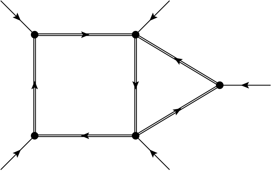
The integral corresponding to the term is the usual Feynman integral in 4 space time dimensions. It would be interesting to know if the canonical integral admits a natural interpretation in terms of Feynman integrals via integration by parts identities, or if it may be obtained from the usual Feynman integral by application of a natural differential operator in the external kinematics.
12. Example of a Stokes relation for the massive box diagram
Consider the massive pentagon diagram with arbitrary masses and external particle momenta in subject to momentum conservation. Contracting each of its edges leads to five massive box diagrams.

Since is of compact type for 1-loop graphs, we may apply corollary 10.4 to deduce a five-term relation for the massive box diagram. Indeed (10.4) implies that
| (12.1) |
where are the five diagrams pictured in figure 7. This relation can easily be checked in the massless case using Panzer’s Hyperint [Pan15].

Since the canonical integrals for massive boxes are proportional to their Feynman integrals, we deduce a 5-term relation for massive box Feynman integrals. It is known [DD98] that the latter are expressible as a linear combination of a number of dilogarithms. The graphical relation above is presumably equivalent to Abel’s 5-term equation for the dilogarithm. This functional equation should, in addition, be compatible with the motivic coaction which was computed in [Tap21].
13. Example of a canonical amplitude in the quaternionic case
13.1. A canonical amplitude for
Let be the one-loop hexagon diagram with 6 external momenta in , and 6 masses. The generalised graph Laplacian is
where is a quaternionic momentum routing. Its complex adjoint may be represented by
where we write . We find by computer calculation that
where is the determinant of the following matrix:
where we write . Thus the canonical integral associated to the massive hexagon is proportional to the usual Feynman integral (viewed in 6 spacetime dimensions). Stokes’ formula applied to a massive quaternionic heptagon diagram leads to a 7-term functional equation for these integrals.
14. Tropical single-valued integration on curves
In this section, which is not required for the paper, we provide some motivation for the definition of the generalised graph Laplacian by analogy with smooth projective algebraic curves with a finite number of punctures.
14.1. Periods on smooth algebraic curves
Let be a smooth compact curve over a field , and let denote a finite set of points. Consider the Gysin (residue) sequence in Rham cohomology
and suppose that we are given an element (‘external momentum’):
which may be interpreted as a divisor of degree on with coefficients in supported on . By pulling back the above sequence along the copy of spanned by , we obtain a simple extension over :
| (14.1) |
Since , it splits if and only if the sequence
splits. Such a splitting is given by an element (‘momentum routing’)
| (14.2) |
whose image in is . In other words, . Since , we can assume that is represented by a differential of the third kind with only logarithmic poles along . It is uniquely defined only up to adding a linear combination of holomorphic forms:
where and .
We wish to consider a Hermitian form on defined formally by:
| (14.3) | |||||
Alas, the integrals on the right are not always convergent. There are three cases:
- (1)
, and are holomorphic. Then the restiction of to is given by the convergent integrals
from which one retrieves the Riemann polarisation form. If is real, then this actually defines a symmetric quadratic form on .
- (2)
is holomorphic, and is of the third kind (or vice-versa). Then the singular integral
is convergent since it defines a single-valued period of . To see this, note that is an isomorphism and since vanishes along it may canonically be viewed as an element of . The integral above is an instance of the single-valued pairing [BD21, §6.4]:
- (3)
Only in the case does one have an ill-defined integral:
It is singular in a neighbourhood of a point , since the integrand may be expressed in local polar coordinates based at in the form
for some , which is not ‘polar-smooth’ in the terminology of [BD21]. One can regularise these integrals around each point of by a number of methods (see also [BD21, Remark 3.22]). The method used is unimportant for this discussion but the value of the integral will in general depend upon it. In any case we may simply put
where is any real and positive number of our choosing. The possibility of choosing relates to the presence of masses in Feynman graphs.
Thus, with respect to the basis of , the form is represented by a Hermitian matrix
This is precisely the form of the generalised Laplacian matrix (compare (5.4)).
14.2. Tropical analogy
Let be a connected graph (with no external half edges in the first instance). Choose an orientation on its edges. According to [MZ08], a differential form on is a linear combination
where such that for all vertices one has . Thus the space of differential forms on lies in an exact sequence
and may be identified with . The inner product on is given by
and restricts to a positive definite quadratic form on .
Now suppose that has external half-edges, and that we are given an element . As in §5.1, we deduce an extension satisfying
and the above inner product (extended -linearly) restricts to a Hermitian form
| (14.4) | |||||
which is a tropical analogue of (14.3). The generalised graph Laplacian matrix for zero masses is precisely the matrix of this Hermitian form with respect to a splitting of , which is given by any differential form
which satisfies the ‘residue’ equation for all vertices . The presence of masses corresponds, as above, to modifying only the value of in the bottom-right hand corner, and from this perspective, we see that the generalised graph Laplacian (5.4) is a tropical analogue of the regularised single-valued integration pairing discussed in §14.1.
References
- [ACP22] Daniel Allcock, Daniel Corey, and Sam Payne. Tropical moduli spaces as symmetric -complexes. Bull. Lond. Math. Soc., 54(1):193–205, 2022.
- [AHHM22] Nima Arkani-Hamed, Aaron Hillman, and Sebastian Mizera. Feynman polytopes and the tropical geometry of UV and IR divergences, 2022.
- [AHT14] Nima Arkani-Hamed and Jaroslav Trnka. The amplituhedron. Journal of High Energy Physics, 30:1029–8479, 2014.
- [BBC+20] Madeline Brandt, Juliette Bruce, Melody Chan, Margarida Melo, Gwyneth Moreland, and Corey Wolfe. On the top-weight rational cohomology of , 2020.
- [BBH20] Robert Beekveldt, Michael Borinsky, and Franz Herzog. The Hopf algebra structure of the -operation. J. High Energy Phys., 2020(7):061, 35, 2020.
- [BD21] Francis Brown and Clément Dupont. Single-valued integration and double copy. J. Reine Angew. Math., 775:145–196, 2021.
- [BEK06] Spencer Bloch, Hélène Esnault, and Dirk Kreimer. On motives associated to graph polynomials. Comm. Math. Phys., 267(1):181–225, 2006.
- [BK10] Spencer Bloch and Dirk Kreimer. Feynman amplitudes and Landau singularities for one-loop graphs. Commun. Number Theory Phys., 4(4):709–753, 2010.
- [BK13] F. Brown and D. Kreimer. Angles, scales and parametric renormalization. Lett. Math. Phys., 103(9):933–1007, 2013.
- [BK20] Marko Berghoff and Dirk Kreimer. Graph complexes and Feynman rules. Preprint: arXiv:2008.09540, 2020.
- [BM19] Marko Berghoff and Max Mühlbauer. Moduli spaces of colored graphs. Topology and its Applications, 268:106902, Dec 2019.
- [BMV11] Silvia Brannetti, Margarida Melo, and Filippo Viviani. On the tropical Torelli map. Adv. Math., 226(3):2546–2586, 2011.
- [Bor74] Armand Borel. Stable real cohomology of arithmetic groups. Ann. Sci. École Norm. Sup. (4), 7:235–272 (1975), 1974.
- [Bro10] Francis C. S. Brown. On the periods of some Feynman integrals. Preprint: arXiv:0910.0114, 2010.
- [Bro17] Francis Brown. Feynman amplitudes, coaction principle, and cosmic Galois group. Commun. Number Theory Phys., 11(3):453–556, 2017.
- [Bro21] Francis Brown. Invariant differential forms on complexes of graphs and Feynman integrals. SIGMA Symmetry Integrability Geom. Methods Appl., 17:Paper No. 103, 54, 2021.
- [BS21] M. Borinsky and O. Schnetz. Graphical functions in even dimensions. Preprint: arXiv:2105.05015, 2021.
- [BY11] Francis Brown and Karen Yeats. Spanning forest polynomials and the transcendental weight of Feynman graphs. Comm. Math. Phys., 301(2):357–382, 2011.
- [CV86] Marc Culler and Karen Vogtmann. Moduli of graphs and automorphisms of free groups. Invent. Math., 84(1):91–119, 1986.
- [DD98] A. I. Davydychev and R. Delbourgo. A geometrical angle on Feynman integrals. J. Math. Phys., 39(9):4299–4334, 1998.
- [DR22] Arnold Dresden and R. G. D. Richardson. The twenty-eighth annual meeting of the American Mathematical Society. Bull. Amer. Math. Soc., 28(4):148–164, 1922.
- [GK16] Ömer Gürdoğan and Vladimir Kazakov. New Integrable 4D Quantum Field Theories from Strongly Deformed Planar 4 Supersymmetric Yang-Mills Theory. Phys. Rev. Lett., 117(20):201602, 2016. [Addendum: Phys.Rev.Lett. 117, 259903 (2016)].
- [Gol19] Marcel Golz. Dodgson polynomial identities. Commun. Number Theory Phys., 13(4):667–723, 2019.
- [GPS17] Marcel Golz, Erik Panzer, and Oliver Schnetz. Graphical functions in parametric space. Lett. Math. Phys., 107(6):1177–1192, 2017.
- [MZ08] Grigory Mikhalkin and Ilia Zharkov. Tropical curves, their Jacobians and theta functions. In Curves and abelian varieties, volume 465 of Contemp. Math., pages 203–230. Amer. Math. Soc., Providence, RI, 2008.
- [Pan15] Erik Panzer. Algorithms for the symbolic integration of hyperlogarithms with applications to feynman integrals. Computer Physics Communications, 188:148–166, 2015.
- [Sch10] Oliver Schnetz. Quantum periods: a census of -transcendentals. Commun. Number Theory Phys., 4(1):1–47, 2010.
- [Tap21] Matija Tapušković. Motivic Galois coaction and one-loop Feynman graphs. Commun. Number Theory Phys., 15(2):221–278, 2021.
- [Tig99] Jean-Pierre Tignol. Pfaffiens et déterminant de E. H. Moore. Bull. Belg. Math. Soc. Simon Stevin, 6(4):537–539, 1999.
- [Zam80] A. B. Zamolodchikov. ‘Fishnet’ diagrams as a completely integrable system. Phys. Lett. B, 97:63–66, 1980.
- [Zha97] Fuzhen Zhang. Quaternions and matrices of quaternions. Linear Algebra Appl., 251:21–57, 1997.