A Linear Algebraic Framework
for Quantum Internet Dynamic Scheduling
Abstract
Future quantum internet aims to enable quantum communication between arbitrary pairs of distant nodes through the sharing of end-to-end entanglement, a universal resource for many quantum applications. As in classical networks, quantum networks also have to resolve problems related to routing and satisfaction of service at a sufficient rate. We deal here with the problem of scheduling when multiple commodities must be served through a quantum network based on first generation quantum repeaters, or quantum switches. To this end, we introduce a novel discrete-time algebraic model for arbitrary network topology, including transmission and memory losses, and adapted to dynamic scheduling decisions.
Our algebraic model allows the scheduler to use the storage of temporary intermediate links to optimize the performance, depending on the information availability, ranging from full global information for a centralized scheduler to partial local information for a distributed one. As an illustrative example, we compare a simple greedy scheduling policy with several Max-Weight inspired scheduling policies and illustrate the resulting achievable rate regions for two competing pairs of clients through a network.
I Introduction
Designing the Quantum Internet raises many challenges to network scientists and quantum physicists alike. Among them, the one of designing a scheduling policy is particularly familiar to the former: whenever multiple users wish to communicate through a classical network, a scheduling policy regulates fair and efficient relay of the data packets inside queues across the network routes. In the context of networks based on first generation quantum repeaters[1] or quantum switches[2, 3], users are linked through quantum entanglement swapping: letting and be two links that share one entangled pair each, entanglement swapping allows to teleport their entanglement to the link through a local measurement at node . This consumes the and pairs and yields one pair. Entangled pairs of qubits, or ebits, are a universal resource for quantum communication [4]: together with classical communications, they allow to implement a wide array of quantum protocols[5]. The task of a quantum network is therefore to distribute entanglement to multiple user pairs through a graph of interconnected quantum repeaters. Since the routes of service might not be disjoint, distribution along routes that share a subpath creates conflict that must be carefully mediated by the scheduler. In practice, a quantum scheduler must determine which swapping operations to perform at a given time, balancing between serving user requests and keeping a margin to improve future performance. Notice how the scheduling challenge naturally descends from the introduction of memories: without them, large scale networks only have the option to either swap pairs as soon as they are distributed or waste them. This work actively exploits the memory in the scheduling process, which yields the possibility for the network control system to store some pairs to swap at a following time, leveraging this additional degree of freedom through carefully taken scheduling decisions in a similar way to what [6] shows for routing. Throughout this work, the routing in the network is assumed to be fixed and known, i.e., every user pair comes with a set of routes along which the network will distribute entanglement to serve requests. We propose a linear algebraic discrete time model for quantum scheduling including all the previously mentioned factors which is suitable for any network topology including heterogeneous ones, and is dynamically controlled, i.e., the scheduling decisions are taken in real time given some degree of information on the current network state. The algebraic model is presented and formalized, and then applied to different scheduling policies: a greedy one where each node swaps randomly as soon as there is pair availability, a Max Weight[7] inspired one that has full information about the state of the network at any time and can therefore provide a best case scenario, and an intermediate one where each node solves its own individual Max Weight problem, using only local information. The achievable rate regions of these policies are shown and compared. The provided comparison ranges also in terms of localization: a global scheduler is implemented as a central block outside the network that receives information about the system’s state and broadcasts back a decision, while a localized one gives the nodes themselves the authority to decide. As will be analyzed in the dedicated section, varying the degree of localization of the scheduler changes the amount of time required for classical communication, indirectly affecting the achievable performance of the scheduler. The rest of this work has the following organization: Section II reviews the scientific context around this work, Section III describes in detail the system we are modeling and Section IV shows application of the algebraic model to real scheduling policies. Section V shows the numerical results we obtained through our model, and Section VI concludes the paper.
II Context and relevance of this work
A large amount of work in the quantum internet field consists in adapting classical network theory concepts through novel ideas that bridge the gap. An introduction to the subject and definition of the quantum network stack can be found in [8]. Delving deeper, one may see this work as an extension of [9], which treats the problem of routing without scheduling: this work deals with scheduling and adds a treatment of memory and loss. In [3, 2], a full stochastic analysis of a single quantum switch is provided and some scheduling policies are implemented on it: we state a similar problem but on an arbitrary network topology, deriving results that should prove relevant on several network scales. [10] examines the application of a Max Weight policy to quantum networks, akin to the last section of this work, the difference being that our effort focuses on the general scheduling model, with the Max Weight policy being provided as an example of its applicability. Finally, an optimal theoretical bound for entanglement distribution across a network with a single commodity is derived in [11] and expanded upon in [12]. Our work extends the treatment to multiple commodities on any arbitrary topology accounting for degrees of freedom such as memory, ebit generation statistics, technology imperfections (e.g., memory and fiber losses) and scheduling policy.
An important contribution of this work is the novel application of an idea similar to [6, 12], in a non-trivial way to general topologies and multiple commodities: the introduction of memory at the nodes allows them to decide between employing entangled pairs for swapping or keeping them for future use. The deeper implication of this point is that the network is free to create intermediate links and store them: this leads to distributing pairs across a service route in a “growing” fashion, that both increases performance and removes the need for end-to-end link state information.
III System Description
We use the following notation convention: lower case for scalars (), bold lower case for vectors (), bold upper case for matrices () and calligraphic upper case for sets (). Well-known matrices such as the identity matrix or the null matrix are indicated in blackboard bold and subscripted with their dimension (, ).
The physical system that will be modeled is a network of quantum switches. These are devices that can hold qubits and perform entanglement swapping across multiple pairs of clients, akin to a quantum repeater with multiple possible linking paths. Given an arbitrary connected graph , the switches are deployed at the locations specified by the vertices of and interconnected by lossy fiber links running along each edge . Every switch has a number of memory slots, assumed to be infinite in this work, in which qubits may be stored. Ebits (pairs of entangled qubits) are generated by each fiber link with a given constant average rate, which may be different for each link, and stored inside memories at the end nodes of the respective link. Among the network nodes, there are fixed pairs that request ebits in a random way to realize a generic application. The pairs are connected by fixed known routes that are not necessarily disjoint and therefore can create congestion across some of the network links, that needs to be managed by a scheduler. The task of the network is to distribute ebits to serve demands through entanglement swapping, while being hindered by loss: other than the losses across the fiber links, an additional form of loss is tied to memory imperfections, which cause stored qubits to effectively disappear and entanglement to be lost. Memory and fiber losses are the only two sources of imperfection that are accounted for in this paper: swaps in the switches are assumed to always succeed and memory slots at each switch are infinite, but neither of these assumptions is too limiting and they could easily be lifted in following research. For simplicity reasons, we neglect sources of state degradation other than losses in this introduction of our algebraic model, since they require a more detailed description of the quantum state of the ebits, and lead to more complex multiobjective routing and scheduling algorithms [13, 14]. Note also that our model also applies directly to more long-term quantum networks, where the ebits are logical error-corrected ebits.
For practical reasons, our model assumes a discrete time: swapping operations are supposed to occur at fixed time intervals, thus it is natural to take a discrete time step as the time unit of interest. Between two subsequent clock ticks, the system is free to evolve, and at the end of each time step a scheduling decision is taken. This places a lower bound on : no decision can happen before all information has been successfully communicated to all deciding agents, thus must be at least as large as the classical communication delay introduced by state-related information exchange. This in turn introduces a tradeoff: large means that information can travel farther before the scheduling decision is taken (allowing for larger networks or scheduling policies that require several physically spaced nodes to communicate), but it increases losses, as detailed below, and it introduces the issue of stale information: during the time it takes for state information to reach its recipient, the system continues its stochastic evolution, making the communicated data less relevant by the time it reaches the place where the scheduling decision is taken. To model ebits stored at memory nodes, the concept of an ebit queue is introduced: each pair of nodes inside the extended edge set is said to possess an ebit queue . Furthermore, among ebit queues, every associated to an edge equipped with fiber is called a physical queue, while all other ebit queues are called virtual queues. Ebit queues are an abstraction for memory slots on pairs of nodes: generation, loss and swapping may be modeled as addition, subtraction and exchange along the relevant queues. At each time step, every fiber link — and thus every physical queue — generates a number of ebits . This can model different ebit generation processes: either the physical link corresponds to a twin photon source which propagates to the switches or , or alternatively it corresponds to two photons — each one entangled with one of the switches — that meet in the middle of the link where they are subjected to a Bell state measurement (BSM). It can also model more elaborate entanglement distillation protocols or error correction based protocols based on logical qubits. Since most of these processes are probabilistic in nature will here be treated as a random process, which we assume to be Poissonian of mean value , constant in time. This allows to model the link imperfections — finite brightness of the source, propagation losses, finite success probability of photonic BSMs, etc. — as a Poisson filtration process, which simply decreases the value of . Note that need not be Poissonian: more elaborate models for are possible, e.g. to model an almost perfect pulsed periodic twin-photon source. The modelization of memory loss is slightly more complex: a qubit stored inside a quantum memory has a probability to survive for a time that is exponentially decreasing as , where is the expected lifetime of a qubit in the memory, a technological parameter expected to vary between nanoseconds and milliseconds in near term implementations [15]. By setting to the duration of a time step, we obtain the probability for a stored ebit to survive for one time step. The number of timesteps an ebit survives in memory is then given by the geometric distribution defined by . It is easy to show its mean value tends to the expected for small , being the actual lifetime of the memories. The remaining difference is an effect of the dicretization. Looking now at all the ebits in queue collectively from one timestep to the next, their losses are modeled by a binomially distributed random variable , with as many trials as there are ebits stored in queue and probability to lose one pair . Accounting for losses in such a time-dependent way makes the presented framework valid also as a tool to determine the optimal frequency at which scheduling decision should be taken, given the technological parameters.
For what concerns scheduling decisions, let indicate the number of swapping operations that happen at a given time step, at node , from queues and to queue : as a notation example, indicates three swapping operations at node from queues , to at time step . Every node will be associated to as many variables as there are swapping operations that can be performed at the node in the given routing, and the scheduler’s task will be to set such variables to control the network’s behavior. To clarify, suppose to have the service route across the users and , as shown in Fig. 1. Assume the average arrival rates to be , and . Lastly, assume that all the memories in the system have storage-and-retrieval efficiency. Fig. 2 shows the same test run but focusing on queue , to highlight the timing of the simulation.
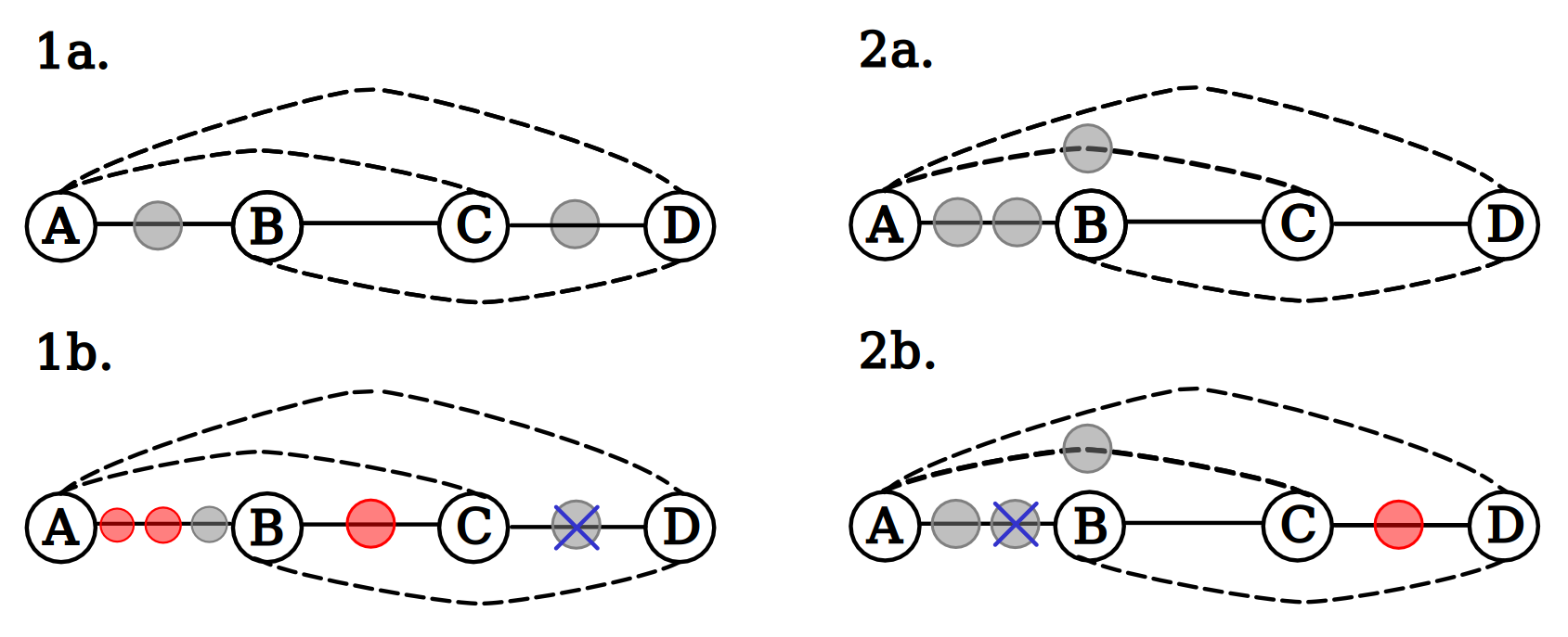

During time step 0:
- 1.
At the beginning of the time step, the queue states are: ,
- 2.
At the end of the time step, new ebits have been generated (, ) and one has been lost (). The scheduling decision is taken from this configuration as : one swap at node from queues and to .
During time step 1:
- 1.
The initial configuration sees two stored pairs in which were not employed in the last time step () and the freshly swapped one in ().
- 2.
Throughout the time step, one pair was lost across () and one generated across . The scheduler may now decide to move to or store the pairs for future use.
In term of ebits, a given transition is incoming for queue and outgoing for queues and . A queue’s evolution can therefore be summarized as follows, i.t. being a shorthand for incoming transitions, o.t. for outgoing transitions:
| (1) |
It should be noted that, while all terms of (1) are calculated for every queue, across a virtual queue will always be zero, because virtual queues do not generate ebits. Conversely, it should be stressed that the loss term is calculated in the same way for all queues, because ebit storage is always handled by memories at the network nodes: the physical/virtual queue is a mere modeling artifact to keep track of which memories store the two parts of a given ebit. A description of the whole system requires equations like (1). To keep things compact, it is useful to define some vector terms. The first ones are , and , whose entries correspond to the individual , and values (the ordering is irrelevant as long as it is consistent). Furthermore, since the effect of swapping on the queues is linear, it is possible to describe it by introducing the vector , which has elements — as many as there are allowed transitions — and a matrix with rows and columns. The vector stores all the terms, and embodies the scheduling decision, while the matrix introduces an efficient encoding of the network topology and the service routes: For each of its columns, associated to transition , the matrix has on the rows associated to queues and , and on the row associated to queue . All other terms are zero. System-wide queue evolution can be restated as the following simple linear equation:
| (2) |
Notice that eq. (2) entails an implicit assumption that the be not only a scheduling decision, but a feasible scheduling decision, i.e., one that does not cause the queues to turn negative. The meaning of this assumption will be clear when discussing partially informed scheduling policies. An example of the matrix is given in table I.
The sum of each column of is : this work only employs binary swaps, and each binary swap consumes two ebits and produces one, balancing to an overall on the total ebit count. Given a set of service routes, the matrix can be automatically generated with the code provided in the application section. The final piece of the puzzle for ebit queues is consumption: whenever there is availability of entangled pairs across one of the final pairs, the scheduler must be able to use the available pairs to serve requests. This is implemented in the model by extending the matrix to a new , and the vector to have components. What this extension achieves is to have a set of transitions that only remove one pair from a given queue, modeling actual consumption of the distributed pair by the users. Due to its construction, the matrix gives an efficient and concise description of the network topology and how the clients are connected to each other: it is therefore topology and service dependent, and provides all information about both. Putting it all together, the vector of ebit queues evolves as:
| (3) |
where the feasibility assumption from above is still taken. The introduction of consumption completes modeling of the ebits part of the system. However, there is no representation of user requests yet: in a real quantum network, users would request a given number of ebits to cater to a specific application at random times, and a well designed scheduler needs to take user requests into account when controlling the swapping network. Similarly to ebits, demands arriving to the system and being held for future service are also modeled through queues: alongside every ebit queue, there exists a demand queue that keeps track of the number of user-issued requests (as introduced in [2] for a single switch and generalized in this work for an arbitrary topology).
At each time step, every demand queue receives demands, which for simplicity are modeled as a Poisson process with average value (as in the case of ebit generation, more complex models that accurately simulate real user demands may be implemented). To maintain the model’s uniformity, all edges belonging to have a demand queue, but only the ones that are associated to an pair have nonzero arrivals. All demand queues that are not associated to an pair are permanently zero.
Demand queues have a simpler evolution than ebit ones because demands can only be generated, stored and eventually served: they are neither lost nor swapped. To model consumption without swapping, we introduce the matrix as a mean of interfacing with the consumption part of the vector. The evolution of demand queues is therefore:
| (4) |
Notice that the last components of the vector regulate both demand and ebit consumption: one demand always consumes one ebit.
IV Scheduling Application
The algebraic framework presented above poses as a tool to gauge the performance and requirements of different scheduling policies. In particular, a key point when discussing scheduling policies is the availability of information: a scheduler working with more information will understandably have much better performance but pose harsher requirements on the classical communication infrastructure that accompanies the quantum system. This creates a clear tradeoff between information requirements and performance, and the remainder of this work is dedicated to exploring it, with the ideal result being a scheduler that performs well while needing as little information as possible and with a preference for decentralized policies because they scale better.
We start by presenting a greedy scheduler which utilises minimal strictly local information: the greedy scheduler performs swapping whenever there is availability of ebits and without adapting to user demand. Therefore, in a greedy scenario, every node randomly links pairs of queues connected to it, until ebit resources are exhausted. In spite of the scheduling being random, the greedy scheduler is still aware of routing: on a linear topology with service routes and , none of the schedulers examined in this work will create entanglement because it is outside the service routes. Despite its performance being much lower than more refined schedulers, the greedy scheduler has the advantage of not requiring any information about the system’s state, thus lifting all the classical communication requirements and being completely decentralized. Its main use is as a baseline benchmark, in that any other scheduler must outperform it by a large enough margin to justify the requirement for additional information and/or communication infrastructures.
To gauge the improvement brought by additional information, we also propose an analysis of two Max Weight policies. The Max Weight protocol is a well-known result of network theory [7] [10] that revolves around solving a linear program at each time step. As soon as a queue (either ebit or demand) grows, the Max Weight scheduler will try to reduce it; the aim is to guarantee a service tailored to user requests on the demand queue side, and also efficient and fair resource exploitation on the ebit queues side, that does not lead to useless accumulation.
To fully explore the range of improvement that information availability can supply, we start from an ideal case of fully informed Max Weight scheduler: at each time step, the scheduler knows the full state of the network (…) and can therefore take the best possible decision. The discrete linear problem is stated as:
|
with the weights given by
| (8) |
where is a tunable parameter that allows to prioritize demand queues or ebit queues in the scheduling calculations. The set of all possible scheduling decisions at time slot is defined as:
| (9) | |||||
with a shorthand for the dimension of . Note that the scheduling decisions are vectors of natural numbers, each decision consuming some number of ebits.
This full knowledge scenario provides a good performance upper bound for Max Weight schedulers and a large performance margin over the greedy policy, as shown in the numerical evaluation section. Such a fully informed global scheduler is in practice unrealistic as it requires complete information about the instantaneous system state, right before each scheduling decision. In fact, the full information would require a large classical communication delay , so the scheduler would be based on stale information. This motivates to propose a scheduling policy that requires less information, while retaining to a certain level the performance benefits seen in the global-MW case. The policy should rely on a limited amount of exact quantities in the system’s state, together with suitable assumptions about unknown information in order to carry out a scheduling decision that is close to the optimal one. In particular, we propose a Max Weight inspired scheduling policy that works in a partially localized way: given a network, we assume that all nodes have access to the network’s topology, through knowledge over the matrix and know average quantities of interest, such as the intensity of Poisson generation processes , the memory efficiency and the average demand arrival rates . We furthermore assume that every node knows the exact state of the network at the beginning of each time step, i.e., and . Despite and being global information, we remind the reader that in our model this information is exact for the beginning of the time step, and is communicated during the time step , to reach all nodes by the end of the slot, when the scheduling decision is made. Moreover, each node has complete information at the end of the slot about all the queues (both physical and virtual) that are directly connected to it. This last piece of information is also available to the greedy scheduler and works as a leverage point that provides great performance improvements.
Each node states its own Max Weight problem for the whole network, combining its own perfect local information with stale information received and with expected values for the other nodes. Denoting as the set of all edges that are connected to node , the information available on node at step is
By definition , and , so the vectors of all mean arrivals are and respectively. The vectors communicated to node as well as the mean vectors are all of size . Moreover, since is the memory efficiency, .
The linear discrete scheduling problem localised on node can be stated as:
|
where the weights are given by
| (14) | |||||
Where serves the same purpose as before. The set of all possible scheduling decisions at time slot localised at node is defined as:
| (15) | |||||


After every node has solved its individual problem, all the partial solutions must be blended together to create the global solution: notice that a solution that is locally feasible may not be globally so when blended with others. To solve this issue, the notion of rank of a queue is introduced: if a queue is physical, its rank is zero. Otherwise, the rank of a queue is given by the minimum number of swapping operations required to add an ebit to it starting from an empty network. Requests are then given a random timeout, to mimic FCFS service in a real experimental system: if queues and are empty, then means a measurement is performed and fails. This failure affects the supply any hypothetical or transitions were scheduled to rely on, making them fail as well. On the other hand, correcting a decision for an outgoing transition for queues of rank has no effect on the supply for transitions from queues of rank . Therefore, both in a real system and in our model, the users’ requests are served with a FCFS discipline, in ascending rank order. The consumption part of must be handled with care too: since there is one term per queue and each queue is linked to two nodes, there are two possible candidates for each term. To keep a conservative approach, we take the minimum of the two candidates for each term. Notice that this is simply a design choice: other implementations could opt to take the maximum or design more complex schemes. If a conflict between a consumption operation and an intermediate scheduling operation arises, priority is always given to user service. We observe a great improvement in performance by this policy compared to the greedy scheduler. Moreover, as this policy is partially localized, it is practically implementable.
V Numerical Results
This section shows a numerical comparison among the presented scheduling policies through our algebraic model. All the results were obtained through a Python simulator that generates the matrix given the Alice-Bob pairs and service routes, and evaluates different policies. Its source code is available at [16]. All simulations were carried out on the topology with and as service routes, to create a bottleneck and gauge how the different schedulers handle it. One of the standard performance metrics in classical network theory is the capacity region, that can be described as follows: taking average demand from the competing clients as a set of axes, the capacity region is defined as the locus of points that the network can serve in a stable way, i.e., with all the queues returning to zero in a finite time. For our finite time simulation, we approximate the rate region by the percentage of unserved ebit requests (for an average user-demand), measured at the end of the simulation . In Fig. 3 all points in the dark blue region are certainly servable and all yellow ones are unservable, with the midway region providing an estimate for the capacity region’s bound. We opt for such a performance metric (instead of the more common average queue size) for illustration purposes, since it provides us with a sharper boundary in approximating the capacity region. All simulations were carried out on one node of the LIP6 small cluster ( x Intel Xeon E5645 cores, threads at GHz), with time steps of each and an average ebit lifetime of , yielding . was set at MHz for all links. In both the fully informed and partially informed schedulers, the weight of demands in the scheduling calculation was set to . The greedy, full information and local information schedulers took respectively half an hour, hours and hours to complete their run.
Concerning the shape of the regions reported in fig. 3, we remark that the ideal shape for a rate region in this context would be the triangle, meaning that all pairs coming to the bottleneck are effectively employed in demand service. The Full Information scheduler provides an upper bound for the potential benefits of applying Max Weight scheduling to quantum networks, while the Partial Information scheduler showcases tangible improvement with a policy that is localized enough to be reasonably implementable.
VI Conclusions and Future Perspectives
We have presented a novel algebraic model for scheduling in quantum networks and shown how it can be used to design original scheduling policies for arbitrary quantum network systems; these policies may be global or more localized for practicality. Aside from the simple Max-Weight policies here, other scheduling policies can be proposed and tested within our framework. Since the presented model takes static routes as inputs, an interesting extension to this work could be to integrate dynamic routing algorithms such as [9, 14] to obtain a full-fledged modeling toolbox to design quantum networks.
Acknowledgements
We thank Kaushik Chakraborty for stimulating discussions. PF’s work is funded by the French state through the Programme d’Investissements d’Avenir managed by the Agence Nationale de la Recherche (project ANR-21-CMAQ-0001)
References
- [1] S. Muralidharan, L. Li, J. Kim, N. Lütkenhaus, M. D. Lukin, and L. Jiang, “Optimal architectures for long distance quantum communication,” Scientific Reports, vol. 6, no. 1, p. 20463, Feb 2016. [Online]. Available: https://doi.org/10.1038/srep20463
- [2] W. Dai, A. Rinaldi, and D. Towsley, “Entanglement swapping in quantum switches: Protocol design and stability analysis,” 2021. [Online]. Available: https://arxiv.org/abs/2110.04116
- [3] G. Vardoyan, S. Guha, P. Nain, and D. Towsley, “On the stochastic analysis of a quantum entanglement distribution switch,” IEEE Transactions on Quantum Engineering, vol. 2, pp. 1–16, 2021.
- [4] M. M. Wilde, Quantum Information Theory. Cambridge university press, 2017.
- [5] “Quantum protocol zoo.” [Online]. Available: https://wiki.veriqloud.fr
- [6] E. Schoute, L. Mancinska, T. Islam, I. Kerenidis, and S. Wehner, “Shortcuts to quantum network routing,” 2016. [Online]. Available: https://arxiv.org/abs/1610.05238
- [7] L. Tassiulas and A. Ephremides, “Stability properties of constrained queueing systems and scheduling policies for maximum throughput in multihop radio networks,” IEEE Transactions on Automatic Control, vol. 37, no. 12, pp. 1936–1948, 1992.
- [8] A. Dahlberg, M. Skrzypczyk, T. Coopmans, L. Wubben, F. Rozpȩdek, M. Pompili, A. Stolk, P. Pawełczak, R. Knegjens, J. de Oliveira Filho, R. Hanson, and S. Wehner, “A link layer protocol for quantum networks,” in Proceedings of the ACM Special Interest Group on Data Communication, ser. SIGCOMM ’19. New York, NY, USA: Association for Computing Machinery, 2019, p. 159–173. [Online]. Available: https://doi.org/10.1145/3341302.3342070
- [9] M. Pant, H. Krovi, D. Towsley, L. Tassiulas, L. Jiang, P. Basu, D. Englund, and S. Guha, “Routing entanglement in the quantum internet,” npj Quantum Information, vol. 5, no. 1, p. 25, Mar 2019. [Online]. Available: https://doi.org/10.1038/s41534-019-0139-x
- [10] T. Vasantam and D. Towsley, “Stability analysis of a quantum network with max-weight scheduling,” 2021. [Online]. Available: https://arxiv.org/abs/2106.00831
- [11] W. Dai, T. Peng, and M. Z. Win, “Optimal remote entanglement distribution,” IEEE Journal on Selected Areas in Communications, vol. 38, no. 3, pp. 540–556, 2020.
- [12] W. Dai and D. Towsley, “Entanglement swapping for repeater chains with finite memory sizes,” 2021. [Online]. Available: https://arxiv.org/abs/2111.10994
- [13] L. Bugalho, B. C. Coutinho, F. A. Monteiro, and Y. Omar, “Distributing multipartite entanglement over noisy quantum networks,” 2021. [Online]. Available: https://arxiv.org/abs/2103.14759
- [14] K. Chakraborty, D. Elkouss, B. Rijsman, and S. Wehner, “Entanglement distribution in a quantum network: A multicommodity flow-based approach,” IEEE Transactions on Quantum Engineering, vol. 1, pp. 1–21, 2020.
- [15] M. Cao, F. Hoffet, S. Qiu, A. S. Sheremet, and J. Laurat, “Efficient reversible entanglement transfer between light and quantum memories,” Optica, vol. 7, no. 10, p. 1440, oct 2020. [Online]. Available: https://doi.org/10.1364%2Foptica.400695
- [16] “Simulator github repository.” [Online]. Available: https://github.com/pfittipaldi/DynSchedSimulator