BayesPCN: A Continually Learnable
Predictive Coding Associative Memory
Abstract
Associative memory plays an important role in human intelligence and its mechanisms have been linked to attention in machine learning. While the machine learning community’s interest in associative memories has recently been rekindled, most work has focused on memory recall () over memory learning (). In this paper, we present BayesPCN, a hierarchical associative memory capable of performing continual one-shot memory writes without meta-learning. Moreover, BayesPCN is able to gradually forget past observations () to free its memory. Experiments show that BayesPCN can recall corrupted i.i.d. high-dimensional data observed hundreds to a thousand “timesteps” ago without a large drop in recall ability compared to the state-of-the-art offline-learned parametric memory models.
1 Introduction
One of the hallmarks of biological intelligence is the ability to robustly recall learned associations. Biological agents are able to associate stimuli of various modalities and rely on their memories to perform everyday tasks from navigation to entity recognition. Yet these agents are not only good at recall but can quickly and continually form new memories from as little as a single experience. How do biological agents achieve this feat while mitigating catastrophic forgetting (French 1999)? And how can we build neural networks that demonstrate these properties? This paper addresses these questions, focusing on fast, continual learning of neural artifacts that perform robust recall of i.i.d. high-dimensional observations.
Associative memory models have been of interest in machine learning for decades (Steinbuch 1961; Hopfield 1982). They have been used to solve a wide range of problems from sequence processing (Schmidhuber 1992; Graves et al. 2014; Schlag et al. 2021) to pattern detection (Widrich et al. 2020; Widrich et al. 2021; Seidl et al. 2021). Their study has allowed us to build models that replicate aspects of biological intelligence (Kanerva 1988; Hawkins and Blakeslee 2004) and provided novel perspectives on machine learning toolsets like dot-product attention, transformers, and linear layers of deep neural networks (Ramsauer et al. 2020; Bricken and Pehlevan 2021; Irie et al. 2022).
Our main aim is to recall exact memories from a neural network that can rapidly and continually learn from a stream of data. Towards this end we introduce BayesPCN, a Bayesian take on the generative predictive coding network (GPCN) (Salvatori et al. 2021) that combines predictive coding and locally conjugate Bayesian updates11 1 Code is available at https://github.com/plai-group/bayes-pcn. There are currently a number of associative memory systems that are continually learnable (Hopfield 1982; Kanerva 1988; Hawkins and George 2007; Ramsauer et al. 2020; Sharma et al. 2022). However, to our knowledge, BayesPCN is the first parametric associative memory model to continually learn hundreds of high-dimensional observations while maintaining good recall performance on inputs with nontrivial amounts of corruption. In addition, it is also the first hierarchical memory which after repeated forgetting recovers its original memory state.
2 Background
2.1 Auto-Associative and Hetero-Associative Memory
Before we begin let us review two useful concepts: auto-associative memory and hetero-associative memory. The former, auto-associative memory, refers to a memory system that is content addressable but for which the query may be a corrupted version of the original data item. One can think about auto-associative memory systems as a kind of approximate nearest neighbor lookup mechanism. Hetero-associative memory systems are key-value stores, meaning that the recalled “value” is potentially of a different type to the “key.” Crucially, hetero-associative memory systems can, in large part, be implemented by auto-associative memory systems by forming a “joint” object to memorize by combining the key and value into one object. Hetero-associative queries can then be processed simply by looking up the joint object “corrupted” by discarding the value.
2.2 Generative Predictive Coding Network
A generative predictive coding network (GPCN) (Salvatori et al. 2021) is an energy-based associative memory model that has set the state-of-the-art on a number of image associative recall tasks. As illustrated in Figure 2, GPCN takes the form of a fully connected neural network whose bottom layer activations characterize the sensory inputs and higher layer activations characterize the internal representations of the sensory inputs. GPCN’s operation (recall) initializes the bottom layer activations to the input query vector and iteratively denoises the query until a stored value is retrieved by minimizing its energy function w.r.t. some or all of its neuron activations. GPCN’s operation (learning) adapts the network parameters to shape the energy function such that the stored datapoints become the local minima of the energy function.
Before describing GPCN’s and mechanisms in more detail, we introduce the notation we use in this paper. Let be a GPCN with layers of neurons where and denotes the bottom and the top layer index respectively. Then, let be the width of the -th layer, be the row vector denoting the -th layer’s pre-activation function neuron values, and be the -th layer’s activation function, for instance ReLU. In addition, let where be the synaptic weight matrix between +-th and -th layers and be the “bias” row vector that influences the dynamics of the top layer neuron activities . One can intuitively think of the model parameters as the memory content and the activations as the read state of the memory.
GPCN’s and are facilitated by predictive coding (PC) (Rao and Ballard 1999), a biologically plausible learning rule that can approximate backpropagation (Millidge et al. 2020). PC’s energy function is the sum of prediction errors across all network layers. For GPCN, the choice of prediction error is the squared Euclidean distance between the actual layer activations and the prediction of the same layer activations made by their immediate upper layer activations. This leads to the following energy function.
| (1) |
GPCN’s performs gradient descent on the energy w.r.t. some or all of after setting the initial values of to the memory query and fixing the values of . GPCN’s obtains the output for each of i.i.d. datapoints to store , takes a gradient step on the energy w.r.t. while fixing , and repeats until convergence.
We now take a probabilistic perspective on GPCN. One can view GPCN as a hierarchical generative model where all neuron activations are modeled by normally distributed random variables and the link function between the subsequent layers is a layer-specific nonlinearity followed by a linear transform. Then, GPCN’s - the minimization of Equation 1 - is equivalent to maximizing the log density in Equation 2 w.r.t. .
| (2) |
In other words, GPCN’s performs iterated conditional modes (Besag 1986) on the hierarchical generative model in the neuron activation space (refer to Algorithms 3 and 4). In addition, GPCN’s can be viewed as an approximate maximization of the lower bound on w.r.t. (Millidge et al. 2021). This follows from the fact that GPCN learns via PC.
While GPCN possesses impressive associative recall capabilities, the learning rule proposed in Salvatori et al. 2021 is not amenable to continual learning. Due to its lack of safeguards against catastrophic forgetting, continually learning GPCN leads to a forgetting of information associated with older observations or requires a costly offline model refitting on all observations whenever a new datapoint is observed. BayesPCN’s foremost aim is to address this limitation while preserving GPCN’s capabilities as much as possible.
3 Memory Model
BayesPCN is structurally identical to GPCN, but unlike GPCN the network parameters are treated as latent random variables. This allows BayesPCN’s operation to be cast as (approximate) posterior inference over given new observations in a way similar to (Wu et al. 2018a). In other words, storing i.i.d. datapoints into memory is equivalent to estimating . Figure 2 illustrates the graphical model for BayesPCN.
We now review the probabilistic structure of BayesPCN. We assume that, prior to any observations, the random variables (where is the datapoint index) are distributed as follows
| (3) | ||||
| (4) |
where and denotes normal and matrix normal distribution (Gupta and Nagar 2018) respectively. We remind the readers that the matrix normal distribution is a normal distribution for matrix-variate data that compactly specifies the matrix elements’ means, row-wise covariances, and column-wise covariances. The joint distribution over all random variables when there are sensory observations is, due to the conditional independence of given ,
| (5) |
We note that BayesPCN’s structure leads to two desirable properties that become useful when approximating during the operation. First, by exploiting the linear Gaussian marginalization formula and conditional independence we can analytically compute the marginal distribution over all activation vectors .
| (6) | ||||
| (7) |
We stress that neither nor has an analytic form due to the presence of nonlinearities. In addition, if all activation vectors are observed, the posterior over the model parameters becomes normally distributed due to the linear Gaussian posterior formula and the fact that are conditionally independent given (the analytical posterior formulae for Equation 9 are in Appendix C).
| (8) | ||||
| (9) |
We use to denote the sufficient statistics of the layer-wise network weight posterior distributions given .
4 Memory Operations
This section contains the memory operations that BayesPCN supports: , , and . We use the shorthand to denote all hidden layer neuron activations and to denote all network parameters.
4.1 Read
The operation takes the corrupted query vector and retrieves the memory’s best guess of the associated original datapoint . As in GPCN, this is done by hill climbing the memory’s log density w.r.t. the neuron activations . To clarify, is the current memory read state and is not directly related to the past observations . BayesPCN’s auto-associative recall performs iterated conditional modes on w.r.t. and BayesPCN’s hetero-associative recall performs gradient ascent on w.r.t. while keeping the known values of fixed. Algorithm 3 and Algorithm 4 in Appendix A, the recall procedures taken from Salvatori et al. 2021 and rewritten from the probabilistic perspective, describe this in more detail.
4.2 Write
The operations aims to take the previous timestep posterior over the model parameters and the current timestep observation to return the current timestep posterior over the model parameters . Unfortunately, the analytical form of is unavailable due to the presence of nonlinearities in BayesPCN so one must resort to approximate posterior inference.
We propose a sequential importance sampling posterior inference algorithm for estimating where the particles are high-dimensional Gaussian distributions. Let be the number of sequential importance sampling particles and be the particle index. The -th timestep posterior estimate is recursively represented as a weighted Gaussian mixture of the form where is the -th particle’s importance weight and is the -th particle’s activation conditioned posterior described in Equation 8. We note that each is efficiently characterised by the sufficient statistics . Algorithm 1 describes the operation in detail (see Appendix B for its justification).
While in principle can be any distribution, BayesPCN’s sets it to as is standard in predictive coding (Millidge et al. 2021). In addition, we define the BayesPCN parameter prior (of an “empty” memory) as where are initialized using Kaiming initialization. We chose this prior over a non-mixture prior to obtain a multi-particle posterior approximation despite using a Dirac variational distribution.
We now direct our attention to obtaining used in the operations from . Using Equation 6, we obtain the approximate posterior predictive density
| (10) | ||||
| (11) |
BayesPCN’s can be seen as a special case of sequential imputation (Kong et al. 1994), an online parameter inference algorithm that represents the parameter posterior conditioned on partial observations as a mixture of parameter posteriors conditioned on complete observations. In addition, whereas the parameter update proposed by Salvatori et al. 2021 is doing local gradient descent for each , BayesPCN’s parameter update is doing local conjugate normal-normal Bayesian update for each . Hence, like GPCN, BayesPCN’s synaptic weight update only utilizes local information. Lastly, while exact Bayesian updates are invariant to the order of observations, because we are using predictive coding to fit the variational distribution BayesPCN’s is technically not invariant to the order of observations.
4.3 Forget
We also propose a diffusion-based forgetting mechanism for BayesPCN. As more datapoints are written into a BayesPCN model, the model’s belief over the true parameter location shifts and the uncertainty over its belief decreases. This has the effect of making the model’s parameters less adaptive to new datapoints and typically magnifying ’s norms as the prior’s contribution weakens. One can interpret this as the memory being overloaded. The operation counteracts this phenomenon by nudging the model’s belief over toward the prior (empty memory state) and increasing its uncertainty proportional to the forget strength parameter . Algorithm 2 describes this in detail (the analytical diffusion formulae are in Appendix D).
If applied an infinite number of times, reverts the posterior over the parameters to the prior due to the property of diffusion if the particle weights are uniform. In practice, one would apply periodically or when the memory starts to become overloaded from too much data and stops being performant. Because erases stored information for all of datapoints somewhat evenly, the datapoints from the distant past that was applied to more would be, as the name suggests, more forgotten than the recent datapoints that was applied to less.
5 Related Work
We briefly review the most relevant work to BayesPCN, starting with the predictive coding networks. As covered in Section 2, GPCN (Salvatori et al. 2021) is the model that BayesPCN is built upon. Self-taught associative memory (Dovrolis 2018; Smith et al. 2021) is a hierarchical predictive coding memory that performs unsupervised continual learning using online clustering modules as building blocks, unlike BayesPCN’s building blocks of artificial neurons. The sequential neural coding network (Ororbia et al. 2019; Ororbia et al. 2018), while not explicitly used as an associative memory, is also a continually learned predictive coding network similar in structure to GPCN that combats catastrophic forgetting via task-dependent activation sparsity. BayesPCN on the other hand combats catastrophic forgetting by incorporating uncertainty over the synaptic weights.
Moving on to general attractor-based memory models, Hopfield networks (Hopfield 1982) and their modern variants (Krotov and Hopfield 2016; Ramsauer et al. 2020; Krotov and Hopfield 2020; Krotov 2021; Millidge et al. 2022) are biologically motivated auto-associative memories that define the neuron activation dynamics via Lagrangian functions. Out of these models only Krotov 2021’s model is hierarchical, but theirs is not continually learned. BayesPCN generalizes the modern Hopfield network and fits into the universal Hopfield network’s similarity-separation-projection paradigm for associative memories (refer to Appendix E). Sparse Distributed Memory (SDM) (Kanerva 1988) is a non-hierarchical memory that exploits high-dimensionality to perform auto-associative and hetero-associative recall. Hierarchical Temporal Memory (HTM) (Hawkins and George 2007; Cui et al. 2016) is a biologically constrained hierarchical memory that continually learns time-based patterns with sparse representations. HTM does not employ predictive coding and to our knowledge has not yet been tested on high-dimensional data.
Relative to generative modeling and memory research, our work has connections to the Kanerva machine’s memory as inference approach (Wu et al. 2018a; Wu et al. 2018b) and the one-shot memory write from Bartunov et al. 2019; Pham et al. 2022. These papers’ models employ meta-learning unlike aforementioned work. We note that the Kanerva machine also applies conjugate normal-normal Bayesian update to adapt its top level memory matrix once the model is meta-learned via end-to-end gradient descent. On the other hand, BayesPCN applies conjugate normal-normal Bayesian update to all of its weight matrices and this as of itself constitutes learning.
6 Experiments
This section assesses BayesPCN’s recall capabilities on image recovery tasks and examines the effect of on BayesPCN’s behaviour.
We used CIFAR10 (Krizhevsky et al. 2009) and Tiny ImageNet (Le and Yang 2015) datasets for all experiments, whose images are of size and respectively. During the phase of the experiments, BayesPCN models were given one image to store into their memories per timestep for up to 1024 images. Then, during the phase of the experiments, we recorded the pixel-wise mean squared error (MSE) between the phase images and the models’ outputs given the corrupted phase images as inputs. For reference, the pixel-wise MSE of is distinguishable to human eyes on close inspection of the images.
BayesPCN models were compared against identity models (models that return their inputs as outputs), modern Hopfield networks (MHN) (Ramsauer et al. 2020), and vanilla GPCNs (Salvatori et al. 2021) all of which were offline learned. We note that GPCNs have set the state-of-the-art on CIFAR10 and TinyImageNet image recall tasks. BayesPCN models were also compared against online GPCNs, GPCNs that naively applied their offline memory to sequentially arriving observations and memorized one image per timestep for up to 1024 images. We used our own autodiff implementation of MHNs based on Appendix E. See Appendix F for additional experiment details.
6.1 Auto-Associative and Hetero-Associative Read
For the auto-associative recall experiments, the memory inputs at the phase were the phase images corrupted by pixel-wise white noise with standard deviation . For the hetero-associative recall experiments, we tested two types of training image corruption schemes. The first type, dropout, randomly blacked out 25% of the image pixels. The second type, mask, blacked out 25% of the rightmost image pixels. Image recovery under these settings is hetero-associative recall because one can view the non-blacked out pixels as the “key” and the blacked out pixels as the “value”. We experimented with 4-layer BayesPCN models that have hidden layer sizes of 256, 512, and 1024, particle counts of 1 and 4, and activation functions ReLU and GELU. We searched over the same hyperparameters for offline and online 4-layer GPCNs aside from the particle count. Lastly, we evaluated 4-layer BayesPCN models, which we denote as BayesPCN (), that applied with strength to their weights once every 64 operations.
| White Noise CIFAR10 MSE | ||||
| Sequence Length | 128 | 256 | 512 | 1024 |
| Identity | 0.1596 | 0.1600 | 0.1600 | 0.1600 |
| MHN | 0.0000 | 0.0000 | 0.0000 | 0.0000 |
| GPCN (Offline) | 0.0028 | 0.0046 | 0.0073 | 0.0121 |
| GPCN (Online) | 0.0103 | 0.0150 | 0.0191 | 0.0210 |
| BayesPCN | 0.0017 | 0.0085 | 0.0146 | 0.0337 |
| BayesPCN () | 0.0064 | 0.0102 | 0.0145 | 0.0188 |
| White Noise Tiny ImageNet MSE | ||||
| Sequence Length | 128 | 256 | 512 | 1024 |
| Identity | 0.1600 | 0.1602 | 0.1601 | 0.1600 |
| MHN | 0.0000 | 0.0000 | 0.0000 | 0.0000 |
| GPCN (Offline) | 0.0005 | 0.0010 | 0.0018 | 0.0067 |
| GPCN (Online) | 0.0089 | 0.0112 | 0.0138 | 0.0181 |
| BayesPCN | 0.0011 | 0.0033 | 0.0064 | 0.6606 |
| BayesPCN () | 0.0026 | 0.0059 | 0.0108 | 0.0176 |
| Dropout CIFAR10 MSE | ||||
| Sequence Length | 128 | 256 | 512 | 1024 |
| Identity | 1.1140 | 1.1178 | 1.1353 | 1.1481 |
| MHN | 0.0000 | 0.0000 | 0.0000 | 0.0000 |
| GPCN (Offline) | 0.0000 | 0.0000 | 0.0000 | 0.0001 |
| GPCN (Online) | 0.0022 | 0.0032 | 0.0053 | 0.0073 |
| BayesPCN | 0.0000 | 0.0000 | 0.0000 | 0.0001 |
| BayesPCN () | 0.0000 | 0.0001 | 0.0005 | 0.0019 |
| Dropout Tiny ImageNet MSE | ||||
| Sequence Length | 128 | 256 | 512 | 1024 |
| Identity | 1.0629 | 1.0889 | 1.1154 | 1.1072 |
| MHN | 0.0000 | 0.0000 | 0.0000 | 0.0000 |
| GPCN (Offline) | 0.0000 | 0.0000 | 0.0000 | 0.0000 |
| GPCN (Online) | 0.0036 | 0.0053 | 0.0069 | 0.0099 |
| BayesPCN | 0.0000 | 0.0000 | 0.0000 | 0.0000 |
| BayesPCN () | 0.0000 | 0.0000 | 0.0002 | 0.0008 |
| Mask CIFAR10 MSE | ||||
| Sequence Length | 128 | 256 | 512 | 1024 |
| Identity | 1.1272 | 1.1373 | 1.1619 | 1.1653 |
| MHN | 0.0000 | 0.0000 | 0.0011 | 0.0000 |
| GPCN (Offline) | 0.0000 | 0.0000 | 0.0000 | 0.0009 |
| GPCN (Online) | 0.0127 | 0.0255 | 0.0522 | 0.0791 |
| BayesPCN | 0.0000 | 0.0000 | 0.0001 | 0.0019 |
| BayesPCN () | 0.0000 | 0.0008 | 0.0096 | 0.0465 |
| Mask Tiny ImageNet MSE | ||||
| Sequence Length | 128 | 256 | 512 | 1024 |
| Identity | 1.0876 | 1.0884 | 1.0982 | 1.1132 |
| MHN | 0.0000 | 0.0000 | 0.0000 | 0.0010 |
| GPCN (Offline) | 0.0000 | 0.0000 | 0.0000 | 0.0001 |
| GPCN (Online) | 0.0081 | 0.0316 | 0.0441 | 0.0698 |
| BayesPCN | 0.0000 | 0.0000 | 0.0000 | 0.0000 |
| BayesPCN () | 0.0000 | 0.0003 | 0.0031 | 0.0235 |
Table 1 shows the average MSE between the ground truth images and the associative memory outputs for models trained on data sequences of different lengths, where the reported scores come from the best models of each category. The results were averaged across three random seeds. Appendix I details how different hyperparameter values affect BayesPCN’s performance.
BayesPCN’s recall errors were on par with offline GPCN’s recall errors and were orders of magnitude lower than online GPCN’s recall errors on all hetero-associative recall tasks and sequence lengths. BayesPCN () performed worse than BayesPCN in these settings but still outperformed online GPCN on all hetero-associative recall tasks and sequence lengths. On auto-associative recall tasks with sequences of length , BayesPCN’s recall errors were marginally higher than offline GPCN’s recall errors but lower than online GPCN’s recall errors. However, when the sequence length approached 1024, BayesPCN performed worse than online GPCN and on the TinyImageNet auto-associative recall task became even worse than the identity model. We hypothesize that BayesPCN’s sudden performance drop stems from the fact that it is not “removing” old information unlike online GPCN and BayesPCN () due to the conjugate Bayesian update’s observation order invariance property. This causes BayesPCN to approach the overloaded memory regime, where recall of all data suffers, once enough information has been stored. Because BayesPCN () deliberately removes old information and thus is farther away from the overloaded memory regime, it was able to outperform online GPCN on all auto-associative recall tasks and sequence lengths.
GPCN and BayesPCN models overall found hetero-associative recall easier than auto-associative recall, likely because the former fixes the key bits during memory and thus discourages the algorithm from wandering to less realistic values. Counterintuitively, GPCN and BayesPCN models were better at Tiny ImageNet recall over CIFAR10 recall. We attribute this behaviour to the fact that for some models, high-dimensional data recall can ironically be easier than low-dimensional data recall because individual datapoints are further apart from one another in higher dimensions.
A surprising discovery from this experiment was how good MHN’s recall can be compared to GPCN and BayesPCN’s recall when the memory query had a moderate amount of noise, a result inconsistent with the findings from Salvatori et al. 2021. Because MHN explicitly retains past observations in a data matrix and its softmax inverse temperature was set very high (), MHN’s recall effectively selected the observation that had the highest dot-product similarity to the memory query in our experiments. In Appendix G, we assess how MHN’s recall compares to BayesPCN’s recall when the memory query corruption is much higher. As expected, because the observation with the highest dot-product similarity to the memory query is often not the right image to recall, BayesPCN significantly outperformed MHN in hetero-associative recall tasks.
6.2 Forgetting
This section investigates the operation’s effect on BayesPCN’s recall behaviour. Specifically, we show that causes BayesPCN to better recall recent observations at the expense of older observations and that this effect is more pronounced the higher the forget strength is. We trained six structurally identical BayesPCN models on 1024 CIFAR10 images sequentially and applied with strength to each model once after every 64 operations.
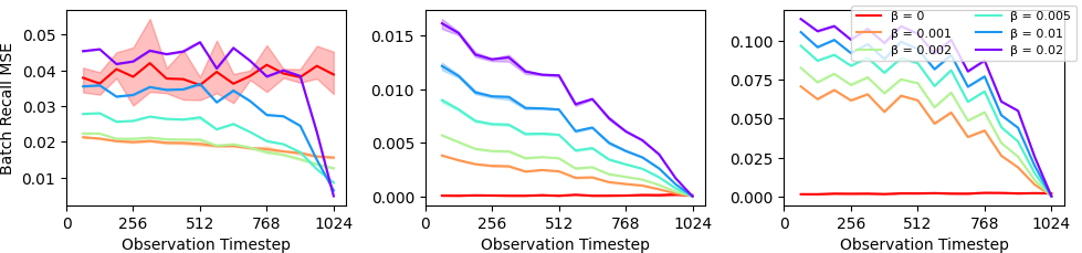
Figure 3 compares the models’ recall MSE on 16 data batches of size 64 that were observed during different points of the training once the models have observed all 1024 datapoints. We see that BayesPCN with no performs similarly on all datapoints regardless of their observation timestep, which is likely the consequence of conjugate Bayesian update’s observation order invariance. On the other hand, BayesPCNs with consistently perform better on newer datapoints with this effect being strongly correlated with the value of . As previously shown, some amount of forgetting during training can improve the overall performance of the memory across all datapoints over no forgetting for long training sequences. Lastly, the higher the forget strength was the lower the recall error on the most recent data batch was for all tasks and forget strength values.
7 Discussion
One can intuitively think of BayesPCN as an approximate nearest neighbour operation with a learned similarity metric and as the continual learning of that metric. MHN on the other hand uses the dot-product distance as its similarity metric (Millidge et al. 2022). This explains why MHN is not good at highly masked image recall because from a pixelwise dot-product distance perspective, highly masked image queries are often closer to unrelated images than to the ground truth images.
BayesPCN is closely related to the predictive coding theories of the brain’s memory system. For example, Barron et al. 2020 suggests that the hippocampus may correspond to the top layer of a predictive coding network and the neo-cortical areas may correspond to the rest of the predictive coding network. Similarly, Dovrolis 2018 posits that their predictive coding network could serve as a model of the cortical column albeit without experimental results. It is however unclear how exactly BayesPCN’s activation gradient descent and locally conjugate Bayesian weight update can be realized in the brain. Lastly, there are similarities between BayesPCN’s diffusion-based and the synaptic homeostasis hypothesis (Cirelli and Tononi 2022), where during sleep synaptic weight strengths are decreased on average to facilitate future learning.
Aside from these biological connections, BayesPCN has many potential machine learning applications. One possible line of work is using it in conjunction with a neural controller that learns what information to store into memory (Graves et al. 2014; Schlag et al. 2021). Using BayesPCN in this way would confer the benefit of high query noise tolerance for neural controllers. Another line of work is using it to solve small data supervised learning problems, leveraging the fact that nearest neighbour methods work well when data availability is sparse (Ramsauer et al. 2020).
To conclude, we introduced BayesPCN, an associative memory model that can robustly retrieve past observations given various corrupted inputs, perform one-shot parameter update of a deep neural network to store new observations as attractors, and forget old observations to better store newer ones. We demonstrated that BayesPCN’s recall performance is in most cases not significantly worse than the recall performance of its offline-learned counterpart even though it is continually learned. There are several intriguing extensions to BayesPCN that may address some of its limitations. Currently, BayesPCN can take up to thousands of activation gradient descent iterations to obtain the best recall result when a lot of data has been stored into memory. Supplementing BayesPCN with amortized inference may greatly reduce this computational requirement (Tschantz et al. 2022). In addition, BayesPCN can return a nonsensical output if the memory query is too far away from the stored datapoints or if the memory is overloaded. Investigating BayesPCN’s latent landscape may allow us design models with more robust basin of attractions that can easily be reached via activation gradient descent. Last but not least, extending BayesPCN beyond memorizing i.i.d. data to memorizing sequences like the human episodic memory would be of great interest.
Acknowledgments and Disclosure of Funding
We would like to thank Boyan Beronov for the helpful discussions. In addition, we acknowledge the support of the Natural Sciences and Engineering Research Council of Canada (NSERC), the Canada CIFAR AI Chairs Program, and the Intel Parallel Computing Centers program. Additional support was provided by UBC’s Composites Research Network (CRN), and Data Science Institute (DSI). This research was enabled in part by technical support and computational resources provided by WestGrid (www.westgrid.ca), Compute Canada (www.computecanada.ca), and Advanced Research Computing at the University of British Columbia (arc.ubc.ca).
References
- Barron et al. [2020] Helen C. Barron, Ryszard Auksztulewicz, and Karl Friston. Prediction and memory: A predictive coding account. Progress in Neurobiology, 192:101821, 2020. ISSN 0301-0082. doi: https://doi.org/10.1016/j.pneurobio.2020.101821. URL https://www.sciencedirect.com/science/article/pii/S0301008220300769.
- Bartunov et al. [2019] Sergey Bartunov, Jack W Rae, Simon Osindero, and Timothy P Lillicrap. Meta-learning deep energy-based memory models. arXiv preprint arXiv:1910.02720, 2019.
- Besag [1986] Julian Besag. On the statistical analysis of dirty pictures. Journal of the Royal Statistical Society: Series B (Methodological), 48(3):259–279, 1986.
- Bricken and Pehlevan [2021] Trenton Bricken and Cengiz Pehlevan. Attention approximates sparse distributed memory. Advances in Neural Information Processing Systems, 34, 2021.
- Cirelli and Tononi [2022] Chiara Cirelli and Giulio Tononi. The why and how of sleep-dependent synaptic down-selection. Seminars in Cell & Developmental Biology, 125:91–100, 2022. ISSN 1084-9521. doi: https://doi.org/10.1016/j.semcdb.2021.02.007. URL https://www.sciencedirect.com/science/article/pii/S1084952121000318. Special Issue: Interplay between non-canonical and canonical Wnt signalling by Terry Van Raay/ Special Issue: The making of memories by Patricio Opazo and Victor Anggono.
- Cui et al. [2016] Yuwei Cui, Subutai Ahmad, and Jeff Hawkins. Continuous online sequence learning with an unsupervised neural network model. Neural Computation, 28(11):2474–2504, nov 2016. doi: 10.1162/neco_a_00893. URL https://doi.org/10.1162%2Fneco_a_00893.
- Dovrolis [2018] Constantine Dovrolis. A neuro-inspired architecture for unsupervised continual learning based on online clustering and hierarchical predictive coding, 2018. URL https://arxiv.org/abs/1810.09391.
- French [1999] Robert M French. Catastrophic forgetting in connectionist networks. Trends in cognitive sciences, 3(4):128–135, 1999.
- Graves et al. [2014] Alex Graves, Greg Wayne, and Ivo Danihelka. Neural turing machines, 2014. URL https://arxiv.org/abs/1410.5401.
- Gupta and Nagar [2018] A.K. Gupta and D.K. Nagar. Matrix Variate Distributions. Monographs and Surveys in Pure and Applied Mathematics. CRC Press, 2018. ISBN 9781351433006. URL https://books.google.ca/books?id=Tl1ZDwAAQBAJ.
- Hawkins and Blakeslee [2004] Jeff Hawkins and Sandra Blakeslee. On Intelligence. Times Books, New York, 2004.
- Hawkins and George [2007] Jeffrey Hawkins and Dileep George. Directed behavior using a hierarchical temporal memory based system, August 16 2007. US Patent App. 11/622,448.
- Hopfield [1982] John J Hopfield. Neural networks and physical systems with emergent collective computational abilities. Proceedings of the national academy of sciences, 79(8):2554–2558, 1982.
- Irie et al. [2022] Kazuki Irie, Róbert Csordás, and Jürgen Schmidhuber. The dual form of neural networks revisited: Connecting test time predictions to training patterns via spotlights of attention. In Proceedings of the 39th International Conference on Machine Learning, volume 162 of Proceedings of Machine Learning Research, pages 9639–9659. PMLR, 17–23 Jul 2022. URL https://proceedings.mlr.press/v162/irie22a.html.
- Kanerva [1988] Pentti Kanerva. Sparse distributed memory. MIT press, 1988.
- Kong et al. [1994] Augustine Kong, Jun S Liu, and Wing Hung Wong. Sequential imputations and bayesian missing data problems. Journal of the American statistical association, 89(425):278–288, 1994.
- Krizhevsky et al. [2009] Alex Krizhevsky, Geoffrey Hinton, et al. Learning multiple layers of features from tiny images. 2009.
- Krotov [2021] Dmitry Krotov. Hierarchical associative memory. arXiv preprint arXiv:2107.06446, 2021.
- Krotov and Hopfield [2020] Dmitry Krotov and John Hopfield. Large associative memory problem in neurobiology and machine learning. arXiv preprint arXiv:2008.06996, 2020.
- Krotov and Hopfield [2016] Dmitry Krotov and John J Hopfield. Dense associative memory for pattern recognition. 2016. doi: 10.48550/ARXIV.1606.01164. URL https://arxiv.org/abs/1606.01164.
- Le and Yang [2015] Ya Le and Xuan Yang. Tiny imagenet visual recognition challenge. CS 231N, 7(7):3, 2015.
- Millidge et al. [2020] Beren Millidge, Alexander Tschantz, and Christopher L. Buckley. Predictive coding approximates backprop along arbitrary computation graphs, 2020. URL https://arxiv.org/abs/2006.04182.
- Millidge et al. [2021] Beren Millidge, Anil Seth, and Christopher L Buckley. Predictive coding: a theoretical and experimental review, 2021. URL https://arxiv.org/abs/2107.12979.
- Millidge et al. [2022] Beren Millidge, Tommaso Salvatori, Yuhang Song, Thomas Lukasiewicz, and Rafal Bogacz. Universal hopfield networks: A general framework for single-shot associative memory models. arXiv preprint arXiv:2202.04557, 2022.
- Ororbia and Kifer [2022] Alexander Ororbia and Daniel Kifer. The neural coding framework for learning generative models. Nature Communications, 13(1), April 2022. doi: 10.1038/s41467-022-29632-7. URL https://doi.org/10.1038/s41467-022-29632-7.
- Ororbia et al. [2019] Alexander Ororbia, Ankur Mali, Daniel Kifer, and C. Lee Giles. Lifelong neural predictive coding: Learning cumulatively online without forgetting, 2019. URL https://arxiv.org/abs/1905.10696.
- Ororbia et al. [2018] Alexander G. Ororbia, Ankur Mali, Daniel Kifer, and C. Lee Giles. Conducting credit assignment by aligning local representations, 2018. URL https://arxiv.org/abs/1803.01834.
- Pham et al. [2022] Kha Pham, Hung Le, Man Ngo, Truyen Tran, Bao Ho, and Svetha Venkatesh. Generative pseudo-inverse memory. In International Conference on Learning Representations, 2022. URL https://openreview.net/forum?id=Harn4_EZBw.
- Ramsauer et al. [2020] Hubert Ramsauer, Bernhard Schäfl, Johannes Lehner, Philipp Seidl, Michael Widrich, Thomas Adler, Lukas Gruber, Markus Holzleitner, Milena Pavlović, Geir Kjetil Sandve, et al. Hopfield networks is all you need. arXiv preprint arXiv:2008.02217, 2020.
- Rao and Ballard [1999] Rajesh PN Rao and Dana H Ballard. Predictive coding in the visual cortex: a functional interpretation of some extra-classical receptive-field effects. Nature neuroscience, 2(1):79–87, 1999.
- Salvatori et al. [2021] Tommaso Salvatori, Yuhang Song, Yujian Hong, Lei Sha, Simon Frieder, Zhenghua Xu, Rafal Bogacz, and Thomas Lukasiewicz. Associative memories via predictive coding. Advances in Neural Information Processing Systems, 34, 2021.
- Schlag et al. [2021] Imanol Schlag, Kazuki Irie, and Jürgen Schmidhuber. Linear transformers are secretly fast weight programmers. In International Conference on Machine Learning, pages 9355–9366. PMLR, 2021.
- Schmidhuber [1992] Jürgen Schmidhuber. Learning to Control Fast-Weight Memories: An Alternative to Dynamic Recurrent Networks. Neural Computation, 4(1):131–139, 01 1992. ISSN 0899-7667. doi: 10.1162/neco.1992.4.1.131. URL https://doi.org/10.1162/neco.1992.4.1.131.
- Seidl et al. [2021] Philipp Seidl, Philipp Renz, Natalia Dyubankova, Paulo Neves, Jonas Verhoeven, Marwin Segler, Jörg K. Wegner, Sepp Hochreiter, and Günter Klambauer. Modern hopfield networks for few- and zero-shot reaction template prediction, 2021. URL https://arxiv.org/abs/2104.03279.
- Sharma et al. [2022] Sugandha Sharma, Sarthak Chandra, and Ila R. Fiete. Content addressable memory without catastrophic forgetting by heteroassociation with a fixed scaffold, 2022.
- Smith et al. [2021] James Smith, Cameron Taylor, Seth Baer, and Constantine Dovrolis. Unsupervised progressive learning and the stam architecture. In Zhi-Hua Zhou, editor, Proceedings of the Thirtieth International Joint Conference on Artificial Intelligence, IJCAI-21, pages 2979–2987. International Joint Conferences on Artificial Intelligence Organization, 8 2021. doi: 10.24963/ijcai.2021/410. URL https://doi.org/10.24963/ijcai.2021/410. Main Track.
- Steinbuch [1961] K. Steinbuch. Die lernmatrix. Kybernetik, 1:36–45, 1961.
- Tschantz et al. [2022] Alexander Tschantz, Beren Millidge, Anil K Seth, and Christopher L Buckley. Hybrid predictive coding: Inferring, fast and slow, 2022. URL https://arxiv.org/abs/2204.02169.
- Widrich et al. [2020] Michael Widrich, Bernhard Schäfl, Milena Pavlović, Hubert Ramsauer, Lukas Gruber, Markus Holzleitner, Johannes Brandstetter, Geir Kjetil Sandve, Victor Greiff, Sepp Hochreiter, et al. Modern hopfield networks and attention for immune repertoire classification. Advances in Neural Information Processing Systems, 33:18832–18845, 2020.
- Widrich et al. [2021] Michael Widrich, Markus Hofmarcher, Vihang Prakash Patil, Angela Bitto-Nemling, and Sepp Hochreiter. Modern hopfield networks for return decomposition for delayed rewards. In Deep RL Workshop NeurIPS 2021, 2021. URL https://openreview.net/forum?id=t0PQSDcqAiy.
- Wu et al. [2018a] Yan Wu, Greg Wayne, Alex Graves, and Timothy Lillicrap. The kanerva machine: A generative distributed memory. arXiv preprint arXiv:1804.01756, 2018a.
- Wu et al. [2018b] Yan Wu, Gregory Wayne, Karol Gregor, and Timothy Lillicrap. Learning attractor dynamics for generative memory. In S. Bengio, H. Wallach, H. Larochelle, K. Grauman, N. Cesa-Bianchi, and R. Garnett, editors, Advances in Neural Information Processing Systems, volume 31. Curran Associates, Inc., 2018b. URL https://proceedings.neurips.cc/paper/2018/file/6e4243f5511fd6ef0f03e9f386d54403-Paper.pdf.
Checklist
- 1.
For all authors…
- (a)
Do the main claims made in the abstract and introduction accurately reflect the paper’s contributions and scope? [Yes]
- (b)
Did you describe the limitations of your work? [Yes] We mention that our memory can only store i.i.d. data, questions of its biological plausibility compared to GPCN, and how its performance rapidly declines relative to the baselines for longer sequences.
- (c)
Did you discuss any potential negative societal impacts of your work? [N/A]
- (d)
Have you read the ethics review guidelines and ensured that your paper conforms to them? [Yes]
- (a)
- 2.
If you are including theoretical results…
- (a)
Did you state the full set of assumptions of all theoretical results? [N/A]
- (b)
Did you include complete proofs of all theoretical results? [N/A]
- (a)
- 3.
If you ran experiments…
- (a)
Did you include the code, data, and instructions needed to reproduce the main experimental results (either in the supplemental material or as a URL)? [Yes] We will release the code under the MIT License.
- (b)
- (c)
Did you report error bars (e.g., with respect to the random seed after running experiments multiple times)? [Yes] We did in Appendix F.
- (d)
Did you include the total amount of compute and the type of resources used (e.g., type of GPUs, internal cluster, or cloud provider)? [No] We did not measure the total compute amount but listed the GPU type and the compute clusters used in Appendix F.
- (a)
- 4.
If you are using existing assets (e.g., code, data, models) or curating/releasing new assets…
- (a)
If your work uses existing assets, did you cite the creators? [Yes] Refer to Section 6.
- (b)
Did you mention the license of the assets? [Yes] Refer to Appendix F.
- (c)
Did you include any new assets either in the supplemental material or as a URL? [N/A]
- (d)
Did you discuss whether and how consent was obtained from people whose data you’re using/curating? [N/A]
- (e)
Did you discuss whether the data you are using/curating contains personally identifiable information or offensive content? [N/A]
- (a)
- 5.
If you used crowdsourcing or conducted research with human subjects…
- (a)
Did you include the full text of instructions given to participants and screenshots, if applicable? [N/A]
- (b)
Did you describe any potential participant risks, with links to Institutional Review Board (IRB) approvals, if applicable? [N/A]
- (c)
Did you include the estimated hourly wage paid to participants and the total amount spent on participant compensation? [N/A]
- (a)
Appendix A BayesPCN’s Auto-Associative and Hetero-Associative read
Appendix B Derivation of BayesPCN write
Appendix C Analytical Posterior Formulae for write
Let . Then, BayesPCN’s top layer parameter update given is
| (25) | ||||
| (26) |
while the update for all other layers given is
| (27) | ||||
| (28) |
Appendix D Analytical Diffusion Formulae for forget
Let be the memory prior parameters and be the forget strength. Then, BayesPCN’s top layer diffusion update is
| (29) | ||||
| (30) |
while the update for all other layers is
| (31) | ||||
| (32) |
Appendix E Connections to Hopfield Networks
We show that modern Hopfield network’s recall is equivalent to the recall of a BayesPCN model with . BayesPCN’s activation log density is defined as , and its gradient w.r.t. the activations is
| (33) |
On the other hand, MHN’s energy is
| (34) |
where is the query row vector, is the key matrix, and is the j-th key row vector. and correspond to and in our paper’s notation. The negative of the energy can be converted to the following Gaussian mixture log density.
| (35) |
Recall in both BayesPCN and MHN is gradient ascent on the above log density. When we take the gradient with respect to the input vector , we recover Equation 33.
| (36) | ||||
| (37) | ||||
| (38) |
We conclude that recall in Modern Hopfield Network is equivalent to recall under our framework, which is gradient descent on the log joint of a normal mixture w.r.t. neuron activations, where there are no hidden layers (). However training our model with does not lead to the same memory update as the suggested training procedure of MHN, which is setting each key vector to some observed datapoint.
Universal Hopfield network [Millidge et al. 2022] proposes a framework for single-shot associative memory that decomposes recall into three components: similarity function, separation function, and projection matrix. Let be the row vector of all initial network activations when give the query . Equation 33 suggests that BayesPCN ’s implementation of those components is per particle weighted log joint of the query for the similarity function, for the separation function, and the matrix for the projection matrix where is the learning rate. We can accommodate the fact that BayesPCN’s does iterated conditional modes by zeroing out the fixed variable gradients in the projection matrix.
Appendix F Additional Experiment Details
All GPCN and BayesPCN models had and used Adam with learning rate as the neuron activation gradient descent optimizer. All energy minimization w.r.t. the neuron activations took gradient steps during the phase. During the phase, the outer loop iterated conditional mode in Algorithm 3 was repeated times and the energy minimization in Algorithm 4 took gradient steps. MHN models had (equivalent to ), used Adam with learning rate as the gradient descent optimizer, and performed gradient-descent based recall similar to BayesPCN based on the connection from Appendix E. All experiments were run on CIFAR10 and/or Tiny ImageNet datasets (both of which have the MIT License) and the image pixel values were normalized to fall between . Offline GPCNs received 4000 iterations of network weight gradient descent steps. Online GPCNs took a single gradient step w.r.t. the network weights after the hidden activations converged per observation, a treatment consistent with that of the fast weight memory in Schlag et al. 2021. BayesPCN models had four hidden layers of width 1024, a single particle, and GELU activations. All hyperparameter ranges were chosen based on Salvatori et al. 2021’s experiments and GPCN/BayesPCN’s empirical results.
All experiments used NVIDIA Tesla V100 GPUs and were run on the university’s internal clusters. Training the most expensive GPCN model (hidden layer width of 1024) and BayesPCN model (hidden layer width of 1024, 4 particles) on 1024 observations took 20 hours and 3 hours respectively. Evaluating the most expensive GPCN and BayesPCN models on all tasks took 25 minutes and 3 hours respectively.
| White Noise CIFAR10 MSE | ||||
| Sequence Length | 128 | 256 | 512 | 1024 |
| Identity | 0.1596 0.0003 | 0.1600 0.0001 | 0.1600 0.0000 | 0.1600 0.0001 |
| MHN | 0.0000 0.0000 | 0.0000 0.0000 | 0.0000 0.0000 | 0.0000 0.0000 |
| GPCN (Offline) | 0.0028 0.0000 | 0.0046 0.0001 | 0.0073 0.0000 | 0.0121 0.0001 |
| GPCN (Online) | 0.0103 0.0001 | 0.0150 0.0001 | 0.0191 0.0000 | 0.0210 0.0001 |
| BayesPCN | 0.0017 0.0003 | 0.0085 0.0002 | 0.0146 0.0001 | 0.0337 0.0007 |
| BayesPCN () | 0.0064 0.0001 | 0.0102 0.0001 | 0.0145 0.0001 | 0.0188 0.0002 |
| White Noise Tiny ImageNet MSE | ||||
| Sequence Length | 128 | 256 | 512 | 1024 |
| Identity | 0.1600 0.0000 | 0.1602 0.0000 | 0.1601 0.0000 | 0.1600 0.0001 |
| MHN | 0.0000 0.0000 | 0.0000 0.0000 | 0.0000 0.0000 | 0.0000 0.0000 |
| GPCN (Offline) | 0.0005 0.0000 | 0.0010 0.0000 | 0.0018 0.0000 | 0.0067 0.0004 |
| GPCN (Online) | 0.0089 0.0002 | 0.0112 0.0002 | 0.0138 0.0001 | 0.0181 0.0001 |
| BayesPCN | 0.0011 0.0001 | 0.0033 0.0000 | 0.0064 0.0001 | 0.6606 0.0267 |
| BayesPCN () | 0.0026 0.0000 | 0.0059 0.0000 | 0.0108 0.0001 | 0.0176 0.0001 |
| Dropout CIFAR10 MSE | ||||
| Sequence Length | 128 | 256 | 512 | 1024 |
| Identity | 1.1140 0.0059 | 1.1178 0.0009 | 1.1353 0.0014 | 1.1481 0.0010 |
| MHN | 0.0000 0.0000 | 0.0000 0.0000 | 0.0000 0.0000 | 0.0000 0.0000 |
| GPCN (Offline) | 0.0000 0.0000 | 0.0000 0.0000 | 0.0000 0.0000 | 0.0001 0.0000 |
| GPCN (Online) | 0.0022 0.0000 | 0.0032 0.0001 | 0.0053 0.0001 | 0.0073 0.0000 |
| BayesPCN | 0.0000 0.0000 | 0.0000 0.0000 | 0.0000 0.0000 | 0.0001 0.0000 |
| BayesPCN () | 0.0000 0.0000 | 0.0001 0.0000 | 0.0005 0.0000 | 0.0019 0.0000 |
| Dropout Tiny ImageNet MSE | ||||
| Sequence Length | 128 | 256 | 512 | 1024 |
| Identity | 1.0629 0.0014 | 1.0889 0.0006 | 1.1154 0.0005 | 1.1072 0.0008 |
| MHN | 0.0000 0.0000 | 0.0000 0.0000 | 0.0000 0.0000 | 0.0000 0.0000 |
| GPCN (Offline) | 0.0000 0.0000 | 0.0000 0.0000 | 0.0000 0.0000 | 0.0000 0.0000 |
| GPCN (Online) | 0.0036 0.0002 | 0.0053 0.0002 | 0.0069 0.0001 | 0.0099 0.0001 |
| BayesPCN | 0.0000 0.0000 | 0.0000 0.0000 | 0.0000 0.0000 | 0.0000 0.0000 |
| BayesPCN () | 0.0000 0.0000 | 0.0000 0.0000 | 0.0002 0.0000 | 0.0008 0.0000 |
| Mask CIFAR10 MSE | ||||
| Sequence Length | 128 | 256 | 512 | 1024 |
| Identity | 1.1272 0.0000 | 1.1373 0.0000 | 1.1619 0.0000 | 1.1653 0.0000 |
| MHN | 0.0000 0.0000 | 0.0000 0.0000 | 0.0011 0.0000 | 0.0000 0.0000 |
| GPCN (Offline) | 0.0000 0.0000 | 0.0000 0.0000 | 0.0000 0.0000 | 0.0009 0.0000 |
| GPCN (Online) | 0.0127 0.0008 | 0.0255 0.0009 | 0.0522 0.0006 | 0.0791 0.0005 |
| BayesPCN | 0.0000 0.0000 | 0.0000 0.0000 | 0.0001 0.0000 | 0.0019 0.0000 |
| BayesPCN () | 0.0000 0.0000 | 0.0008 0.0000 | 0.0096 0.0001 | 0.0465 0.0001 |
| Mask Tiny ImageNet MSE | ||||
| Sequence Length | 128 | 256 | 512 | 1024 |
| Identity | 1.0876 0.0000 | 1.0884 0.0000 | 1.0982 0.0000 | 1.1132 0.0000 |
| MHN | 0.0000 0.0000 | 0.0000 0.0000 | 0.0000 0.0000 | 0.0010 0.0000 |
| GPCN (Offline) | 0.0000 0.0000 | 0.0000 0.0000 | 0.0000 0.0000 | 0.0001 0.0000 |
| GPCN (Online) | 0.0081 0.0007 | 0.0316 0.0033 | 0.0441 0.0012 | 0.0698 0.0010 |
| BayesPCN | 0.0000 0.0000 | 0.0000 0.0000 | 0.0000 0.0000 | 0.0000 0.0000 |
| BayesPCN () | 0.0000 0.0000 | 0.0003 0.0000 | 0.0031 0.0000 | 0.0235 0.0001 |
Appendix G BayesPCN vs MHN Recall on Highly Noised Queries
This section reports the recall performance of MHN and BayesPCN models on high query noise associative recall tasks. The experiment setup is similar to that of Section 6 aside from the fact that the white noise tasks had the noise standard deviation set to instead of , the dropout tasks randomly blacked out of the pixels instead of , and the masking tasks blacked out of the rightmost pixels instead of . Because the high query noise task is harder, we show the recall result after the models observed 16, 32, 64, and 128 datapoints. BayesPCN models had four hidden layers of width 256, a single particle, and GELU activations. MHNs again used .
| White Noise CIFAR10 MSE | ||||
| Sequence Length | 16 | 32 | 64 | 128 |
| Identity | 2.5564 0.0086 | 2.5525 0.0023 | 2.5586 0.0105 | 2.5565 0.0052 |
| MHN | 0.0086 0.0000 | 0.0023 0.0000 | 0.0105 0.0000 | 0.0052 0.0000 |
| BayesPCN | 0.0111 0.0003 | 0.0203 0.0002 | 0.0394 0.0007 | 0.0755 0.0002 |
| White Noise Tiny ImageNet MSE | ||||
| Sequence Length | 16 | 32 | 64 | 128 |
| Identity | 2.5586 0.0105 | 2.5565 0.0052 | 2.5584 0.0047 | 2.5582 0.0036 |
| MHN | 0.0000 0.0000 | 0.0000 0.0000 | 0.0000 0.0000 | 0.0000 0.0000 |
| BayesPCN | 0.0033 0.0001 | 0.0064 0.0002 | 0.0125 0.0003 | 0.0242 0.0002 |
| Dropout CIFAR10 MSE | ||||
| Sequence Length | 16 | 32 | 64 | 128 |
| Identity | 1.0060 0.0054 | 1.0276 0.0044 | 1.0691 0.0026 | 1.1095 0.0018 |
| MHN | 0.3517 0.0027 | 0.3596 0.0029 | 0.3635 0.0031 | 0.3840 0.0010 |
| BayesPCN | 0.0000 0.0000 | 0.0000 0.0000 | 0.0000 0.0000 | 0.0000 0.0000 |
| Dropout Tiny ImageNet MSE | ||||
| Sequence Length | 16 | 32 | 64 | 128 |
| Identity | 1.0365 0.0022 | 1.0746 0.0012 | 1.1418 0.0007 | 1.0625 0.0011 |
| MHN | 0.4967 0.0026 | 0.5096 0.0006 | 0.5741 0.0021 | 0.5630 0.0036 |
| BayesPCN | 0.0000 0.0000 | 0.0000 0.0000 | 0.0000 0.0000 | 0.0000 0.0000 |
| Mask CIFAR10 MSE | ||||
| Sequence Length | 16 | 32 | 64 | 128 |
| Identity | 0.9686 0.0000 | 0.9941 0.0000 | 1.0563 0.0000 | 1.0987 0.0000 |
| MHN | 0.3361 0.0000 | 0.3315 0.0000 | 0.3650 0.0000 | 0.3957 0.0000 |
| BayesPCN | 0.0000 0.0000 | 0.0001 0.0000 | 0.0001 0.0000 | 0.0006 0.0000 |
| Mask Tiny ImageNet MSE | ||||
| Sequence Length | 16 | 32 | 64 | 128 |
| Identity | 1.0019 0.0000 | 1.0606 0.0000 | 1.1370 0.0000 | 1.0597 0.0000 |
| MHN | 0.4534 0.0000 | 0.4896 0.0000 | 0.7033 0.0000 | 0.6378 0.0000 |
| BayesPCN | 0.0000 0.0000 | 0.0000 0.0000 | 0.0000 0.0000 | 0.0001 0.0000 |


Appendix H Additional Qualitative Results
Figure 5 qualitatively demonstrates how BayesPCN’s read scales with the number of stored datapoints for the CIFAR10 recall tasks. BayesPCN models are able to output images that are very close to the original image even when the inputs are significantly corrupted. As the number of observations increases, the operation is still able to reconstruct the original image but gets worse at recovering the original image given a corrupted version of it.

Appendix I Effects of BayesPCN Hyperparameters
I.1 Network Width and Depth
Figure 6 and Table 4 illustrate how BayesPCN’s recall accuracy and MSE scale with the network width and depth. A recall is considered correct if the MSE between the ground truth and the recalled data is less than . BayesPCN models had GELU activation functions, , , and a single particle.


| White Noise CIFAR10 MSE | ||||
| Sequence Length | 128 | 256 | 512 | 1024 |
| BayesPCN L2 | 0.0284 0.0001 | 0.0445 0.0000 | 0.0470 0.0001 | 0.0830 0.0034 |
| BayesPCN L4 | 0.0058 0.0001 | 0.0092 0.0001 | 0.0146 0.0001 | 0.0337 0.0007 |
| BayesPCN L8 | 0.0058 0.0001 | 0.0092 0.0001 | 0.0146 0.0000 | 0.0344 0.0015 |
| White Noise Tiny ImageNet MSE | ||||
| Sequence Length | 128 | 256 | 512 | 1024 |
| BayesPCN L2 | 0.0083 0.0001 | 0.0096 0.0001 | 0.0178 0.0001 | 0.3458 0.1281 |
| BayesPCN L4 | 0.0020 0.0001 | 0.0037 0.0001 | 0.0066 0.0002 | 12.4499 1.1542 |
| BayesPCN L8 | 0.0020 0.0001 | 0.0036 0.0001 | 0.0065 0.0002 | 13.8584 1.3771 |
| Dropout CIFAR10 MSE | ||||
| Sequence Length | 128 | 256 | 512 | 1024 |
| BayesPCN L2 | 0.0000 0.0000 | 0.0000 0.0000 | 0.0000 0.0000 | 0.0142 0.0000 |
| BayesPCN L4 | 0.0000 0.0000 | 0.0000 0.0000 | 0.0000 0.0000 | 0.0001 0.0000 |
| BayesPCN L8 | 0.0000 0.0000 | 0.0000 0.0000 | 0.0000 0.0000 | 0.0001 0.0000 |
| Dropout Tiny ImageNet MSE | ||||
| Sequence Length | 128 | 256 | 512 | 1024 |
| BayesPCN L2 | 0.0000 0.0000 | 0.0000 0.0000 | 0.0000 0.0000 | 0.0000 0.0000 |
| BayesPCN L4 | 0.0000 0.0000 | 0.0000 0.0000 | 0.0000 0.0000 | 0.0000 0.0000 |
| BayesPCN L8 | 0.0000 0.0000 | 0.0000 0.0000 | 0.0000 0.0000 | 0.0006 0.0006 |
| Mask CIFAR10 MSE | ||||
| Sequence Length | 128 | 256 | 512 | 1024 |
| BayesPCN L2 | 0.0000 0.0000 | 0.0002 0.0000 | 0.0081 0.0027 | 0.1024 0.0001 |
| BayesPCN L4 | 0.0000 0.0000 | 0.0000 0.0000 | 0.0001 0.0000 | 0.0019 0.0000 |
| BayesPCN L8 | 0.0000 0.0000 | 0.0000 0.0000 | 0.0001 0.0000 | 0.0019 0.0000 |
| Mask Tiny ImageNet MSE | ||||
| Sequence Length | 128 | 256 | 512 | 1024 |
| BayesPCN L2 | 0.0000 0.0000 | 0.0000 0.0000 | 0.0001 0.0000 | 0.0004 0.0000 |
| BayesPCN L4 | 0.0000 0.0000 | 0.0000 0.0000 | 0.0000 0.0000 | 0.0000 0.0000 |
| BayesPCN L8 | 0.0000 0.0000 | 0.0000 0.0000 | 0.0000 0.0000 | 0.0000 0.0000 |
We found that the increased network width was helpful across all tasks. Increased network depth was helpful when moving from network depth of 2 to 4, but moving from network depth of 4 to 8 had no noticeable impact across all tasks. We note that because the Figure 6 depicts recall accuracy not MSE, if the memory performance generally declines and the average recall MSE exceeds , this can lead to very low accuracy even if the actual recall MSE is not much greater than .
I.2 Network Weight Prior Uncertainty and Observation Noise
We also investigate the effect of and hyperparameters on BayesPCN’s scaling properties. Since determines the prior uncertainty and determines the observation noise, higher and lower reduces the prior’s impact and increases the new observation’s impact on the network weight’s posterior. Hence, we can control the memory strength by modulating .
Table 5 describes the CIFAR10 recall results of nine structurally identical BayesPCN models with four hidden layers of size 1024, a single particle, and GELU activations but with different values of and . We observe that lower and higher tend to alleviate the memory overloading behaviour. We hypothesize that this is the case because lower and higher encourage the synaptic weights’ Frobenius norms to remain small, causing activation gradient descent more stable.
| White Noise CIFAR10 MSE | ||||||||
| 16 | 32 | 64 | 128 | 256 | 512 | 1024 | ||
| 0.5 | 0.05 | 0.0294 | 0.0304 | 0.0304 | 0.0289 | 0.0256 | 0.0222 | 0.0189 |
| 0.5 | 0.01 | 0.0012 | 0.0018 | 0.0031 | 0.0052 | 0.0083 | 0.0133 | 0.0213 |
| 0.5 | 0.005 | 0.0012 | 0.0018 | 0.0032 | 0.0055 | 0.0095 | 0.0169 | 1.859 |
| 1.0 | 0.05 | 0.0250 | 0.0264 | 0.0267 | 0.0256 | 0.0230 | 0.0204 | 0.0180 |
| 1.0 | 0.01 | 0.0014 | 0.0021 | 0.0036 | 0.0058 | 0.0091 | 0.0146 | 0.0329 |
| 1.0 | 0.005 | 0.0011 | 0.0045 | 0.0166 | 0.0325 | 0.0361 | 0.0328 | 2.8281 |
| 5.0 | 0.05 | 0.0258 | 0.0285 | 0.0279 | 0.0324 | 0.0814 | 0.1494 | 0.7720 |
| 5.0 | 0.01 | 0.2567 | 1.0674 | 1.5191 | 1.8586 | 5.7848 | 13.1495 | 29.4737 |
| 5.0 | 0.005 | 0.3738 | 1.4906 | 2.2916 | 3.0278 | 14.7747 | 99.3011 | 79.1281 |
| Dropout CIFAR10 MSE | ||||||||
| 16 | 32 | 64 | 128 | 256 | 512 | 1024 | ||
| 0.5 | 0.05 | 0.0001 | 0.0002 | 0.0002 | 0.0004 | 0.0007 | 0.0015 | 0.0025 |
| 0.5 | 0.01 | 0.0000 | 0.0000 | 0.0000 | 0.0000 | 0.0000 | 0.0000 | 0.0001 |
| 0.5 | 0.005 | 0.0000 | 0.0000 | 0.0000 | 0.0000 | 0.0000 | 0.0000 | 0.0000 |
| 1.0 | 0.05 | 0.0001 | 0.0002 | 0.0002 | 0.0004 | 0.0007 | 0.0015 | 0.0025 |
| 1.0 | 0.01 | 0.0000 | 0.0000 | 0.0000 | 0.0000 | 0.0000 | 0.0000 | 0.0001 |
| 1.0 | 0.005 | 0.0000 | 0.0000 | 0.0000 | 0.0000 | 0.0000 | 0.0001 | 0.0262 |
| 5.0 | 0.05 | 0.0001 | 0.0001 | 0.0002 | 0.0003 | 0.0005 | 0.0009 | 0.0153 |
| 5.0 | 0.01 | 0.0001 | 0.0001 | 0.0001 | 0.0002 | 0.0311 | 0.1426 | 0.2543 |
| 5.0 | 0.005 | 0.0000 | 0.0001 | 0.0001 | 0.0002 | 0.0274 | 0.1984 | 0.7999 |
| Mask CIFAR10 MSE | ||||||||
| 16 | 32 | 64 | 128 | 256 | 512 | 1024 | ||
| 0.5 | 0.05 | 0.0002 | 0.0004 | 0.0008 | 0.0017 | 0.0048 | 0.0114 | 0.0239 |
| 0.5 | 0.01 | 0.0000 | 0.0000 | 0.0000 | 0.0000 | 0.0000 | 0.0002 | 0.0028 |
| 0.5 | 0.005 | 0.0000 | 0.0000 | 0.0000 | 0.0000 | 0.0000 | 0.0000 | 0.0002 |
| 1.0 | 0.05 | 0.0002 | 0.0003 | 0.0007 | 0.0015 | 0.0046 | 0.0112 | 0.0240 |
| 1.0 | 0.01 | 0.0000 | 0.0000 | 0.0000 | 0.0000 | 0.0000 | 0.0001 | 0.0019 |
| 1.0 | 0.005 | 0.0000 | 0.0000 | 0.0000 | 0.0000 | 0.0000 | 0.0003 | 0.2248 |
| 5.0 | 0.05 | 0.0001 | 0.0003 | 0.0005 | 0.0010 | 0.0026 | 0.0061 | 0.2153 |
| 5.0 | 0.01 | 0.0000 | 0.0000 | 0.0001 | 0.0002 | 0.1472 | 0.7554 | 1.8079 |
| 5.0 | 0.005 | 0.0000 | 0.0000 | 0.0001 | 0.0001 | 0.1713 | 0.8259 | 6.8712 |
As an aside, the white noise recall MSE of BayesPCN with and decreased as more datapoints were observed from sequence length 64 and onward. On visual inspection, we found that the model’s auto-associative recall outputs for both observed and unobserved inputs became less blurry as more datapoints were written into memory. We hypothesize that the model learned to generalize at some point of its training.
Appendix J BayesPCN Generalization
Figure 7 illustrates BayesPCN’s read outputs for unseen image queries after different number of datapoints have been stored into memory. As BayesPCN observes more data, it learns to “generalize” and gets better at reconstructing and even mildly removing white noise from unseen images. This can be attributed to the model continual learning its internal representation that better “describe” the data distribution. We expected this behaviour to occur since S-NCN [Ororbia et al. 2019], a model similar in structure to GPCN, could continually learn to perform discriminative tasks.


Appendix K BayesPCN Sampling
Both GPCN and BayesPCN at the core are as much generative models as they are associative memories. We examine the quality of ancestral sampling samples from both models in Figure 8. When ancestral sampling, BayesPCN did not marginalize out the synaptic weights and instead fixed them to the mean parameters of .


We find that both GPCN and BayesPCN samples are superpositions of the training images. However, as BayesPCN is trained on more and more observations, its sample quality quickly deteriorates. We hypothesize that the poor sample quality for both GPCN and BayesPCN stems from the approximate nature of their parameter estimation. For example, BayesPCN’s particle count would have to be much greater than 4 to accurately capture the true posterior using its sequential importance sampling estimate and the variational distribution over the hidden activations should not be Dirac distributed. However, we note that Ororbia and Kifer 2022 has successfully trained predictive coding networks to be good generative models.