Deconfounding Actor-Critic Network with Policy Adaptation for Dynamic Treatment RegimesDOI: 10.1145/1122445.1122456Conference: SIGKDD 2022; August 14-18, 2022; Washington DCCCS: Computing methodologies Sequential decision makingCCS: Applied computing Health informatics
Abstract.
Despite intense efforts in basic and clinical research, an individualized ventilation strategy for critically ill patients remains a major challenge. Recently, dynamic treatment regime (DTR) with reinforcement learning (RL) on electronic health records (EHR) has attracted interest from both the healthcare industry and machine learning research community. However, most learned DTR policies might be biased due to the existence of confounders. Although some treatment actions non-survivors received may be helpful, if confounders cause the mortality, the training of RL models guided by long-term outcomes (e.g., 90-day mortality) would punish those treatment actions causing the learned DTR policies to be suboptimal. In this study, we develop a new deconfounding actor-critic network (DAC) to learn optimal DTR policies for patients. To alleviate confounding issues, we incorporate a patient resampling module and a confounding balance module into our actor-critic framework. To avoid punishing the effective treatment actions non-survivors received, we design a short-term reward to capture patients’ immediate health state changes. Combining short-term with long-term rewards could further improve the model performance. Moreover, we introduce a policy adaptation method to successfully transfer the learned model to new-source small-scale datasets. The experimental results on one semi-synthetic and two different real-world datasets show the proposed model outperforms the state-of-the-art models. The proposed model provides individualized treatment decisions for mechanical ventilation that could improve patient outcomes.
Keywords:
Dynamic Treatment Regime, Electronic Health Record, Causal Reinforcement Learning1. Introduction
Mechanical ventilation is one of the most widely used interventions in admissions to the intensive care unit (ICU). Around 40% of patients in the ICU are supported on invasive mechanical ventilation at any given time, accounting for 12% of total hospital costs in the United States (Ambrosino and Gabbrielli 2010; Wunsch et al. 2013). Despite intense efforts in basic and clinical research, an individualized ventilation strategy for critically ill patients remains a major challenge (Peine et al. 2021; Prasad et al. 2017). If not applied adequately, suboptimal ventilator settings can result in ventilator-induced lung injury, hemodynamic instability, and toxic effects of oxygen. Dynamic treatment regime (DTR) learning on electronic health records (EHR) with reinforcement learning (RL) might be helpful for learning optimal treatments by analyzing a myriad of (mostly suboptimal) treatment decisions.
Recently, DTR learning with RL has attracted the interest of healthcare researchers (Komorowski et al. 2018; Raghu et al. 2017; Raghu 2019; Yang et al. 2021; Bica et al. 2021; Peng et al. 2018; Peine et al. 2021). However, most existing studies suffer from three limitations. First, most existing RL-based methods (Komorowski et al. 2018; Wang et al. 2018; Peng et al. 2018; Peine et al. 2021) punish the treatment actions for patients who ultimately suffer from mortality. However, for some patients with worse health states, the mortality rates remain high even if they received optimal treatment. Actions that did not contribute to mortality should not be punished in the treatment of non-survivors. Second, RL strategies learned from initial EHR datasets may be biased due to the existence of confounders (patients’ health states are confounders for treatment actions and clinical outcomes) and data unbalance (mortality rates in different datasets vary widely and might be less than 25%). Third, external validation on different-source data is lacking (e.g., how a model trained on data extracted from the United States performs on European datasets). Especially when the treatment action distributions are different, efficient adaptation to new datasets has not been considered.
In this study, we propose a new deconfounding actor-critic model (DAC) to address these issues. First, we resample paired survivor and non-survivor patients with similar estimated mortality risks to build balanced mini-batches. Then we adopt an actor-critic model to learn the optimal DTR policies. The longitudinal patients’ data are sent to a long short-term memory network (LSTM) (Hochreiter and Schmidhuber 1997) to generate the health state sequences. The actor network produces the probabilities of different treatment actions at next time step and is trained by maximizing the rewards generated by the critic network. To avoid punishing some effective treatment actions in EHR history of non-survivors, the critic network produces both short-term and long-term rewards. Short-term rewards can encourage the treatment actions that improve patients’ health states at coming time steps, even if the patients ultimately suffer from mortality. To further remove the confounding bias, we introduce a dynamic inverse probability of treatment weighting method to assign weights to the rewards at each time step for each patient and train the actor network with the weighted rewards. Finally, we introduce a policy adaptation method to transfer well-learned models to new-source small-scale datasets. The policy adaption method chooses actions so that the resulting next-state distribution on the target environment is similar to the next-state distribution resulting from the recommended action on the source environment.
We conduct DTR learning experiments on a semi-synthetic dataset and two real-world datasets (i.e., MIMIC-III (Johnson et al. 2016) and AmsterdamUMCdb (Thoral et al. 2020)). The experimental results show that the proposed model outperforms the baselines and can reduce the estimated mortality rates. Moreover, we find the mortality rates are lowest in patients for whom clinicians’ actual treatment actions matched the model’s decisions. The proposed model can provide individualized treatment decisions that could improve patients’ clinical outcomes.
In sum, our contributions are as follows: (i) We develop a new DTR learning framework with RL and experiments on MIMIC-III and AmsterdamUMCdb datasets demonstrate the effectiveness of the proposed model; (ii) We present a patient resampling operation and a confounding balance module to alleviate the confounding bias; (iii) We propose combining long-term and short-term rewards to train the RL models; (iv) We propose a policy adaptation model that can effectively adapt pre-trained models to new small-scale datasets. The code of our proposed DAC model can be found at GitHub11 1 https://github.com/yinchangchang/DAC.
2. Problem Formulation
Setup. DTR is modeled as a Markov decision process (MDP) with finite time steps and a deterministic policy consisting of an action space , a hidden state space , a observational state space , and a reward function: . A patient’s EHR data consists of a sequence of observational variables (including demographics, vital signs and lab values), denoted by , , the treatment actions represented as , and mortality outcome , where denotes the length of the patient’s EHR history. We assume some hidden variables , can represent the health states of a patient and include the key information of previous observational data of the patients. Given the previous hidden state sequence , action sequence and observation sequence up to time step , our goal is to learn a policy to select the optimal action by maximizing the the sum of discounted rewards (return) from time step . We use LSTM to model patient health states and LSTM can remember the key information of patients’ EHR history. We assume state contains the key information of the previous data, and learn a policy instead of .
Time-varying confounders. Figure 1 (a) shows the causal relationship of various variables. denotes the time-dependent covariates of the observational data at time step , which is only affected by hidden state . The treatment actions are affected by both observed variable and hidden state . The potential outcomes are affected by last observational variable , treatment assignments and hidden state . Patients’ health states are time-varying confounders for both treatment actions and clinical outcomes . Without the consideration of the causal relationship among the variables, it is possible that RL models may focus on the strong correlation between positive outcomes and "safe" actions (e.g., without mechanical ventilator) and prefer to recommend the "safe" actions, which will cause much higher mortality rates for high-risk patients. It is very important to remove the confounding when training DTR policies on real-world datasets. DTR policies learned from initial clinical data could be biased due to the existence of time-varying confounders.
We summarize the important notations in this paper in Table 1.
Notation Definition The space of time-varying covariates The set of treatment options of interest The space of hidden confounders The time-varying covariates at time The treatment assigned at time The hidden state at time The reward weight at time The outcome The learned DTR policy The state distribution The long-term reward The short-term reward The reward for treatment actions The patient mortality probability The hyper-parameter to adjust the weights of two rewards The learnable parameters
3. Method
In this section, we propose a new causal reinforcement learning framework to learn optimal treatment strategies. We first introduce the deconfounding module that resamples patients according to their mortality risks and computes the weights for rewards in RL model. Then we develop an actor-critic network to learn DTR policies with the weighted rewards. Finally, we present a policy adaptation method that can transfer well-trained models to new-source environments.

3.1. Deconfounding Module
DTR policies learned from initial clinical data could be biased for two-fold reasons. First, the training of RL models is usually guided by designed rewards, which are highly related to patients’ long-term outcomes. Existing DTR models (Komorowski et al. 2018; Wang et al. 2018; Raghu et al. 2017) encourage the treatment actions that survivors received and punish the treatment actions that non-survivors received. The mortality rates of the collected datasets have important effects on the learned policies and might cause policy bias. The mortality rates of different-source datasets vary widely and the bias could further limit the model performance when adapting learned DTR policies to new-source datasets. The second reason for policy bias is the existence of confounders. Patients’ clinical outcomes (e.g., mortality or discharged) are affected by both patient health states and treatment actions , as shown in Fig. 1 (a). The treatment actions are also affected by patient health states . The patient hidden states are confounders for both actions and final clinical outcome . In this subsection, we introduce patient resampling module and confounding balance module to address the policy bias problems.
Patient resampling module. We resample the patients according to their mortality risks when training our treatment learning models. First, we train a mortality risk prediction model, which takes the patients’ observational data as inputs and produces the 90-day mortality probability at each time step . Then, patients are divided into a survivor pool and a non-survivor pool. When training treatment learning models, we always sample paired patients from the two pools respectively with similar maximal mortality risks in their EHR sequence. With the resampling operation, we build balanced mini-batch where survivors and non-survivors have similar mortality risk distributions, as shown in Figure 1 (b).
Confounding balance module. To adjust the confounder, we train the actor-critic network with weighted rewards and the weights are computed based on the probabilities that the corresponding treatment actions are assigned. Given a patient health state at time step , the probability that an action would be assigned is represented as . We compute the weights using inverse probability of treatment weighting (IPTW) (Rosenbaum and Rubin 1983; McCaffrey et al. 2013) and extend to dynamic multi-action setting as follows,
| (1) |
where is the posterior probability of action given last action sequence , which could be modelled with LSTM. denotes predicted probability of receiving treatment given the observed data and historical information, and is computed with clinician policy . is the probability for action given patient’s health state . shares the same actor network as the proposed DAC model and is trained by mimicking clinicians’ policy. The computed weights are used in the training of the actor network.
3.2. Actor-Critic Framework
In this subsection, we present the details of our RL model based on actor-critic network, including how to model patients’ health states and update the actor and critic networks.
Observational data embedding and health state representation. The observational data contain different vital signs and lab tests, which have lots of missing values. Existing models usually impute the missing values based on previous observational data. However, for some patients with some high missing-rate variables, the imputation results might be inaccurate and thus introduce more imputation bias, which is harmful for modeling the patient health states. Following (Yin et al. 2020), we embed the observed variables with corresponding values, and only input the embeddings of observed variables to the model. Given the variable and the observed values in the whole dataset, we sort the values and discretize the values into sub-ranges with equal number of observed values in each sub-range. The variable is embedded into a vector with an embedding layer. As for the sub-range , we embed it into a vector :
| (2) |
where . By concatenating and , we obtain vector containing both the variable’s and its value’s information. A fully connected layer is followed to map the concatenation vector into a new value embedding vector .
Given the value embeddings of observational variables in the same collection, a max-pooling layer is followed to generate the collection representation vector . They are sent to a LSTM to generate a sequence of health state vectors , .
Actor network update. Given a patient’s health states, a fully connected layer and a softmax layer are followed to generate the probabilities for next actions. The actor network generates the probabilities for next actions . The critic network produce the rewards for action , denoted as . We update the actor network by maximizing the expected reward:
| (3) |
where denotes the state distribution. We use policy gradient to learn the parameter by the gradient which is calculated using the policy gradient theorem (Sutton et al. 1999):
| (4) | |||
Input: Observations , treatment actions , outcome ;
Output: Policy ;
Critic network update. The critic network takes patients’ health states and treatment actions as inputs, and output the rewards. We use fully connected layers to learn the long-term reward function:
| (5) |
where , are learnable parameters. Given the state-action pairs at time , the long-term reward function is trained by minimizing :
| (6) | |||
where is the action with the maximum reward in the next step, is the corresponding dimension reward of for action and denotes the reward at the last time step. Given a patient with EHR length equal to , . Following (Komorowski et al. 2018; Raghu 2019), the reward for the last action is set as . Specially, if the patient suffers from mortality, . Otherwise, .
Most existing RL-based models are trained with long-term rewards and punish the actions non-survivors received. However, for some patients with worse health states, the probability of mortality is still high even if they receive optimal treatment. Some actions should not be punished in the treatment of patients with mortality. We propose a short-term reward based on estimated mortality risk to improve the training of RL models. The estimated mortality risks are generated with fully connected layers and a Sigmoid layer:
| (7) |
where , are learnable parameters. The mortality probability with an action at time is the action’s corresponding dimension of , denoted as . The mortality risk prediction function is trained by minimizing :
| (8) |
The short-term reward is computed as the mortality probability decrease given the action as follows,
| (9) |
The overall reward is computed by combining short-term and long-term reward:
| (10) |
where is a hyper-parameter to adjust the weights of the two rewards and denotes the inverse weight computed by the confounding balance module. The details of selection can be found in supplementary material. Algorithm 1 describes the training process of the proposed DAC.
3.3. Policy adaptation
In real-world clinical settings, a pre-trained model might suffer from performance decline in new environments when the patient distribution is different. It is possible that we cannot collect enough data to train a new model in the new environment. To address the problem, we propose a policy adaptation method to transfer the pre-trained model to new environments.
We first train a policy on a source dataset (i.e., MIMIC-III), and then adapt the model to a target dataset (i.e., AmsterdamUMCdb). We learn two dynamic function and on the source dataset and the target dataset respectively to predict next state given the state and action at time step .
| (11) |
where , are learnable parameters. The dynamic functions are trained by minimizing :
| (12) |
Note that and share the same structure and objective function, but are trained on different datasets. The target dynamics is initialized as source dynamics and fine-tuned on the small-scale target dataset.
Given , and , we define the policy on target dataset as:
| (13) |
Assuming and are accurate in terms of modeling patient state transition on source and target environments, can pick the action such that the resulting next state distribution under on target environment is similar to the next state distribution resulting from under the source dynamics. Algorithm 2 describes the details of policy adaptation.
Input: Source domain policy , source dynamics , patient state ;
Output: Next action on target domain , target dynamics ;
4. Experiments
To evaluate the performance of the proposed model, we conduct comprehensive comparison experiments on three datasets, including two real-world EHR datasets and a semi-synthetic dataset.
4.1. Datasets
Real-world datasets. Both MIMIC-III22 2 https://mimic.physionet.org/ and AmsterdamUMCdb33 3 https://amsterdammedicaldatascience.nl are publicly available real-world EHR datasets. Following (Peine et al. 2021), we extract all adult patients undergoing invasive ventilation more than 24 hours and extract a set of 48 variables, including demographics, vital signs and laboratory values. Following (Peine et al. 2021), We learn the DTR policies for positive end-expiratory pressure (PEEP), fraction of inspired oxygen (FiO2) and ideal body weight-adjusted tidal volume (Vt). We discretize the action space into actions, as Table 3 shown. The statistics of extracted data from MIMIC-III and AmsterdamUMCdb are displayed in Table 2. More details of data preprocessing (e.g., the list of extracted variables) can be found in GitHub1.
| MIMIC | AmsterdamUMCdb | |
|---|---|---|
| #. of patients | 10,843 | 6,560 |
| #. of male | 5,931 | 3,412 |
| #. of female | 4,912 | 3,148 |
| Age (mean std) | 60.7 11.6 | 62.1 12.3 |
| Mortality rate | 24% | 35% |
| 1 | 2 | 3 | 4 | 5 | 6 | 7 | |
|---|---|---|---|---|---|---|---|
| Vt (mL/Kg) | 0–2.5 | 2.5–5 | 5–7.5 | 7.5–10 | 10–12.5 | 12.5–15 | >15 |
| PEEP (cmH2O) | 0–5 | 5–7 | 7–9 | 9–11 | 11–13 | 13–15 | >15 |
| FiO2 (%) | 25–30 | 30–35 | 35–40 | 40–45 | 45–50 | 50–55 | >55 |
Semi-synthetic dataset based on MIMIC-III. As the MIMIC-III dataset is real-world observational data, it is impossible to obtain the potential outcomes for underlying counterfactual treatment actions. To evaluate the proposed model’s ability to learn optimal DTR policies, we further validate the method in a simulated environment. We simulate hidden state and observational data for each patient at time following -order autoregressive process (Mills and Mills 1991). The details of the simulation can be found in supplementary material and GitHub1.
| MIMIC | AmsterdamUMCdb | Semi-synthetic | |||||
| EM | WIS | EM | WIS | ACC-3 | ACC-1 | ||
| Imitation Learning S | 0.21 | 1.85 | 0.26 | 1.21 | 0.31 | 0.63 | |
| Supervised | Imitation Learning M | 0.23 | 1.84 | 0.28 | 0.95 | 0.27 | 0.61 |
| learning | Imitation Learning A | 0.21 | 1.98 | 0.25 | 1.26 | 0.32 | 0.65 |
| MDP | 0.22 | 2.04 | 0.26 | 1.03 | 0.28 | 0.62 | |
| RL | AI Clinician (Komorowski et al. 2018) | 0.19 | 2.15 | 0.24 | 1.45 | 0.34 | 0.68 |
| VentAI (Peine et al. 2021) | 0.19 | 2.21 | 0.24 | 1.46 | 0.34 | 0.69 | |
| DQN (Mnih et al. 2015) | 0.20 | 2.33 | 0.25 | 1.43 | 0.36 | 0.70 | |
| MoE (Peng et al. 2018) | 0.19 | 2.29 | 0.24 | 1.40 | 0.36 | 0.69 | |
| SRL-RNN (Wang et al. 2018) | 0.19 | 2.47 | 0.25 | 1.58 | 0.37 | 0.70 | |
| RL with CI | CIQ (Yang et al. 2021) | 0.18 | 2.68 | 0.24 | 1.68 | 0.41 | 0.72 |
| CIRL (Bica et al. 2021) | 0.18 | 2.70 | 0.23 | 1.65 | 0.42 | 0.73 | |
| Ours | DAC-rsp | 0.18 | 2.75 | 0.23 | 1.78 | 0.42 | 0.74 |
| DAC-dcf | 0.17 | 2.78 | 0.23 | 1.82 | 0.41 | 0.72 | |
| DAC-short | 0.17 | 2.93 | 0.22 | 1.89 | 0.44 | 0.74 | |
| DAC-long | 0.18 | 2.80 | 0.24 | 1.79 | 0.42 | 0.72 | |
| DAC | 0.16 | 3.13 | 0.22 | 2.03 | 0.45 | 0.76 | |
4.2. Methods for comparison
We compare the proposed model with following baselines.
Supervised models:
- •
Markov Decision Process (MDP): The observations of variables are clustered into 750 discrete mutually exclusive patient states with k-means. Markov decision process is used to learn the state transition matrix with different actions. Only the discharged patients are used during the training phase.
- •
Imitation Learning: Imitation learning models the patient states with LSTM, and mimics the human clinician policy. Different from MDP, the hidden states of LSTM can represent continuous states of patients. We implemented three versions of imitation learning by training the same model on different datasets. Imitation Learning S is trained on the discharged patients. Imitation Learning M is trained on the patients with 90-day mortality. Imitation Learning A is trained on all the patients in the training set.
RL-based DTR learning models:
- •
AI Clinician (Komorowski et al. 2018): AI clinician clustered patient states into 750 groups and adopts MDP to model the patient state transition. The difference between AI clinician and MDP is that AI clinician model is trained based on Q-learning while MDP only mimics the human clinician strategy.
- •
VentAI (Peine et al. 2021): VentAI also adopts MDP to model the patient state transition and uses Q-learning to learn optimal policies for mechanical ventilation.
- •
DQN (Mnih et al. 2015): DQN leverages LSTM to model patient health states, and Q-learning is used to train the dynamic treatment regime learning model.
- •
Mixture-of-Experts (MoE) (Peng et al. 2018): MoE is a mixture model of a neighbor-based policy learning expert (kernel) and a model-free policy learning expert (DQN). The mixture model switches between kernel and DQN experts depending on patient’s current history.
- •
SRL-RNN (Wang et al. 2018): SRL-RNN is based on actor-critic framework. LSTM is used to map patients’ temporal EHRs into vector sequences. The model combines the indicator signal and evaluation signal through joint supervised and reinforcement learning.
RL-based models with causal inference:
- •
Causal inference Q-network (CIQ) (Yang et al. 2021): CIQ trains Q-network with interfered states and labels. Gassian noise and adversarial observations are considered in the training of CIQ.
- •
Counterfactual inverse reinforcement learning (CIRL) (Bica et al. 2021): CIRL learns to estimate counterfactuals and integrates counterfactual reasoning into batch inverse reinforcement learning.
Variants of DAC: We implement the proposed model with five versions. DAC is the main version. By removing the patient resampling module, confounding balance module, long-term rewards or short-term rewards, we train another four versions DAC-rsp, DAC-dcf, DAC-long, DAC-short to conduct the ablation study.
Note that the extracted variables contain lots of vital signs and lab values, which have lots of missing values. The baselines can only take fixed-sized observed variables as inputs. Following (Komorowski et al. 2018; Raghu 2019), we impute the missing values with multi-variable nearest-neighbor imputation (Tutz and Ramzan 2015) before training the baseline models.


Implementation details. We implement our proposed model with Python 2.7.15 and PyTorch 1.3.0. For training models, we use Adam optimizer with a mini-batch of 256 patients. The observed variables and corresponding values are projected into a -d space. The models are trained on 1 GPU (TITAN RTX 6000), with a learning rate of 0.0001. We randomly divide the datasets into 10 sets. All the experiment results are averaged from 10-fold cross validation, in which 7 sets were used for training every time, 1 set for validation and 2 sets for test. The validation sets are used to determine the best values of parameters in the training iterations. More details and implementation code are available in GitHub1.
Note that there are kinds of actions three parameters (i.e., PEEP, FiO2 and tidal volume). At the beginning of training phase, it might be inaccurate to compute the probabilities of 343 kinds of actions, which would cause the computed weight in Eq. (1) to be unstable. Moreover, clinical guidelines (Fan et al. 2017; Lahouti 2021) also recommend clinicians to increase or decrease the parameters according to patients’ health states. When computing the inverse probabilities, we use the probabilities for 3 action changes (i.e., increase, decrease or keep the same for each parameter) instead of the probabilities of 7 actions.
4.3. Evaluation Metrics
Evaluation metrics. The evaluation metrics for treatment recommendation in real-world datasets is still a challenge (Wang et al. 2018; Gottesman et al. 2018). Following (Wang et al. 2018; Raghu et al. 2017; Weng et al. 2017; Komorowski et al. 2018; Zhang et al. 2017), we try two evaluation metrics estimated mortality (EM), weighted importance sampling (WIS) to compare the proposed model with the state-of-art methods for real-world datasets. In the simulated environment, we have access to the ground truth of optimal actions and compute the optimal action accuracy rate following (Bica et al. 2021; Yang et al. 2021). Mechanical ventilator has three important parameters: PEEP, Vt and FiO2. We compute two kinds of accuracy rates: ACC-3 (whether the three parameters are set the same as the optimal action simultaneously) and ACC-1 (whether each parameter is set correctly). The details of the metric calculation can be found in supplementary material.
4.4. Result Analysis
Table 4 displays the estimated mortality, WIS and action accuracy rates on the three datasets. The results show that the proposed model outperforms the baselines. The RL-based models (e.g., AI Clinician, MoE, SRL-RNN) achieve lower estimated mortality rates and higher WIS and action accuracy rates than supervised models (i.e., Imitation Learning and MDP), which demonstrates the effectiveness of RL in DTR learning tasks.
Among the three versions of imitation learning, Imitation Learning M is trained on the non-survivor patients and thus performs worse than the other two versions. However, Imitation Learning M still achieves comparable performance to MDP trained on discharged patients, which demonstrates the clinicians’ treatment strategies for survivors and non-survivors are similar. Thus it is not appropriate to directly punish the treatment actions prescribed to patients with mortality. We speculate that for some non-survivors, the treatment actions might be helpful but the confounder (e.g., the poor health states before treatments) caused the 90-day mortality. Thus we propose deconfounding modules to alleviate the patient state distribution bias. Taking into account the confounders, CIQ, CIRL and the proposed models outperform the RL baselines, which demonstrates the effectiveness of incorporation of counterfactual reasoning in DTR learning tasks. Among the models with the consideration of confounders, the proposed DAC performs better than CIQ and CIRL. We speculate the reasons are two-fold: (i) we train DAC on balanced mini-batch by resampling the patients, which makes critic network’s counterfactual action reward estimation more accurate; (ii) the proposed short-term rewards are more efficient at capturing short-term patients’ health state changes than discounted long-term rewards during the training of RL models.
Among the five versions of the proposed model, the main version (i.e., DAC) outperforms DAC-rsp and DAC-dcf, which demonstrates the effectiveness of proposed patient resampling and confounding balance modules. Combining short-term and long-term rewards, DAC outperforms DAC-short and DAC-long, which demonstrates the effectiveness of the two designed rewards.
Distribution of Actions: Visualization of the action distribution in the 3-D action space on MIMIC-III are shown in Figure 2. The results show that our model learned similar policies to clinicians on MIMIC-III dataset. DAC suggests more actions with the higher PEEP and FiO2. Besides, the learning policies recommend more frequent lower tidal volume compared to clinician policy.
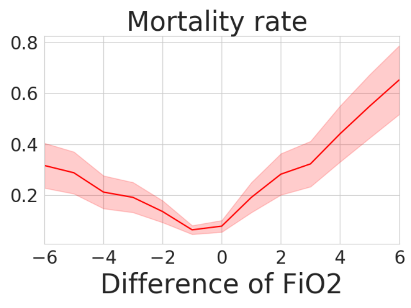


Comparison of Clinician and DAC policies: We find that the mortality rates are lowest in patients for whom clinicians’ actual treatments matched the actions the learned policies recommend. Figure 3 shows the relations between mortality rate and mechanical ventilation setting difference on MIMIC-III. The results show when patients received lower values of FiO2, PEEP and Tidal Volume, the mortality rates increase much faster. We speculate the reasons are two-fold: (i) DAC only recommends high values of FiO2, PEEP and Tidal volume to the high-risk patients, who still have relatively higher mortality rates even with optimal treatments; (ii) the high-risk patients received low-value settings, which further increased their mortality rates.


Policy adaptation: We adapt the model trained on MIMIC-III to AmsterdamUMCdb, and Fig. 4 shows the estimated mortality and WIS with different training sizes on AmsterdamUMCdb. DAC-M is trained on MIMIC-III and directly validated on AmsterdamUMCdb. DAC-A is trained on AmsterdamUMCdb and DACPA is pretrained on MIMIC-III and then adapted to AmsterdamUMCdb. The results show that with transfer learning on AmsterdamUMCdb, DACPA outperforms DAC-M, which demonstrates that the policy adaption is very helpful and improved model performance. When training size becomes smaller, the performance gaps between DACPA and DAC-A are larger, which demonstrates that the introduced policy adaption method is useful when adapting trained models to new-source small-scale datasets.
5. Related Work
In this section, we briefly review the existing works related to DTR and causal inference.
DTR learning. During recent years, there have been some studies that focus on applying RL to the optimal treatment learning from existing (sub)optimal clinical datasets. Komorowski et al. (Komorowski et al. 2018) proposed AI Clinician model which uses a Markov decision process (MDP) to model patients’ health states and learns the treatment strategy to prescribe vasopressors and IV fluids with Q-learning. Raghu et al. (Peine et al. 2021) uses a similar model to AI Clinician to learn the optimal DTR policies for mechanical ventilation and achieves lower estimated mortality rates than human clinicians. (Raghu et al. 2017) expands on Komorowski’s initial work by proposing a Dueling Double Deep Q network Q-learning model with a continuous state space and introduces a continuous reward function to train the model. They show that for patients with higher severity of illness, due to a lack of data, the model did not outperform the human clinicians. (Peng et al. 2018) presents mixture-of-experts (MoE) to combine the restricted DRL approach with a kernel RL approach selectively based on the context and find that the combination of the two methods achieves a lower estimated mortality rate. (Wang et al. 2018) proposes a new Supervised Reinforcement Learning with Recurrent Neural Network (SRL-RNN) model for dynamic treatment regime, which combines the indicator signal and evaluation signal through the joint supervised learning and RL. The experiments demonstrate that the introduced supervised learning is helpful for stably learning the optimal policy. Although the DTR learning algorithms can achieve high performance on treatment recommendation tasks, the learned policies could be biased without the consideration of confounding issues.
DTR learning with causal inference. Causal inference (Greenland et al. 1999; Pearl 2009; Robins et al. 1995) has been used to empower the learning process under noisy observation and can provide interpretability for decision-making models (Schulam and Saria 2017; Bica et al. 2020b; Atan et al. 2018; Bica et al. 2020a; Johansson et al. 2016). In this paper, we focus on the related work of DTR learning with causal inference. Zhang and Schaar (Zhang and van der Schaar 2020) propose a gradient regularized V-learning method to learn the value function of DTR with the consideration of time-varying confounders. Bica et al. (Bica et al. 2020b) present a Counterfactual Recurrent Network (CRN) to estimate treatment effects over time and recommend optimal treatments to patients. Yang et al. (Yang et al. 2021) investigates the resilience ability of an RL agent to withstand adversarial and potentially catastrophic interferences and proposed a causal inference Q-network (CIQ) by training RL with additional inference labels to achieve high performance in the presence of interference. Bica et al. (Bica et al. 2021) propose a counterfactual inverse reinforcement learning (CIRL) by integrating counterfactual reasoning into batch inverse reinforcement learning. From a conceptual point of view, the studies most closely related to ours are (Yang et al. 2021; Bica et al. 2021) and we compare the proposed DAC with them. Both two studies incorporate causal inference into RL models. The key difference between ours and theirs are: (i) we resample the patients and the training DAC with balanced mini-batch can improve the model performance; (ii) we design a short-term reward that can further remove the confounding; (iii) our model is based on actor-critic framework and the critic network can provide more accurate rewards with the help of the patient resampling module and short-term reward; (iv) we introduce a policy adaptation method to the proposed DAC, which can efficiently adapt trained models to new-source environments.
6. Conclusion
In this paper, we investigate the confounding issues and data imbalance problem in clinical settings, which could limit optimal DTR learning performance of RL models. The training of most existing DTR learning methods is guided by the long-term clinical outcomes (e.g., 90 day mortality), so some optimal treatment actions in the history of non-survivors might be punished. To address the issues, we propose a new deconfounding actor-critic network (DAC) for mechanical ventilation dynamic treatment regime learning. We propose a patient resampling module and a confounding balance module to alleviate the confounding issues. Moreover, we introduce a policy adaptation method to the proposed DAC to transfer the learned DTR policies to new-source datasets. Experiments on a semi-synthetic dataset and two publicly available real-world datasets (i.e., MIMIC-III and AmsterdamUMCdb) show that the proposed model outperforms state-of-the-art methods, demonstrating the effectiveness of the proposed framework. The proposed model can provide individualized treatment decisions that could improve patient outcomes.
References
- (1)
- Ambrosino and Gabbrielli (2010) Nicolino Ambrosino and Luciano Gabbrielli. 2010. The difficult-to-wean patient. Expert review of respiratory medicine 4, 5 (2010), 685–692.
- Atan et al. (2018) Onur Atan, James Jordon, and Mihaela van der Schaar. 2018. Deep-treat: Learning optimal personalized treatments from observational data using neural networks. In Proceedings of the AAAI Conference on Artificial Intelligence, Vol. 32.
- Bica et al. (2020a) Ioana Bica, Ahmed Alaa, and Mihaela Van Der Schaar. 2020a. Time series deconfounder: Estimating treatment effects over time in the presence of hidden confounders. In International Conference on Machine Learning. PMLR, 884–895.
- Bica et al. (2020b) Ioana Bica, Ahmed M Alaa, James Jordon, and Mihaela van der Schaar. 2020b. Estimating counterfactual treatment outcomes over time through adversarially balanced representations. arXiv preprint arXiv:2002.04083 (2020).
- Bica et al. (2021) Ioana Bica, Daniel Jarrett, Alihan Hüyük, and Mihaela van der Schaar. 2021. Learning" What-if" Explanations for Sequential Decision-Making. (2021).
- Fan et al. (2017) Eddy Fan, Lorenzo Del Sorbo, Ewan C Goligher, et al. 2017. An official American Thoracic Society/European Society of Intensive Care Medicine/Society of Critical Care Medicine clinical practice guideline: mechanical ventilation in adult patients with acute respiratory distress syndrome. American journal of respiratory and critical care medicine 195, 9 (2017), 1253–1263.
- Gottesman et al. (2018) Omer Gottesman, Fredrik Johansson, Joshua Meier, Jack Dent, Donghun Lee, Srivatsan Srinivasan, Linying Zhang, Yi Ding, David Wihl, Xuefeng Peng, et al. 2018. Evaluating reinforcement learning algorithms in observational health settings. arXiv preprint arXiv:1805.12298 (2018).
- Greenland et al. (1999) Sander Greenland, Judea Pearl, and James M Robins. 1999. Causal diagrams for epidemiologic research. Epidemiology (1999), 37–48.
- Hochreiter and Schmidhuber (1997) Sepp Hochreiter and Jürgen Schmidhuber. 1997. Long short-term memory. Neural computation 9, 8 (1997), 1735–1780.
- Johansson et al. (2016) Fredrik Johansson, Uri Shalit, and David Sontag. 2016. Learning representations for counterfactual inference. In International conference on machine learning. PMLR, 3020–3029.
- Johnson et al. (2016) Alistair E.W. Johnson, Tom J. Pollard, Lu Shen, et al. 2016. MIMIC-III, a freely accessible critical care database. (2016).
- Komorowski et al. (2018) Matthieu Komorowski, Leo A Celi, Omar Badawi, Anthony C Gordon, and A Aldo Faisal. 2018. The artificial intelligence clinician learns optimal treatment strategies for sepsis in intensive care. Nature medicine 24, 11 (2018), 1716–1720.
- Lahouti (2021) Shahriar Lahouti. 2021. Mechanical Ventilation: From Bench to The Bedside Review. (2021). https://recapem.com/mechanical-ventilation-from-bench-to-the-bedside-review/#Acute-Respiratory-failure-(ARF).
- McCaffrey et al. (2013) Daniel F McCaffrey, Beth Ann Griffin, Daniel Almirall, Mary Ellen Slaughter, Rajeev Ramchand, and Lane F Burgette. 2013. A tutorial on propensity score estimation for multiple treatments using generalized boosted models. Statistics in medicine 32, 19 (2013), 3388–3414.
- Mills and Mills (1991) Terence C Mills and Terence C Mills. 1991. Time series techniques for economists. Cambridge University Press.
- Mnih et al. (2015) Volodymyr Mnih, Koray Kavukcuoglu, David Silver, Andrei A Rusu, Joel Veness, Marc G Bellemare, Alex Graves, Martin Riedmiller, Andreas K Fidjeland, Georg Ostrovski, et al. 2015. Human-level control through deep reinforcement learning. nature 518, 7540 (2015), 529–533.
- Pearl (2009) Judea Pearl. 2009. Causality. Cambridge university press.
- Peine et al. (2021) Arne Peine, Ahmed Hallawa, Johannes Bickenbach, Guido Dartmann, Lejla Begic Fazlic, Anke Schmeink, Gerd Ascheid, Christoph Thiemermann, Andreas Schuppert, Ryan Kindle, et al. 2021. Development and validation of a reinforcement learning algorithm to dynamically optimize mechanical ventilation in critical care. NPJ digital medicine 4, 1 (2021), 1–12.
- Peng et al. (2018) Xuefeng Peng, Yi Ding, David Wihl, et al. 2018. Improving sepsis treatment strategies by combining deep and kernel-based reinforcement learning. In AMIA Annual Symposium Proceedings, Vol. 2018. American Medical Informatics Association, 887.
- Prasad et al. (2017) Niranjani Prasad, Li-Fang Cheng, Corey Chivers, Michael Draugelis, and Barbara E Engelhardt. 2017. A reinforcement learning approach to weaning of mechanical ventilation in intensive care units. arXiv preprint arXiv:1704.06300 (2017).
- Raghu (2019) Aniruddh Raghu. 2019. Reinforcement learning for sepsis treatment: Baselines and analysis. (2019).
- Raghu et al. (2017) Aniruddh Raghu, Matthieu Komorowski, Imran Ahmed, Leo Celi, Peter Szolovits, and Marzyeh Ghassemi. 2017. Deep reinforcement learning for sepsis treatment. arXiv preprint arXiv:1711.09602 (2017).
- Robins et al. (1995) James M Robins, Andrea Rotnitzky, and Lue Ping Zhao. 1995. Analysis of semiparametric regression models for repeated outcomes in the presence of missing data. Journal of the american statistical association 90, 429 (1995), 106–121.
- Rosenbaum and Rubin (1983) Paul R Rosenbaum and Donald B Rubin. 1983. The central role of the propensity score in observational studies for causal effects. Biometrika 70, 1 (1983), 41–55.
- Schulam and Saria (2017) Peter Schulam and Suchi Saria. 2017. Reliable decision support using counterfactual models. arXiv preprint arXiv:1703.10651 (2017).
- Sutton et al. (1999) Richard S Sutton, David A McAllester, Satinder P Singh, Yishay Mansour, et al. 1999. Policy gradient methods for reinforcement learning with function approximation.. In NIPs, Vol. 99. Citeseer, 1057–1063.
- Thoral et al. (2020) Patrick Thoral, Jan Peppink, Ronald Driessen, et al. 2020. AmsterdamUMCdb: The First Freely Accessible European Intensive Care Database from the ESICM Data Sharing Initiative. (2020). https://doi.org/10.1109/JBHI.2020.2995139 access: https://www.amsterdammedicaldatascience.nl.
- Tutz and Ramzan (2015) Gerhard Tutz and Shahla Ramzan. 2015. Improved methods for the imputation of missing data by nearest neighbor methods. Computational Statistics & Data Analysis 90 (2015), 84–99.
- Wang et al. (2018) Lu Wang, Wei Zhang, Xiaofeng He, et al. 2018. Supervised reinforcement learning with recurrent neural network for dynamic treatment recommendation. In Proceedings of the 24th ACM SIGKDD International Conference on Knowledge Discovery & Data Mining. 2447–2456.
- Weng et al. (2017) Wei-Hung Weng, Mingwu Gao, Ze He, Susu Yan, and Peter Szolovits. 2017. Representation and reinforcement learning for personalized glycemic control in septic patients. arXiv preprint arXiv:1712.00654 (2017).
- Wunsch et al. (2013) Hannah Wunsch, Jason Wagner, Maximilian Herlim, David Chong, Andrew Kramer, and Scott D Halpern. 2013. ICU occupancy and mechanical ventilator use in the United States. Critical care medicine 41, 12 (2013).
- Yang et al. (2021) Chao-Han Huck Yang, I Hung, Te Danny, Yi Ouyang, and Pin-Yu Chen. 2021. Causal Inference Q-Network: Toward Resilient Reinforcement Learning. arXiv preprint arXiv:2102.09677 (2021).
- Yin et al. (2020) Changchang Yin, Ruoqi Liu, Dongdong Zhang, and Ping Zhang. 2020. Identifying sepsis subphenotypes via time-aware multi-modal auto-encoder. In Proceedings of the 26th ACM SIGKDD international conference on knowledge discovery & data mining. 862–872.
- Zhang et al. (2017) Yutao Zhang, Robert Chen, Jie Tang, Walter F Stewart, and Jimeng Sun. 2017. LEAP: learning to prescribe effective and safe treatment combinations for multimorbidity. In proceedings of the 23rd ACM SIGKDD international conference on knowledge Discovery and data Mining. 1315–1324.
- Zhang and van der Schaar (2020) Yao Zhang and Mihaela van der Schaar. 2020. Gradient Regularized V-Learning for Dynamic Treatment Regimes. Advances in Neural Information Processing Systems 33 (2020).
Appendix A Semi-synthetic dataset based on MIMIC-III
As the MIMIC-III dataset is real-world observational data, it is impossible to obtain the potential outcomes for underlying counterfactual treatment actions. To evaluate the proposed model’s ability to learn optimal DTR policies, we further validate the method in a simulated environment. The treatment assignments at each time stamp are influenced by the confounders , which are consist of hidden confounders and time-varying covariates . We first simulate and for each patient at time following -order autoregressive process (Mills and Mills 1991) as,
| (14) | |||
where and denote the -th column of and , respectively. For each , control the amount of historical information of last p time stamps incorporated to the current representations. controls the influence of previous treatment assignments. are randomly sampled noises.
To simulate the treatment assignments, we generate survivor patients and non-survivor patients. The confounders at time stamp and outcome can be simulated using the hidden confounders and current covariates as follows,
| (15) | ||||
where and . The function maps into the hidden space.
Appendix B Evaluation Metrics
The evaluation metrics for treatment recommendation is still a challenge (Wang et al. 2018; Gottesman et al. 2018). Thus we try different evaluation metrics to compare the proposed model with the state-of-art methods.
Estimated mortality: Following (Wang et al. 2018; Raghu et al. 2017; Weng et al. 2017), we use the estimated in-hospital mortality rates to measure whether policies would eventually reduce the patient mortality or not. Specifically, we train a mortality risk prediction model, which takes the patient states and next actions as inputs, and output mortality risks. The predicted mortality risks are discretized into different units with small intervals shown in the x-axis of Figure 5. Discharged patients dominate both datasets, so the predicted mortality rates are smaller than the actual mortality rate in the real-world clinical setting. We adjusted the predicted mortality rate to calculate a new estimated mortality rate. Given an example denoting an admission of a patient, if the patient died in hospital, all the predicted mortality rates belonging to this admission are associated with a value of mortality and the corresponding units add up these values. After scanning all test examples, the average estimated mortality rates for each unit are calculated, shown in y-axis of Figure 5. Based on these results, the estimated mortality rates corresponding to the predicted mortality rate of different policies are used as the measurements to denote the estimated in-hospital mortality. Although the estimated mortality does not equal the mortality in the real-world clinical setting, it is a universal metric currently for computational testing. The relations between estimated mortality rate and predicted mortality probability are shown in Figure 5.


Weighted importance sampling(WIS): Following (Komorowski et al. 2018; Raghu et al. 2017), we also implement a high-confidence off-policy evaluation (HCOPE) method (WIS). The human clinician policy is defined as , and denotes the learned AI policy. We defined as the per-step importance ratio, where represent the actual (action, state) pair for a patient. is the cumulative importance ratio up to step and denotes the average cumulative importance ratio at horizon in dataset and as the number of trajectories in . The trajectory-wise WIS estimator is given by:
| (16) |
where denotes the length of steps for the patient and denote the long-term reward. Then, the WIS estimator is the average estimate over all trajectories, namely:
| (17) |
where is WIS applied to the trajectory for patient.




Action accuracy rate: Following (Bica et al. 2021; Yang et al. 2021), we compute the optimal action accuracy rate to evaluate the models’ performance to learn optimal DTR policies in simulated environments. Mechanical ventilator has three important parameters: PEEP, Vt and FiO2. We compute two kinds of accuracy rates: ACC-3 (whether the three parameters are set the same as the optimal action simultaneously) and ACC-1 (whether each parameter is set correctly). The metrics are computed as follows:
| (18) |
where , , are recommened actions for PEEP, Vt and FiO2, , , are optimal actions.
Appendix C Additional Experimental Results
The relations between expected returns and mortality rates are shown in Figure 8. The results show that our model has a more clear negative correlation between expected returns and mortality rates than DQN in both MIMIC-III and AmsterdamUMCdb datasets. The reason might be two-fold: (i) DQN is trained on the initial EHR data with confounder bias; (ii) DQN punishes the actions used for patients who suffer from mortality, while some actions might be optimal.


Distribution of Actions: Visualization of the action distribution in the 3-dimensional action space on AmsterdamUMCdb are shown in Figure 6. The results show that the proposed model learned similar policies to clinicians. DAC suggests more actions with the lowest and highest PEEP and FiO2. Besides, the learning policies recommend more frequent lower tidal volume compared to clinician policy.
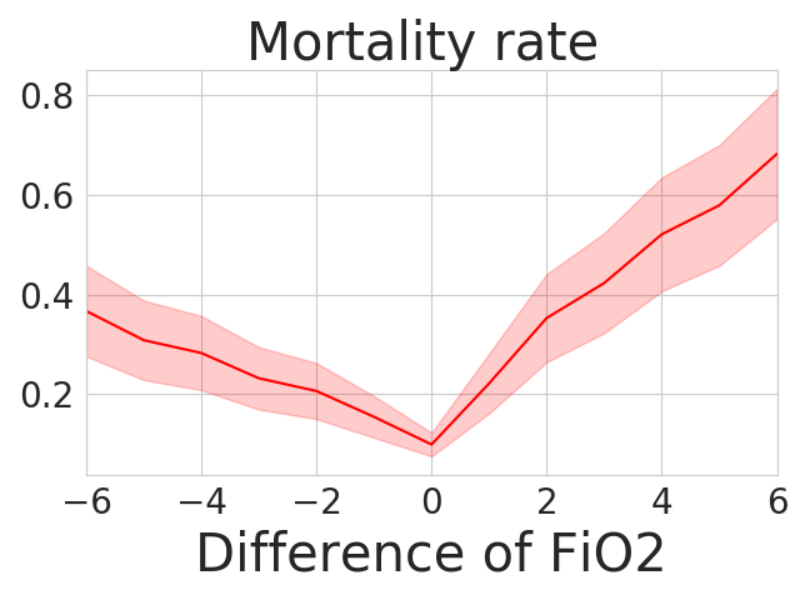
Comparison of Clinician and DAC policies: We find that the mortality rates are lowest in patients for whom clinicians’ actual treatments matched the actions the learned policies recommend both on MIMIC-III and AmsterdamUMCdb datasets. Figure 7 shows the relations between mortality rate and mechanical ventilation setting difference on AmsterdamUMCdb.
Hyper-parameter optimization: Figure 9 shows the optimization of parameter on MIMIC-III dataset. We find the model performance is not sensitive when . We set when training the DAC model. Because the long-term rewards’ value range (i.e., from -15 to +15) is wider than short-term rewards’ value range (i.e., from -1 to +1), the weight of long-term reward is smaller than the weight of short-term reward.