A Local Wheeler-DeWitt Measure

We embrace the notion of de Sitter space as a quantum mechanical system with a finite-dimensional Hilbert space [48, 57, 63, 64]. Based on this, we want to develop a simple toy model for eternal inflation, which is most naively understood as a sequence of tunneling transitions between several such de Sitter vacua.²² 2 As will be discussed later on, the Schrödinger equation should in fact be replaced by the Wheeler-DeWitt (WDW) equation. For the moment we assume that (in some approximation) we can instead use a conventional Hamiltonian and a time variable defined e.g. by some physical system (a clock) [57, 48, 65, 58]. A more detailed analysis will be given in Sections 3 and 4. The Hilbert space $\cal H$ of a single dS vacuum is of dimension $N\simeq\exp(S)$, where $S\simeq\pi(RM_{P})^{2}$ denotes the entropy of the horizon. We expect the energy eigenvalues of our dS space to form a very dense discretuum, at least in the energy range that corresponds to what we view as semiclassical de Sitter space. It then makes sense to introduce the continuous function $N(E)$ characterizing the number of states below an energy $E$ asymptotically, in a distributional sense. We also introduce the density of states $\rho(E)=dN(E)/dE$. Since there are only finitely many energy levels, $N$ and $N(E)$ clearly coincide for large enough $E$. In this notation, the semiclassical dS states lie in a region of high density, presumably, their energies are close to $E_{*}$ with $E_{*}$ being defined as the value where $\rho(E)$ is maximal. A small subsystem inside a dS space in a semiclassical state sees a temperature $T\sim 1/R$. The density of states at $E_{*}$ can then be computed using standard thermodynamic relations:

$$\frac{1}{R}\sim T=\left.\frac{dE(S)}{dS}\right|_{E_{*}}=\left.\frac{dE(S)}{d\log(N(E))}\right|_{E_{*}}=N(E_{*})\left.\frac{dE(N)}{dN(E)}\right|_{E_{*}}=\frac{N(E_{*})}{\rho(E_{*})}\,.$$

(2)

Solving for $\rho(E_{*})$ yields

$$\rho(E_{*})\sim RN(E_{*})\,.$$

(3)

We naturally expect that $N(E_{*})\sim N$. If we are willing to neglect sub-exponential terms, we may simply write

$\displaystyle\rho(E_{*})\sim N\,.$

(4)

Note that this fixes the density of states in the energy range $E\sim E_{*}$ relevant for semiclassical dS, but it does not fix the precise value of $E_{*}$. The latter is not relevant in our context.

Now, we allow for a second dS minimum, such that we can label the two dS vacua as false and true respectively. Our Hilbert space is then the direct sum of two subspaces of dimensions $N_{f}$ and $N_{t}$, where the index stands for true or false. We assume that $N_{f}\ll N_{t}$ and that tunneling transitions can occur. The total Hamiltonian takes the form

$$H=\left(\begin{array}[]{cc}H_{f}&\Delta\\ \Delta^{\dagger}&H_{t}\end{array}\right)\,,$$

(5)

where the $(N_{f}\times N_{t})$-matrix $\Delta$ is assumed to have extremely small entries of typical size $\delta$.

We want to determine which $\delta$ matches the semiclassical expectation for the decay rate of a generic state in ${\cal H}_{f}$. In the field-theoretic regime, this rate is given by the Coleman-De Luccia (CDL) result [66] $\Gamma_{sc}\simeq R_{f}^{3}\exp(-B)=R_{f}^{3}\exp(-S_B+S_A)$, with $S_{B}$ the action of the $O(4)$-symmetric bounce and $S_{A}$ the action of the false vacuum. The probability for a quantum state being in ${\cal H}_{f}$ then decays in the standard exponential way: $p_{t}\sim\exp(-\Gamma_{sc} t)$.³³ 3 It would be very interesting to also consider de Sitter minima which are connected by paths through flat scalar potentials, such that Hawking-Moss (HM) [67] transitions become relevant. Also, for pairs of vacua that are not connected by an instanton, non-tunneling transitions [68] have to be considered. We leave this subject to future work.

To make progress, we now introduce a key assumption, illustrated in Fig. 1: We assume that the interval in which the energy eigenvalues of $H_{f}$ are mainly distributed lies inside the high-density region of the $H_{t}$ spectrum. As a result, the tunneling probability does not depend on which particular state of the false vacuum we are starting from. This agrees with semiclassical expectations since the large number of states comes from the horizon degrees of freedom, and the latter should not influence the semiclassical bubble formation probability of CDL.

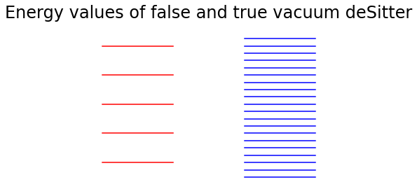
Under the assumption above, $\rho_{t}$ is very large in the relevant energy range and a typical ${\cal H}_{f}$ state decays into a quasi-continuum. The rate in our quantum-mechanical toy model then follows Fermi’s Golden Rule:

$$\Gamma_{qm}\sim\delta^{2}\rho_{t}\,.$$

(6)

Demanding $\Gamma_{qm}=\Gamma_{sc}$ allows us to estimate $\delta$ (disregarding non-exponential effects) as

$$\delta^{2}\sim\exp(-B)/\rho_{t}\,.$$

(7)

We note that the standard derivation of Fermi’s Golden Rule relies on a continuum approximation for the spectrum of the final-state subspace. This limits the validity to a time range below $T_{max}\sim 1/\rho_{t}$. If we want our false vacuum to actually decay within the time range we control, we need $\Gamma_{qm}\gtrsim 1/T_{max}$, which implies

$$\rho_{t}\,\delta\gtrsim 1\,.$$

(8)

The same constraint follows from a static perspective: Namely, we should demand that any eigenstate of the full system mostly points in the ${\cal H}_{t}$ part of the total Hilbert space. If this were not the case, one could prepare the system in an eigenstate pointing mostly in ${\cal H}_{f}$ and forever observe it in the false vacuum. This contradicts the semiclassical expectation that the false vacuum eventually has to decay. A necessary condition for our claim is that perturbation theory in $\delta$, correcting the original eigenstates of $H_{f}$, should break down. At leading order, the square of the ${\cal H}_{t}$-projection of a corrected $H_{f}$-eigenvector is estimated by

$$\sum_{E_{t}}\frac{\delta^{2}}{(E_{f}-E_{t})^{2}}\,.$$

(9)

This sum is dominated by the term that contains the eigenvalue $E_{t}^{0}$ which lies closest to $E_{f}$. We naturally expect that $E_{f}-E_{t}^{0}\sim 1/\rho_{t}$ (for an accidental resonance $E_{f}=E_{t}^{0}$, the cutoff at $T_{max}$ prevents a pole) such that the sum (9) may be approximated by $\delta^{2}\rho_{t}^{2}$. Requiring this to be of order unity or larger is equivalent to (8).

In our specific case of CDL tunneling, we have $\delta\sim\exp(-B)$ and $\rho_{t}\sim\exp(S_t)$, such that (8) turns into the condition

$$B\lesssim S_{t}\,.$$

(10)

In fact, a general argument [6] shows that instantonic tunneling transitions between dS vacua always obey

$\displaystyle B\leq S_{dS}\,,$

(11)

with $S_{dS}$ being the entropy of the decaying dS. This is consistent with expectations that dS spaces do not live longer than their recurrence time $t_{rec}\simeq\exp(S_{dS})$ [45, 69]. Since $S_{f}\leq S_{t}$, it is immediately clear that (11) implies (10). The fact that the relevant bound (10) holds on such general grounds encourages us to think that our basic picture of finite-dimensional Hilbert spaces, linked by decays into a quasi-continuum, is sensible.

We note that certain decay rates may violate our bound, e.g. the non-tunneling transitions of [68]. This does not represent a problem for our approach since there is no reason to expect that dS spaces exist which decay exclusively via such extremely slow transitions.

We expect the overwhelming majority of eigenvectors to deviate only very little from the $\mathcal{H}_{t}$ subspace of the Hilbert space $\mathcal{H}_{t}\oplus\mathcal{H}_{f}$. To quantify this, we consider two general classes of models. First, we draw an analogy to classical mechanics: Our full Hilbert space with a Hamiltonian of the form (5) may be compared to a classical system the phase space of which is the union of two distinct subspaces. Moreover, transitions between these subspaces are suppressed. For example, one may think of a particle in a large container with a peculiar geometry: Namely, it should be the union of two smaller containers connected by a short and narrow throat.

Now, we know that a particle in an irregular, compact geometry in general represents an ergodic system. In other words, integrating over a long period of time the (appropriately averaged) distribution of the particle position on a fixed-energy phase space slice is constant. Moreover, the Shnirelman theorem [70] extends this statement to quantum mechanics. Specifically, it states that for a manifold with ergodic geodesic flow, the probability density associated to an eigenfunction of the Laplacian will generically, in the limit of large eigenvalues, tend towards the uniform distribution in phase space.

In principle, the Shnirelman theorem applies also to our geometry of interest, where the configuration space manifold consists of two well-separated regions connected by a narrow throat. However, in practice one is of course not interested in asymptotically high-energy eigenfunctions but rather hopes that the statement of the theorem holds with sufficient precision above a certain moderate energy threshold. The problem in our case is that this energy threshold presumably grows as the throat becomes more and more narrow. This narrowness is related to the smallness of $\delta$ in (5). While it would be interesting to investigate the relevant limiting procedures more carefully, this would in itself not suffice to establish the applicability of Shnirelman’s theorem. The reason is that there is another even more obvious obstacle: The Shnirelmann theorem, as it stands, only applies to infinite-dimensional Hilbert spaces where the Hamiltonian is an elliptic operator, for example the Laplacian. Our system of interest has by definition a finite Hilbert space to start with. Moreover, we do not know whether it can be derived in some way from a related classical system.

Thus, the best we can do for now is to take the Shnirelman theorem as an inspiration and to proceed from the expectation that an analogous statement holds for our model Hamiltonian (5). Our main motivations are the very large dimensions of the relevant subspaces and the expected random behaviours of the spectra of $H_{f,t}$ as well of the entries of the transition matrix $\Delta$. To formlate our expectation quantitatively, we denote the norm of the projection of a vector on the $\mathcal{H}_{f,t}$ part of the total Hilbert space by $\|\cdot\|_{f,t}$. Now the claim that the probability density associated to an eigenvector tends towards the uniform distribution in phase space translates to the statement that, for a generic normalized eigenvector $v$ of $H$, one has

$$\|v\|_{f}^{2}\simeq\frac{N_{f}}{N_{f}+N_{t}}\,\,,\qquad\|v\|_{t}^{2}\simeq\frac{N_{t}}{N_{f}+N_{t}}\,.$$

(12)

Here, the squared norms of the projections of $v$, i.e. the left-hand sides in the two relations in (12), correspond to the probability distributions associated to $v$ in Shnirelman’s sense. The right hand sides represent the relative sizes of the dimensions of the Hilbert subspaces, which corresponds to the claim of equidistribution in phase space volume.

The same result can be obtained using a second, totally different approach, based on different assumptions. To motivate it, recall that depending on the size of $\delta$ our system is found in two distinct regimes: For small $\delta$, perturbation theory in $\delta$ works and the $N_{f}+N_{t}$ eigenvectors split in two subsets – $N_{f}$ of them lie mostly in ${\cal H}_{f}$, the other $N_{t}$ lie mostly in ${\cal H}_{t}$. The strong assumption we now make is that, when $\delta$ is not very small, the exact eigenvector basis is given by a randomly chosen orthonormal basis in ${\cal H}_{t}\oplus{\cal H}_{f}$. We may specify this proposal by stating that our basis is the eigenbasis of a random hermitian matrix, as analysed in [71, 72]. The results of [71, 72] concerning the eigenvector distribution can be stated as follows: For a normalized eigenvector $v$ of a random hermitian matrix, the quantity $\|v\|_{f,t}^{2}$ is, in the large $N_{f}+N_{t}$ limit, Gaussian distributed with mean and variance

$$\mu_{f,t}=\frac{N_{f,t}}{N_{f}+N_{t}}\,\,\,,\qquad\sigma^{2}_{f,t}\sim\frac{N_{f,t}}{(N_{f}+N_{t})^{2}}\,.$$

(13)

In the limit of large $N_{f}$ and $N_{t}$, we see that the distribution of $\|v\|_{f,t}^{2}$ is sharply peaked around $\mu_{f,t}$. This is in perfect accordance with the proposal (12) motivated using Shnirelman’s theorem. Thus, whenever one de Sitter vacuum has an appreciably higher cosmological constant than the other, $N_{t}$ is exponentially larger than $N_{f}$, and hence $\|v\|_{f}^{2}$ will be exponentially small for a generic normalized eigenvector $v$. This conforms with the semiclassical expectation that the false vacuum unavoidably decays.

More specifically, we want to take the point of view of an observer in our landscape of two vacua and ask which vacuum they expect to find themselves in. In our approach, they can make a prediction by taking the solution of the Schrödinger equation describing their universe and projecting on one or the other vacuum. The most general solution is of the form

$\displaystyle\Psi=\sum_{i=1}^{N_{t}+N_{f}}a_{i}\exp(i\lambda_i t)v_{i}\,,$

(14)

where $\lambda_{i}$ are the eigenvalues of the full Hamiltonian and $v_{i}$ are the corresponding normalized eigenvectors. The complex coefficients $a_{i}$ parameterize the family of solutions. The probability with which an observer sees the false vacuum is then given by

$\displaystyle R_{qm}=\frac{\int dt\|\Psi\|_{f}^{2}}{\int dt\|\Psi\|^{2}}=\frac{\sum_{i=1}^{N_{f}+N_{t}}\|v_{i}\|_{f}^{2}|a_{i}|^{2}}{\sum_{i=1}^{N_{f}+N_{t}}|a_{i}|^{2}}\simeq\frac{N_{f}}{N_{f}+N_{t}}\,.$

(15)

Here the last, approximate equality holds only for a generic solution or, more precisely, it is the expectation for an arbitrary but fixed choice of the $a_{i}$. Our quantum-mechanical result $R_{qm}$ may be compared with the semiclassical prediction based on following a single observer through the multiverse and integrating the times they spend in each vacuum [46, 73]

$\displaystyle R_{sc}\sim\frac{\exp(-24\pi^2M_P^2/\Lambda_f)}{\exp(-24\pi^2M_P^2/\Lambda_f)+\exp(-24\pi^2M_P^2/\Lambda_t)}\sim\frac{N_{f}}{N_{f}+N_{t}}\,.$

(16)

This result was derived from rate equations describing an infinite sequence of CDL tunneling events. It agrees with the prediction of our quantum mechanical toy model at the level of exponentially large terms.

As noted in [46], the non-exponential prefactors associated with the tunneling rates violate ergodicity, which in our approach is the basic starting point. At the technical level, this is not an immediate problem for us: On the one hand, we take the quantum mechanical picture more seriously than the semiclassical perspective of following a single observer’s worldline. On the other hand, our present work merely attempts to outline an approach that works in principle – we are happy to accept sub-exponential errors. Nevertheless, it would be interesting to pursue this apparent non-ergodicity issue in more detail. For example, our suggestion for a generalized Shnirelman theorem may have sub-exponential errors. It is also conceivable that the tunneling rate has corrections reinstating ergodicity (although we understand that the authors of [46] dismiss this option).

We called the discussion of Sect. 2 ‘naive’ for an obvious reason: We are dealing with a time reparameterization invariant theory and the Schrödinger equation is hence not the appropriate tool. Instead, one has to use the Wheeler-DeWitt (WDW) equation [55] (see [75] for a review),

$$H{\Psi}=0\,.$$

(17)

While the wave function of the universe $\Psi$ is by definition time-independent, the concept of time naturally arises from correlations between observables.

We find it convenient to start with a particularly simple toy model - a point-particle moving in $d$-dimensional Minkowski space. Its Polyakov action reads

$\displaystyle S=\int d\tau\,\left(\gamma^{-1}\dot{X}^{\mu}(\tau)\dot{X}^{\nu}(\tau)\eta_{\mu\nu}-\gamma\left(m^{2}+V\left(X^{i}(\tau)\right)\right)\right)\,,$

(18)

where $X^{\mu}$ are the target space coordinates, $\gamma(\tau)$ is the square root of the worldline metric (the einbein), and $V(X^{i})$ is a potential in which the particle is trapped. For simplicity, $V$ does not depend on $X^{0}$. From the reparameterization invariance of $\tau$, one derives a constraint which, after quantization, takes the form

$$H\Psi(X^{\mu})=0\qquad\mbox{with}\qquad H=\frac{1}{2}(-\partial_{\mu}\partial^{\mu}+m^{2}+V(X^{i}))\,.$$

(19)

From the WDW perspective, the coordinate $X^{0}$ is set apart since it enters the equation with a wrong-sign kinetic term. Since $V$ does not depend on $X^{0}$, a product ansatz of the form $\Psi(X^{\mu})=\exp(\pm ikX^0)\chi(X^{i})$ can be made. This leads to a time-independent Schrödinger equation for $\chi$:

$\displaystyle(-\partial_{i}\partial^{i}+m^{2}+V(X_{i}))\chi(X^{i})=k^{2}\chi(X^{i})\,.$

(20)

We see that, not only in target space but also in the resulting quantum mechanical system, $X^{0}$ plays the role of time. The only special feature is the appearance of positive and negative frequency modes – a consequence of the WDW equation being second rather than first order in $\partial_{0}$.

On the space of wavefunctions $\Psi(X^{\mu})$, a natural scalar product is given by

$\displaystyle(\Psi,\Phi)=\int\mathrm{d}^{d}X\,\Psi^{*}\Phi\,.$

(21)

However, the subspace of solutions to (19) is in addition equipped with an alternative inner product. To see this note that (19) is (a slightly modified version of) the Klein-Gordon equation, implying that the current

$\displaystyle j^{\mu}=\frac{i}{2}\left(\Psi\partial^{\mu}\Psi^{*}-\Psi^{*}\partial^{\mu}\Psi\right)$

(22)

is conserved. This allows for the definition of the Klein-Gordon inner product

$\displaystyle(\Psi,\Phi)_{KG}=\int_{\Sigma}\frac{i}{2}\left(\Phi\partial_{\mu}\Psi^{*}-\Psi^{*}\partial_{\mu}\Phi\right)\mathrm{d}A^{\mu}\,.$

(23)

Crucially, assuming appropriate boundary conditions, this is independent of the choice of the spacelike codimension-one submanifold $\Sigma$ over which the current is integrated. However, taking (23) as the Hilbert space inner product of the quantum theory has issues. The first one is the well-known fact that (23) is only positive definite if restricted to positive frequency solutions. The second problem is related to calculating expectation values of operators $O$. In general, $O\Psi$ does not satisfy (19), implying that a current analogous to (22) but including $O$,

$\displaystyle j^{\mu}=\frac{i}{2}\left((O\Psi)\partial^{\mu}\Psi^{*}-\Psi^{*}\partial^{\mu}(O\Psi)\right)\,,$

(24)

is not conserved. As a result, $(\Psi,O\Psi)_{KG}$ depends on the chosen hypersurface $\Sigma$. To illustrate this, consider (19) in $1+1$ dimensions with vanishing mass and potential. Then, a simple wave packet,

$\displaystyle\Psi(X^{0},X^{1})=\exp(-(X^1-X^0)^2+ik_0(X^1-X^0))\,,$

(25)

represents a solution. We should be able to predict the most likely value of $X^{1}$ when $X^{0}$ takes values between $X^{0}_{a}$ and $X^{0}_{b}$. Put differently, we want to calculate the expectation value of $P^{0}_{ab}X^{1}$, where $P^{0}_{ab}$ is the operator projecting the wavefunction to the strip $X^{0}\in(X^{0}_{a},X^{0}_{b})$. Using (21), we find the intuitive result

$\displaystyle(\Psi,P^{0}_{ab}X^{1}\Psi)=\int_{X^{0}_{a}}^{X^{0}_{b}}\!\!dX^{0}\,\int_{-\infty}^{\infty}\!\!dX^{1}\,X^{1}\exp(-2(X^1-X^0)^2)=\frac{\sqrt{2\pi}}{4}(X^{0}_{b}-X^{0}_{a})(X^{0}_{b}+X^{0}_{a})\,.$

(26)

By contrast, the Klein-Gordon inner product with $\Sigma$ chosen to be the hypersurface $X^{0}=\,$const. gives ⁴⁴ 4 For $k_{0}\gg 1$, the wave packet (25) contains essentially only positive frequency modes, such that the issue of non-positive-definiteness is absent.

$\displaystyle(\Psi,P^{0}_{ab}X^{1}\Psi)_{KG}=\begin{cases}0&\textbf{if }X^{0}\notin(X^{0}_{a},X^{0}_{b})\\ \int dX^{1}\,k_{0}X^{1}\exp(-2(X^1-X^0)^2)=\sqrt{\frac{\pi}{2}}k_{0}X^{0}&\textbf{if }X^{0}\in(X^{0}_{a},X^{0}_{b})\end{cases}\,.$

(27)

We observe that (27) depends on the chosen value of $X^{0}$, which is expected since $P^{0}_{ab}X^{1}\Psi$ does not solve (19). Of course, to obtain a result independent of $X^{0}$ one may consider averaging (27) over all hypersurfaces $X^{0}=\,$const. within the prescribed interval. But this appears ad hoc and goes against the key idea that the Klein-Gordon inner product should be hypersurface-independent.

The problem of $(\Psi,O\Psi)_{KG}$ not being well defined occurs generally for operators that do not commute with $H$, which is the case for most operators of practical interest. This lends support to the use of (21) rather than (23).

A more relevant model for us is the mini-superspace description of an FLRW spherical geometry with scale factor $a=\exp(\alpha)$, curvature $k$, as well as a (homogeneous) scalar field $\phi$ in a potential $V(\phi)$. The appropriately truncated Einstein-Hilbert action reads [55, 60]

$$S=\int\differential t\left[-e^{-3\alpha}\dot{\alpha}^{2}+ke^{\alpha}+e^{3\alpha}\dot{\phi}^{2}-e^{3\alpha}V(\phi)\right],$$

(28)

showing that this time the scale factor plays the special role of the variable with the wrong-sign kinetic term. The resulting WDW operator takes the form

$$H=\frac{1}{2}\left[e^{-3\alpha}\left(\partial_{\alpha}^{2}+p^{\prime}(\alpha)\partial_{\alpha}-\partial_{\phi}^{2}\right)+e^{3\alpha}\left(V(\phi)-ke^{-2\alpha}\right)\right]\,,$$

(29)

where the function $p(\alpha)$ parameterizes an operator ordering ambiguity [76, 60]:

$$e^{-p(\alpha)}\pi_{\alpha}e^{p(\alpha)}\pi_{\alpha}\quad\to\quad-e^{-p(\alpha)}\partial_{\alpha}\left(e^{p(\alpha)}\partial_{\alpha}\right)\,.$$

(30)

In the late-time, semiclassical regime (i.e. $\alpha\to\infty$), the WDW equation simplifies to

$$0=\left[e^{-3\alpha}\left(\partial_{\alpha}^{2}-\partial_{\phi}^{2}\right)+e^{3\alpha}V(\phi)\right]\Psi(\alpha,\phi)\,.$$

(31)

In analogy to (21), one may use the scalar product

$$\left\langle\Psi_{1}\middle|\Psi_{2}\right\rangle=\int d\phi\int_{-\infty}^{\infty}\mathrm{d}\alpha\,e^{3\alpha}\,\Psi_{1}^{*}(\alpha,\phi)\Psi_{2}(\alpha,\phi)\,,$$

(32)

where the factor $e^{3\alpha}$ ensures that the WDW operator is self adjoint [76, 60].

Alternatively, one could have tried to use the DeWitt inner product [55] on the space of solutions to (31), which is defined in analogy to the Klein-Gordon inner product (23), and has recently proven to be a useful tool in holographic computations [77, 78]. As in the Klein-Gordon case, one faces the issue of non-positive-definiteness. Although a probability interpretation can nevertheless be given in special situations, e.g. when working in the WKB approximation where the wavefunction can be decomposed in positive and negative frequency parts, it is not clear how the DeWitt product can be used in more general setups [75, 79, 80, 81]. Moreover, operators corresponding to observables of interest, such as the counting of galaxies at large $\alpha$, fail to commute with $H$. Thus, as in the Klein-Gordon case, making their expectation values well-defined would require an ad-hoc average over hypersurfaces.

Our preferred inner product definition (32), which one may call the ‘Hartle-Hawking inner product’ [74], can be applied before restricting to solutions of (31) and before gauge fixing. One of its main known problems are divergences arising in the integration over the entire parameter space. We give two arguments in its defense: First, even if the integral in (32) is divergent, one may still be able to derive finite relative probabilities. Second, in a theory with a finite-dimensional Hilbert space, which is what we are after eventually, the problem of diverging integrals is presumably entirely absent. Finally, we note that divergent integrals may also arise when using the DeWitt inner product to calculate expectation values, namely in the process of averaging over hypersurfaces.

By comparison with the point particle example above, it now appears very natural to think of $\alpha$ as a time variable [82, 83]. One may then encode a (toy-model) landscape in a set of minima of $V(\phi)$ and try to approach the measure problem in the resulting mini-superspace framework. Such an approach has in fact already been pursued in [53, 31, 52]⁵⁵ 5 We found the explicit solutions of toy-model WDW equations with concrete scalar-field potentials in [52] more convincing than the general analysis of [53, 31]. However, as will be explained in the main text, we have conceptual issues with this framework independently of the technical implementation. and [54]. To be precise, only [53, 31, 52] refer directly to the WDW equation while [54] appears to be closer to what we called ‘naive quantum-mechanical’ approach. Both references appeal to Anderson localization [84] to make statements about the wave function of the universe.

We see conceptual issues with the straightforward use of the mini-superspace model based on $\alpha$ and $\phi$ advocated in [53, 31, 52]. The problem is that Coleman-De Luccia instantons and the subsequently expanding bubbles violate global homogeneity of the spatial 3-sphere. But this was a key assumption underlying the model. Put differently, tunneling in the mini-superspace model corresponds to transitions where the whole spatial $S^{3}$ changes the vacuum state at once. But this is not what happens according to Coleman-De Luccia and it is inconsisent with causality at late times, when the 3-sphere is much larger than the horizon.

By contrast, Ref. [54] focuses on a single Hubble patch of a dS space and analyzes the scalar-field dynamics resulting from the nonzero temperature of the dS. The starting point is the Langevin equation (derived in this context by Starobinsky [85]). From this, an effective Schrödinger-type equation can be obtained, to which Anderson’s findings are eventually applied. The problem with this approach is that the Langevin equation is only derived in a regime where the slow roll conditions hold, but the later analysis makes statements about the entire landscape (where we do not expect transitions between different minima to occur in the slow roll regime). Still, it may in principle be possible and worthwhile to compare our results with those of [54] in a restricted setting where both are applicable.

Let us now try to develop an alternative suggestion for a WDW equation in a landscape situation, avoiding the apparent shortcomings of earlier approaches just discussed. As already noted at the very beginning of Sect. 3, our results will still not be satisfactory and we will eventually turn to an improved, more minimalist point of view in Sect. 4.

Crucially, we can not use a mini-superspace modelling the whole spatial $S^{3}$ since we assume that only the spacetime inside the horizon is real. The wave function ${\Psi}$ of the universe hence describes a superposition of different vacua in a single static patch. In general, the static patch looks homogeneous and isotropic to the observer sitting at the center. This homogeneity is broken if a bubble of a new vacuum nucleates, but it is restored very quickly as the de Sitter expansion continues in the new vacuum. Thus, one may hope that a quantum description similar to the mini-superspace approach exists. To write down an appropriate Hamiltonian, we may take (31) as an inspiration. However, there appears to be no justification for the relative exponential factors between $\partial_{\phi}^{2}$ and $V(\phi)$ since the local $\phi$-field dynamics inside the horizon is not modified in the course of the ongoing exponential expansion. Let us then, in a first attempt, drop the exponential factors altogether and consider the WDW Hamiltonian

$$H=\partial_{\alpha}^{2}+H_{\phi}\,,$$

(33)

acting on the Hilbert space⁶⁶ 6 We view (33) as some form of ‘continuum approximation’ to the true Hamiltonian acting on the finite-dimensional space (34).

$\displaystyle\mathcal{H}_{dS}=\mathcal{H}_{bulk}\otimes\mathcal{H}_{horizon}\,,\qquad\quad(\,\,\mbox{with}\,\,\,\,\dim\mathcal{H}_{dS}=\exp(S_{dS})\,\,)\,,$

(34)

of the static-patch observer. This tensor product ansatz is inspired, among others, by [32, 47]. In the simplest mini-superspace model, $H_{\phi}=-\partial_{\phi}^{2}+V(\phi)$. More generally, the Hamiltonian $H_{\phi}$ should describe the dynamics of all scalar-field and gravitational fluctuations of the static patch. These degrees of freedom are encoded in $\mathcal{H}_{bulk}$, which is hence subject to the action of $H_{\phi}$. It remains at this stage unclear to which extent and how $H_{\phi}$ also acts on $\mathcal{H}_{horizon}$. Some form of non-trivial action of $H_{\phi}$ on $\mathcal{H}_{horizon}$, which of course contains the majority of degrees of freedom of the entire system [86], is presumably required. The variable $\alpha$ is interpreted as living in $\mathcal{H}_{horizon}$ and encoding a remnant of the semiclassical expansion of the global dS sphere which, of course, we have abandoned. Hence, the operator $\partial_{\alpha}^{2}$ acts only on the space $\mathcal{H}_{horizon}$.

We note that the approximate factorization in bulk and horizon degrees of freedom assumed in (34) relies on the limit of weak gravity, $1/M_{P}^{2}\to 0$. It is strongly broken if the bulk region contains so much energy that the size of the horizon shrinks significantly. This happens e.g. for black hole states close to the Nariai limit.

Comparing the Hamiltonian (33) with that in (19) and the subsequent analysis, it becomes apparent that $\alpha$ plays the role of a time variable. We may furthermore attempt to identify $H_{\phi}$ with the Hamiltonian (5) of our toy-model quantum mechanical description. But such an identification is not perfect since some of the degrees of freedom are already encoded in $\alpha$.

Unlike in (14), solutions of the WDW equation are now composed of positive and negative frequency parts

$\displaystyle\Psi(\alpha)=\sum_{i=1}^{N_{t}+N_{f}}\left(a_{i}\exp(i\sqrt{\lambda_i} \alpha)+b_{i}\exp(-i\sqrt{\lambda_i} \alpha)\right)v_{i}\,,\quad a_{i},b_{i}\in\mathbb{C}\,.$

(35)

We would like to argue that, nevertheless, the crucial calculation (15) remains essentially unchanged:

$\displaystyle R_{qm}=\frac{\int d\alpha|\Psi|_{f}^{2}}{\int d\alpha|\Psi|^{2}}=\frac{\sum_{i=1}^{N_{f}+N_{t}}\|v_{i}\|_{f}^{2}\left(|a_{i}|^{2}+|b_{i}|^{2}\right)}{\sum_{i=1}^{N_{f}+N_{t}}\left(|a_{i}|^{2}+|b_{i}|^{2}\right)}\sim\frac{N_{f}}{N_{f}+N_{t}}\,,$

(36)

Concerning the first two equalities this is obvious. However, arguing for the approximate result $N_{f}/(N_{f}+N_{t})$ after the last step is problematic. Originally, we arrived at this relation by generalizing Shnirelman’s theorem and assuming $\|v_{i}\|_{f}^{2}/\|v_{i}\|_{t}^{2}\sim N_{f}/N_{t}$ for a generic eigenvector $v_{i}$ in ${\cal H}_{t}\oplus{\cal H}_{f}$. In our present setting we would have to generalize (34) according to

$${\cal H}_{tot}={\cal H}_{t}\oplus{\cal H}_{f}=\Big(\mathcal{H}_{bulk}^{t}\otimes\mathcal{H}_{horizon}^{t}\Big)\,\oplus\,\Big(\mathcal{H}_{bulk}^{f}\otimes\mathcal{H}_{horizon}^{f}\Big)$$

(37)

to make this argument.

The difficulty is now that our variable $\alpha$ somehow has to belong to the two horizon Hilbert spaces $\mathcal{H}_{horizon}^{t}$ and $\mathcal{H}_{horizon}^{f}$ together. Even worse, in a more realistic case there would be as many such Hilbert spaces as there are dS vacua and our single variable $\alpha$ has to be encoded in all of them at the same time. Even though this sounds maybe surprising, it is certainly conceivable.

Alternatively, we may try to abandon the idea of deriving the last relation in (36) using Shnirelman’s theorem. Then, we can speculate that the Hamiltonian $H_{\phi}$ only acts on states in $\mathcal{H}_{bulk}$. The action of (33) then factorizes according to the product structure $\mathcal{H}_{bulk}\otimes\mathcal{H}_{horizon}$ of our full Hilbert space. While the Shnirelman theorem now can not be used to argue for the result (36), we may appeal to the more conventional approach of looking for stationary solutions of tunneling rate equations [46, 73]. As discussed around (16), this gives the same result: $R_{sc}\sim R_{qm}\sim N_{f}/(N_{f}+N_{t})$. In this case, the appropriate generalization of (34) would be

$${\cal H}_{tot}=\Big({\cal H}_{bulk}^{t}\oplus{\cal H}_{bulk}^{f}\Big)\otimes{\cal H}_{horizon}\,.$$

(38)

However, it then remains unclear how exactly to think about ${\cal H}_{horizon}$. After all, its dimension depends on the cosmological constant associated with the bulk, the latter in general being very different between true and false vacuum.

Furthermore, we note that following [47] one might also imagine that additional degrees of freedom are present behind the horizon, encoded in a Hilbert space $\mathcal{H}_{*}$. In this case, (34) has to be replaced by

$${\cal H}_{dS}={\cal H}_{bulk}\otimes{\cal H}_{horizon}\otimes{\cal H}_{*}\,,$$

(39)

with⁷⁷ 7 Reference [47] calls our ${\cal H}_{bulk}\otimes{\cal H}_{horizon}$ the ‘bulk’ and our ${\cal H}_{*}$ the ‘horizon’ Hilbert space. $\mbox{dim}(\mathcal{H}_{*})=\mbox{dim}(\mathcal{H}_{bulk}\otimes\mathcal{H}_{horizon})$. This may be motivated by related proposals in the black hole context [87, 88, 89]. There, it is suggested that the smooth horizon of area $A$ is described by an entanglement subspace of dimension $\exp(A/4l_P^2)$ in a larger space of dimension $\exp(A/4l_P^2)\times\exp(A/4l_P^2)$. The last two factors characterize the exterior (near-horizon) and interior black hole degrees of freedom. The generalization to dS, with the obvious change of meaning of ‘internal’ and ‘external,’ has been discussed in [87, 89]. While in this way one might have found, in the form of ${\cal H}_{*}$, a place for the time variable $\alpha$ to live, we feel that this somehow morally clashes with our starting point of giving top priority to the cosmological central dogma. Moreover, while it then appears natural to generalize (39) to the (2-vacuum) landscape according to

$${\cal H}_{tot}=\bigg(\Big(\mathcal{H}_{bulk}^{t}\otimes\mathcal{H}_{horizon}^{t}\Big)\,\oplus\,\Big(\mathcal{H}_{bulk}^{f}\otimes\mathcal{H}_{horizon}^{f}\Big)\bigg)\otimes{\cal H}_{*}\,,$$

(40)

we are not certain that we have enough motivation for such a proposal.

Let us postpone any further discussion of how to derive the last step in (36) and turn to a different, potentially also problematic aspect of our quantum mechanical analysis. Namely, it may appear to be a radical step to simply drop the exponential factors when going from (31) to (33). We would like to argue that it is possible to proceed in a slightly more general manner. The exponential factors appearing in front of $-\partial_{\phi}^{2}$ and $V(\phi)$ in (31) have their origin in the expansion of global space. Since we are only considering the local theory inside a static patch of finite volume that does not change its size, there should be no exponential factors whatsoever multiplying the Hamiltonian $H_{\phi}$. This can be verified by looking at a particle living in a de Sitter space which is localized at a specific point on the spatial $S^{3}$. A straightforward analysis of the equations confirms our intuition that there are no exponential factors appearing in front of the particle Hamiltonian in the resulting WDW equation. Nevertheless, the factor of $e^{-3\alpha}$ multiplying the term $\partial_{\alpha}^{2}$ is still present. Thus, a more appropriate form of the WDW equation taking into account the local dynamics of global expansion is given by

$$0=\left(e^{-3\alpha}\partial_{\alpha}^{2}+H_{\phi}\right)\Psi(\alpha).$$

(41)

After diagonalization of $H_{\phi}$, equation (41) reduces to a number of Schrödinger-type equations, one for each eigenvalue $\lambda_{i}$ of $H_{\phi}$:

$$0=\left(\partial_{\alpha}^{2}+\lambda_{i}e^{3\alpha}\right)\psi_{i}(\alpha)\,.$$

(42)

Upon substituting $e^{3\alpha}=x^{2}$ this turns into Bessel’s differential equation and can hence be solved exactly in terms of Bessel functions. However, we only need the solutions at large $\alpha$, which can easily be obtained using quantum mechanical intuition. Indeed, (42) describes a particle with zero energy rolling down a potential $V(\alpha)=-\lambda_{i}\exp(3\alpha)$. This suggests the ansatz $A(\alpha)\,{\rm exp}(\pm iS(\alpha))$ with $S^{\prime}=\sqrt{-V}$. The prefactor is fixed by noting that the semiclassical probability flux, which is constant along the half-line $\alpha>0$, may be written as the product of the probability density $\sim|A|^{2}$ and the velocity $v$. Hence, $|A|^{2}\sim 1/v\sim 1/\sqrt{-V}$. In complete analogy to (14) and (35) we then have

$$\Psi(\alpha)=\sum_{i=1}^{N_{f}+N_{t}}e^{-3\alpha/4}\left(a_{i}\exp\left(\frac{2i}{3}\sqrt{\lambda_{i}}e^{3\alpha/2}\right)+b_{i}\exp\left(-\frac{2i}{3}\sqrt{\lambda_{i}}e^{3\alpha/2}\right)\right)v_{i}\,,\quad a_{i},b_{i}\in\mathbb{C},$$

(43)

where the $v_{i}$ are the eigenvectors of $H_{\phi}$ corresponding to $\lambda_{i}$. To demonstrate the claim that the reintroduction of exponential factors in this form leaves physical predictions unchanged, we have to again look at expectation values such as (36). Here, we encounter formal integrals

$$\int_{-\infty}^{\infty}d\alpha\,e^{3\alpha}\,\left(e^{-3\alpha/4}\exp\left(\frac{2i}{3}\sqrt{\lambda_{i}}e^{3\alpha/2}\right)\right)\,\left(e^{-3\alpha/4}\exp\left(\pm\frac{2i}{3}\sqrt{\lambda_{i}}e^{3\alpha/2}\right)\right)\,.$$

(44)

The factor $e^{3\alpha}$ is part of the definition of the integration measure which is chosen in order for the Hamiltonian (41) to be hermitian, as discussed before. Since the integral (44) is clearly dominated by the region of large $\alpha$, our restriction to large-$\alpha$ solutions is justified. Changing the integration variable to $x=e^{3\alpha/2}$ shows that the integral may be interpreted in the distributional sense as an oscillatory integral. Due to the Hilbert space being finite-dimensional, this integral should possess some built-in cutoff at large but finite $\alpha$. This may be modelled by introducing a smooth regulator at $\alpha\to\infty$. As a result, only terms $\sim|a_{i}|^{2}$ and $\sim|b_{i}|^{2}$ will survive. This reproduces the result of (36). Thus, the Hamiltonian (41) generates the same predictions as already discussed around (36). We conclude that an appropriate inclusion of exponential factors originally coming from the dS expansion leads to the same phenomenological predictions as the naive calculation (36).

Let us draw preliminary conclusions from this subsection: We tried to turn the scale factor variable $\alpha$ into some form of ‘time behind the horizon’. While this perspective follows rather naturally from trying to merge Wheeler-DeWitt and cosmological central dogma, it also has obvious troubles. In particular, we find it hard to decide whether there should be a separate horizon Hilbert space for each vacuum, or one for all vacua, or whether some compromise must be found. In the first case, which appears to be most consistent with our earlier discussion in Sect. 2, time would have to be encoded by several Hilbert spaces collectively, in a way we do not understand. More generally, since we probably have to give up the eternally expanding spatial sphere of a global de Sitter space, we do not know how the variable $\alpha$ is microscopically related to the degrees of freedom behind the horizon. Is it possible that complexity, which in the black hole case is known to continue growing long after the black hole has settled to a stationary state, has a relation to our desired time variable? Finally, we are forced to accept the puzzling conclusion that time is not truly, mathematically non-compact. The reason is that a properly non-compact time could not be encoded in a Hilbert space of finite (no matter how large) dimension. Of course, an effective time variable running over a very large interval is presumably sufficient for all practical purposes.

Given all these difficulties, we find it justified to pursue a more minimalist approach in the next section, abandoning any distinguished classical variable which plays the role of time.

For a conventional one-particle Hamiltonian of the form

$\displaystyle H_{0}=\frac{p^{2}}{2M}+V(x)\,,$

(46)

the familiar WKB solution to the Schrödinger equation $H_{0}\psi_{E}=E\psi_{E}$ reads

$\displaystyle\psi_{E}=[2M(E-V(x))]^{-1/4}e^{\pm i\int_{x}\sqrt{2M(E-V(x^{\prime}))}dx^{\prime}}\,.$

(47)

The WKB method is applicable as long as the potential varies slowly:

$\displaystyle\left|\frac{V^{\prime}(x)}{(E-V(x))\sqrt{2M(E-V(x))}}\right|\ll 1\,.$

(48)

Banks [57] considers a system containing one heavy particle of mass $M$ and a quantum subsystem described by a Hamiltonian $H_{l}$ ($l$ stands for light degrees of freedom). One then has to solve the WDW equation

$\displaystyle H\Psi=0\qquad\mbox{with}\qquad H\,\,=\,\,H_{0}+H_{l}\,\,=\,\,\frac{p^{2}}{2M}+V(x)+H_{l}\,.$

(49)

Here the Hamiltonian $H_{l}$ also contains a coupling between the heavy particle and the quantum system. Moreover, $M$ is assumed to be large enough to apply WKB and to disregard any backreaction of the quantum system on the heavy particle.

One then makes the ansatz

$\displaystyle\Psi=\sum_{E}\alpha_{E}\psi_{E}(x)\chi_{E}(x,y),\quad\alpha_{E}\in\mathbb{C}\,,$

(50)

where $y$ collectively denotes the positions of the light particles and $\psi_{E}$ is the WKB solution (47). The WDW equation becomes

$\displaystyle\begin{split}0&=H\Psi=\sum_{E}\alpha_{E}\left[E\psi_{E}\chi_{E}-\frac{1}{2M}\left(2(\partial_{x}\psi_{E})(\partial_{x}\chi_{E})+\psi_{E}\partial_{x}^{2}\chi_{E}\right)+\psi_{E}H_{l}\chi_{E}\right]\\ &=\sum_{E}\alpha_{E}\left[E\psi_{E}\chi_{E}-\frac{1}{2M}\psi_{E}\left(\pm 2i\sqrt{2M(E-V(x))}\partial_{x}\chi_{E}+\partial_{x}^{2}\chi_{E}\right)+\psi_{E}H_{l}\chi_{E}\right]\,.\end{split}$

(51)

Banks now argues that the term proportional to $\partial_{x}^{2}\chi_{E}$ can be neglected since it is suppressed by a factor of $1/M$. This does not apply to the term involving $\partial_{x}\chi_{E}$ since the factor $\sqrt{2M(E-V)}$ may be large. Defining the parameter $t_{E}$ through a change of variables,

$\displaystyle\frac{dt_{E}(x)}{dx}=\pm\frac{M}{\sqrt{2M(E-V(x))}}\,,$

(52)

the WDW equation takes the form

$\displaystyle 0=\sum_{E}\alpha_{E}\psi_{E}\left(-i\partial_{t_{E}}+E+H_{l}\right)\chi_{E}\,.$

(53)

One can now assume that the wave function of the universe is projected on the subspace where the energy of the heavy particle lies in a small interval $(E,E+\delta)$. In practice, this means that (53) is projected to a single, fixed $E$. Intuitively, one may think of the heavy particle being described by a Gaussian wave packet that moves slowly along the real axis. Its position plays the role of time. Thus, solving WDW implies solving the time-dependent Schrödinger equation

$\displaystyle i\partial_{t}\chi_{E}=(E+H_{l})\chi_{E}\,$

(54)

for the light degrees of freedom. Here we have replaced $t_{E}$ by $t$ since the variable $E$ is fixed. The wavefunction $\chi(t(x),y)$ describes the quantum system of interest relative to the position $x$ of the heavy particle. The additive constant $E$ in (54) only contributes a global phase. Time becomes an emergent concept which does not exist outside the validity range of WKB [57].

Clearly, the above is just a toy model. One extension would be to a more complicated semiclassical clock, which is certainly doable but non-essential for us. What we consider more important is to gain confidence that the presence of the whole ‘rest of the world,’ in particular the huge horizon Hilbert space, does not invalidate the logic just presented.

As just explained, we want to repeat the argument of the previous subsection in the presence of an extremely large additional subsystem which, we assume, is very weakly coupled to our clock and our quantum laboratory. Thus, $\Psi$ is a solution to $H\Psi=0$ with

$\displaystyle H=H_{0}+H_{l}+H_{u}\,,$

(55)

where $H_{0}$ and $H_{l}$ are defined as before. Here $H_{u}$ (with $u$ for unobserved) governs all the additional degrees of of freedom e.g. the universe far away from the laboratory and also the much larger space ${\cal H}_{horizon}$. In the limit where time scales are not excessively long and where the horizon is only weakly coupled to the bulk system, the total Hilbert space completely factorizes in ‘unobserved’ degrees of freedom and the laboratory system. The total Hamiltonian enjoys a corresponding direct-sum structure. In spite of this factorization, the Hamiltonian $H_{u}$ contributes non-trivially to the WDW equation viewed as a ‘zero-energy condition’. The reason is that the ‘unobserved’ degrees of freedom remain in a superposition of states with different energies. Thus, it may not be entirely obvious whether the previously given argument for how standard time evolution follows from the WDW constraint still goes through. In the following, we want to demonstrate that it does. The reader who finds this sufficiently clear at the intuitive level may jump to Sect. 5.

Introducing eigenfunctions $\phi_{\epsilon}(z)$ of $H_{u}$, i.e. $H_{u}\phi_{\epsilon}=\epsilon\phi_{\epsilon}$ we make the ansatz

$\displaystyle\Psi(x,y,z)=\sum_{E,\epsilon}\alpha_{E,\epsilon}\,\psi_{E}(x)\chi_{E,\epsilon}(x,y)\phi_{\epsilon}(z)\,.$

(56)

Using the result of the previous subsection, the WDW equation becomes

$\displaystyle\begin{split}0=H\Psi&=\sum_{E,\epsilon}\alpha_{E,\epsilon}\left[\phi_{\epsilon}H_{0}(\psi_{E}\chi_{E,\epsilon})+\psi_{E}\phi_{\epsilon}H_{l}\chi_{E,\epsilon}+\epsilon\psi_{E}\chi_{E,\epsilon}\phi_{\epsilon}\right]\\ &=\sum_{E,\epsilon}\alpha_{E,\epsilon}\,\psi_{E}\,\phi_{\epsilon}\left(-i\partial_{t_{E}}+E+\epsilon+H_{l}\right)\chi_{E,\epsilon}\,,\end{split}$

(57)

Assuming, as before, that the energy $E$ of the clock system is known with sufficient precision, we find that the wave function of the universe is

$\displaystyle\Psi=\sum_{\epsilon}\alpha_{\epsilon}\psi_{E}\chi_{E,\epsilon}\phi_{\epsilon}\,.$

(58)

Here the wave functions $\phi_{\epsilon}$ determine the state of the unobserved part of the universe while, crucially, $\chi_{E,\epsilon}$ are solutions of the time-dependent Schrödinger equation

$\displaystyle i\partial_{t}\chi_{E,\epsilon}=\left(E+\epsilon+H_{l}\right)\chi_{E,\epsilon}\,.$

(59)

At this point, one might be concerned that our wave function of the universe involves a superposition of $\chi_{E,\epsilon}\phi_{\epsilon}$ with different $\epsilon$, such that the ‘unobserved’ part of the universe may after all affect our measurements. However, this does not happen for the following reason: Note first that solutions of (59) are given by

$\displaystyle\chi_{E,\epsilon}(t,y)=e^{-i(E+\epsilon)t}\chi(t,y)\,,$

(60)

where $\chi(t,y)$ satisfies the Schrödinger equation for the Hamiltonian $H_{l}$:

$\displaystyle i\partial_{t}\chi(t,y)=H_{l}\chi(t,y)\,.$

(61)

It is now easy to see that the phase in (60) is irrelevant for the type of observables we care about. Indeed, such a typical observable is

$\displaystyle O=O_{0}\otimes O_{l}\otimes\mathbb{1}_{u}\,,$

(62)

where $\mathbb{1}_{u}$ is the identity acting on ${\cal H}_{u}$. In addition, $O_{l}$ is a generic observable of our quantum system with the light degrees of freedom. Finally $O_{0}$ is, without loss of generality, a function of $x$, which is equivalent to a function $f(t)$ of our time variable $t$. Recalling (58) and (60), it is now easy to see that

$\displaystyle\begin{split}\bra{\Psi}O\ket{\Psi}&=\sum_{\epsilon,\epsilon^{\prime}}\alpha_{\epsilon^{\prime}}^{*}\alpha_{\epsilon}e^{+i\epsilon^{\prime}t}e^{-i\epsilon t}\,f(t)\,\bra{\chi(t)}O_{l}\ket{\chi(t)}\,\bra{\phi_{\epsilon'}}\mathbb{1}_{u}\ket{\phi_\epsilon}\\ &=\left(\sum_{\epsilon}|\alpha_{\epsilon}|^{2}\right)\,f(t)\,\bra{\chi(t)}O_{l}\ket{\chi(t)}\,.\end{split}$

(63)

We see that, as promised, the unobserved part of our Hilbert space is irrelevant in that it affects only the constant prefactor. Apart from this prefactor, we obtain the desired time-sensitive measurement of $O_{l}$ on the basis of the solution $\chi(t)$ of our time-dependent Schrödinger equation.

To summarise, we have recalled and slightly generalized Bank’s argument about the emergence of the time-dependent Schrödinger equation. For us, this is a strong motivation to believe that the emergence of time is consistent with (but does not rely on) the presence of a huge, unobserved Hilbert space, especially that ‘behind the horizon.’ Thus, we do not create any conceptual problems when working exclusively with the WDW equation $H\Psi=0$, without any scale-factor-related or other time variable.

At this point, one might worry that for a generic Hamiltonian acting on a finite-dimensional Hilbert space, the WDW equation will have no solution. This issue will be resolved in Sect. 5 when more realistic landscapes including terminal vacua are considered. The landscape with two dS vacua discussed until now should only be seen as a toy-model. The solution to the WdW equation is a fundamentally time independent state $\Psi$ that encodes all information about the universe. The probabilities of results of certain observations, labelled by $i$, are simply proportional to $\|P_{i}\Psi\|^{2}$. Here $P_{i}$ are appropriate projection operators projecting $\Psi$ on subspaces where the result $i$ is guaranteed and $\|\cdot\|$ is the Hilbert space norm of the finite-dimensional space (45). No averaging over time is needed. As an example, the probability that a random observer sees vacuum $t$ or $f$ is now by definition given by $\|\Psi\|_{t,f}^{2}$. We may finally compare this result with the discussion of Sect. 2.3 and, in particular, Eq. (15). From this, we conclude that the WDW approach together with the assumption of quantum ergodicity (cf. (12), as motivated by Shnirelman’s theorem) agrees with semiclassical expectations.

One possibility for including a terminal vacuum (AdS or Minkowski) in the WDW framework is to add an infinite-dimensional subspace ${\cal H}_{ter}$ and, correspondingly, to extend the Hamiltonian by a block of infinite size. To implement this, we first extend ${\cal H}$ by another block of size $N_{ter}\times N_{ter}$ and the corresponding off-diagonal blocks responsible for tunneling. We first assume $N_{ter}$ to be very large but finite: $N_{ter}\gg N_{i}$ for all $i$. Inspired by ergodic arguments, one again expects

$\displaystyle\|\Psi\|_{i,ter}^{2}=\frac{N_{i,ter}}{N_{ter}+\sum_{j}N_{j}}\,.$

(66)

This means that ratios of the form $\|\Psi\|_{i}^{2}/\|\Psi\|_{j}^{2}$ evaluate to $N_{i}/N_{j}$, as before. If we disregard AdS and Minkowski vacua as anthropically unsuitable,⁸⁸ 8 In spite of the big crunch arising in AdS and the infinite, cold and empty future of Minkowski space, this is not an obvious assumption. Observers like ourselves could, of course, nevertheless exist in an initial phase after the last tunneling event. However, this opens up the non-trivial question of how to obtain probabilities specifically for such ‘inflationary’ observers. We will comment on this in Sect. 6 the dominance of the terminal block, $\|\Psi\|_{ter}^{2}\gg\|\Psi\|_{i}^{2}$, plays no role. Now we can safely take the limit $N_{ter}\to\infty$. Clearly, the full state of the multiverse will not be normalizable in this limit, but since we are only interested in ratios between the probabilities for different dS vacua, this is not an issue.

References

- [1] P. J. Steinhardt, “Natural Inflation,” in Nuffield Workshop on the Very Early Universe. 7, 1982.
- [2] A. Vilenkin, “The Birth of Inflationary Universes,” Phys. Rev. D 27 (1983) 2848.
- [3] A. H. Guth, “Eternal inflation and its implications,” J. Phys. A 40 (2007) 6811–6826, arXiv:hep-th/0702178.
- [4] A. D. Linde and A. Mezhlumian, “Stationary universe,” Phys. Lett. B 307 (1993) 25–33, arXiv:gr-qc/9304015.
- [5] R. Bousso and J. Polchinski, “Quantization of four form fluxes and dynamical neutralization of the cosmological constant,” JHEP 06 (2000) 006, arXiv:hep-th/0004134.
- [6] S. Kachru, R. Kallosh, A. D. Linde, and S. P. Trivedi, “De Sitter vacua in string theory,” Phys. Rev. D 68 (2003) 046005, arXiv:hep-th/0301240.
- [7] L. Susskind, “The Anthropic landscape of string theory,” arXiv:hep-th/0302219.
- [8] F. Denef and M. R. Douglas, “Distributions of flux vacua,” JHEP 05 (2004) 072, arXiv:hep-th/0404116.
- [9] A. N. Schellekens, “The String Theory Landscape,” Adv. Ser. Direct. High Energy Phys. 22 (2015) 155–217.
- [10] A. Hebecker, “Lectures on Naturalness, String Landscape and Multiverse,” Lecture Notes in Physics 979 (2021) , arXiv:2008.10625 [hep-th].
- [11] U. H. Danielsson and T. Van Riet, “What if string theory has no de Sitter vacua?,” Int. J. Mod. Phys. D 27 no. 12, (2018) 1830007, arXiv:1804.01120 [hep-th].
- [12] H. Ooguri, E. Palti, G. Shiu, and C. Vafa, “Distance and de Sitter Conjectures on the Swampland,” Phys. Lett. B 788 (2019) 180–184, arXiv:1810.05506 [hep-th].
- [13] A. Bedroya and C. Vafa, “Trans-Planckian Censorship and the Swampland,” JHEP 09 (2020) 123, arXiv:1909.11063 [hep-th].
- [14] A. Bedroya, R. Brandenberger, M. Loverde, and C. Vafa, “Trans-Planckian Censorship and Inflationary Cosmology,” Phys. Rev. D 101 no. 10, (2020) 103502, arXiv:1909.11106 [hep-th].
- [15] T. Rudelius, “Conditions for (No) Eternal Inflation,” JCAP 08 (2019) 009, arXiv:1905.05198 [hep-th].
- [16] Z. Wang, R. Brandenberger, and L. Heisenberg, “Eternal Inflation, Entropy Bounds and the Swampland,” Eur. Phys. J. C 80 no. 9, (2020) 864, arXiv:1907.08943 [hep-th].
- [17] J. J. Blanco-Pillado, H. Deng, and A. Vilenkin, “Eternal Inflation in Swampy Landscapes,” JCAP 05 (2020) 014, arXiv:1909.00068 [gr-qc].
- [18] S. Brahma, R. Brandenberger, and D.-H. Yeom, “Swampland, Trans-Planckian Censorship and Fine-Tuning Problem for Inflation: Tunnelling Wavefunction to the Rescue,” JCAP 10 (2020) 037, arXiv:2002.02941 [hep-th].
- [19] B. Freivogel, “Making predictions in the multiverse,” Class. Quant. Grav. 28 (2011) 204007, arXiv:1105.0244 [hep-th].
- [20] A. Vilenkin, “A Measure of the multiverse,” J. Phys. A 40 (2007) 6777, arXiv:hep-th/0609193.
- [21] A. D. Linde, D. A. Linde, and A. Mezhlumian, “From the Big Bang theory to the theory of a stationary universe,” Phys. Rev. D 49 (1994) 1783–1826, arXiv:gr-qc/9306035.
- [22] J. Garriga, D. Schwartz-Perlov, A. Vilenkin, and S. Winitzki, “Probabilities in the inflationary multiverse,” JCAP 01 (2006) 017, arXiv:hep-th/0509184.
- [23] R. Bousso, “Holographic probabilities in eternal inflation,” Phys. Rev. Lett. 97 (2006) 191302, arXiv:hep-th/0605263.
- [24] L. Susskind, “The Census taker’s hat,” arXiv:0710.1129 [hep-th].
- [25] A. De Simone, A. H. Guth, M. P. Salem, and A. Vilenkin, “Predicting the cosmological constant with the scale-factor cutoff measure,” Phys. Rev. D 78 (2008) 063520, arXiv:0805.2173 [hep-th].
- [26] R. Bousso, B. Freivogel, and I.-S. Yang, “Properties of the scale factor measure,” Phys. Rev. D 79 (2009) 063513, arXiv:0808.3770 [hep-th].
- [27] J. Garriga and A. Vilenkin, “Holographic Multiverse,” JCAP 01 (2009) 021, arXiv:0809.4257 [hep-th].
- [28] D. Harlow, S. H. Shenker, D. Stanford, and L. Susskind, “Tree-like structure of eternal inflation: A solvable model,” Phys. Rev. D 85 (2012) 063516, arXiv:1110.0496 [hep-th].
- [29] A. Vilenkin, “Predictions from quantum cosmology,” Phys. Rev. Lett. 74 (1995) 846–849, arXiv:gr-qc/9406010.
- [30] A. Vilenkin, “Quantum cosmology and the constants of nature,” in 1st RESCEU International Symposium on the Cosmological Constant and the Evolution of the Universe, pp. 161–168. 12, 1995. arXiv:gr-qc/9512031.
- [31] L. Mersini-Houghton, “Cosmological Implications of the String Theory Landscape,” AIP Conf. Proc. 878 no. 1, (2006) 315–322, arXiv:hep-ph/0609157.
- [32] Y. Nomura, “Physical Theories, Eternal Inflation, and Quantum Universe,” JHEP 11 (2011) 063, arXiv:1104.2324 [hep-th].
- [33] T. Hertog and J. Hartle, “Holographic No-Boundary Measure,” JHEP 05 (2012) 095, arXiv:1111.6090 [hep-th].
- [34] J. Hartle and T. Hertog, “One Bubble to Rule Them All,” Phys. Rev. D 95 no. 12, (2017) 123502, arXiv:1604.03580 [hep-th].
- [35] J. Carifio, W. J. Cunningham, J. Halverson, D. Krioukov, C. Long, and B. D. Nelson, “Vacuum Selection from Cosmology on Networks of String Geometries,” Phys. Rev. Lett. 121 no. 10, (2018) 101602, arXiv:1711.06685 [hep-th].
- [36] C.-I. Chiang and K. Harigaya, “New Inflation in the Landscape and Typicality of the Observed Cosmic Perturbation,” Phys. Rev. D 100 no. 2, (2019) 023510, arXiv:1811.01994 [astro-ph.CO].
- [37] K. Finn and S. Karamitsos, “Finite measure for the initial conditions of inflation,” Phys. Rev. D 99 no. 6, (2019) 063515, arXiv:1812.07095 [gr-qc]. [Erratum: Phys.Rev.D 99, 109901 (2019)].
- [38] M. Jain and M. P. Hertzberg, “Statistics of Inflating Regions in Eternal Inflation,” Phys. Rev. D 100 no. 2, (2019) 023513, arXiv:1904.04262 [astro-ph.CO].
- [39] J. Khoury and O. Parrikar, “Search Optimization, Funnel Topography, and Dynamical Criticality on the String Landscape,” JCAP 12 (2019) 014, arXiv:1907.07693 [hep-th].
- [40] A. Vilenkin and M. Yamada, “Four-volume cutoff measure of the multiverse,” Phys. Rev. D 101 no. 4, (2020) 043520, arXiv:1912.02187 [hep-th].
- [41] J. Khoury, “Accessibility Measure for Eternal Inflation: Dynamical Criticality and Higgs Metastability,” JCAP 06 (2021) 009, arXiv:1912.06706 [hep-th].
- [42] K. D. Olum, P. Upadhyay, and A. Vilenkin, “Black holes and uptunneling suppress Boltzmann brains,” Phys. Rev. D 104 no. 2, (2021) 023528, arXiv:2105.00457 [hep-th].
- [43] J. Khoury and S. S. C. Wong, “Early-Time Measure in Eternal Inflation,” arXiv:2106.12590 [hep-th].
- [44] J. Khoury and S. S. C. Wong, “Bayesian Reasoning in Eternal Inflation: A Solution to the Measure Problem,” arXiv:2205.11524 [hep-th].
- [45] L. Dyson, M. Kleban, and L. Susskind, “Disturbing implications of a cosmological constant,” JHEP 10 (2002) 011, arXiv:hep-th/0208013.
- [46] J. Garriga and A. Vilenkin, “Watchers of the multiverse,” JCAP 05 (2013) 037, arXiv:1210.7540 [hep-th].
- [47] Y. Nomura, “The Static Quantum Multiverse,” Phys. Rev. D 86 (2012) 083505, arXiv:1205.5550 [hep-th].
- [48] T. Banks, “Cosmological breaking of supersymmetry?,” Int. J. Mod. Phys. A 16 (2001) 910–921, arXiv:hep-th/0007146.
- [49] L. Susskind, “Three Impossible Theories,” arXiv:2107.11688 [hep-th].
- [50] F. Denef and M. R. Douglas, “Computational complexity of the landscape. I.,” Annals Phys. 322 (2007) 1096–1142, arXiv:hep-th/0602072.
- [51] F. Denef, M. R. Douglas, B. Greene, and C. Zukowski, “Computational complexity of the landscape II—Cosmological considerations,” Annals Phys. 392 (2018) 93–127, arXiv:1706.06430 [hep-th].
- [52] L. Mersini-Houghton and M. J. Perry, “Localization on the Landscape and Eternal Inflation,” Class. Quant. Grav. 31 no. 21, (2014) 215008, arXiv:1404.5543 [hep-th].
- [53] L. Mersini-Houghton, “Can we predict Lambda for the non-SUSY sector of the landscape,” Class. Quant. Grav. 22 (2005) 3481–3490, arXiv:hep-th/0504026.
- [54] D. Podolsky and K. Enqvist, “Eternal inflation and localization on the landscape,” JCAP 02 (2009) 007, arXiv:0704.0144 [hep-th].
- [55] B. S. DeWitt, “Quantum Theory of Gravity. 1. The Canonical Theory,” Phys. Rev. 160 (1967) 1113–1148.
- [56] V. G. Lapchinsky and V. A. Rubakov, “CANONICAL QUANTIZATION OF GRAVITY AND QUANTUM FIELD THEORY IN CURVED SPACE-TIME,” Acta Phys. Polon. B 10 (1979) 1041–1048.
- [57] T. Banks, “T C P, Quantum Gravity, the Cosmological Constant and All That…” Nucl. Phys. B 249 (1985) 332–360.
- [58] C. Rovelli, “’Forget time’,” Found. Phys. 41 (2011) 1475–1490, arXiv:0903.3832 [gr-qc].
- [59] D. Schwartz-Perlov and A. Vilenkin, “Probabilities in the Bousso-Polchinski multiverse,” JCAP 06 (2006) 010, arXiv:hep-th/0601162.
- [60] J. B. Hartle and S. W. Hawking, “Wave Function of the Universe,” Phys. Rev. D 28 (1983) 2960–2975.
- [61] A. D. Linde, “Quantum Creation of the Inflationary Universe,” Lett. Nuovo Cim. 39 (1984) 401–405.
- [62] A. Vilenkin, “Quantum Creation of Universes,” Phys. Rev. D 30 (1984) 509–511.
- [63] A. V. Frolov and L. Kofman, “Inflation and de Sitter thermodynamics,” JCAP 05 (2003) 009, arXiv:hep-th/0212327.
- [64] V. Chandrasekaran, R. Longo, G. Penington, and E. Witten, “An Algebra of Observables for de Sitter Space,” arXiv:2206.10780 [hep-th].
- [65] C. Rovelli, “QUANTUM MECHANICS WITHOUT TIME: A MODEL,” Phys. Rev. D 42 (1990) 2638–2646.
- [66] S. R. Coleman and F. De Luccia, “Gravitational Effects on and of Vacuum Decay,” Phys. Rev. D 21 (1980) 3305.
- [67] S. W. Hawking and I. G. Moss, “Supercooled Phase Transitions in the Very Early Universe,” Phys. Lett. B 110 (1982) 35–38.
- [68] A. R. Brown and A. Dahlen, “Populating the Whole Landscape,” Phys. Rev. Lett. 107 (2011) 171301, arXiv:1108.0119 [hep-th].
- [69] N. Goheer, M. Kleban, and L. Susskind, “The Trouble with de Sitter space,” JHEP 07 (2003) 056, arXiv:hep-th/0212209.
- [70] A. Shnirelman, “Statistical properties of eigenfunctions,” Annales mathématiques du Québec 46 (07, 2021) .
- [71] L. Benigni and P. Lopatto, “Fluctuations in local quantum unique ergodicity for generalized wigner matrices,” arXiv:2103.12013 [math.PR].
- [72] G. Cipolloni, L. Erdős, and D. Schröder, “Normal fluctuation in quantum ergodicity for wigner matrices,” arXiv:2103.06730 [math.PR].
- [73] V. Vanchurin and A. Vilenkin, “Eternal observers and bubble abundances in the landscape,” Phys. Rev. D 74 (2006) 043520, arXiv:hep-th/0605015.
- [74] M. J. Perry, “Future Boundaries and the Black Hole Information Paradox,” arXiv:2108.05744 [hep-th].
- [75] D. L. Wiltshire, “An Introduction to quantum cosmology,” in 8th Physics Summer School on Cosmology: The Physics of the Universe, pp. 473–531. 1, 1995. arXiv:gr-qc/0101003.
- [76] H. Partouche, N. Toumbas, and B. de Vaulchier, “Wavefunction of the universe: Reparametrization invariance and field redefinitions of the minisuperspace path integral,” Nucl. Phys. B 973 (2021) 115600, arXiv:2103.15168 [hep-th].
- [77] J. Maldacena, G. J. Turiaci, and Z. Yang, “Two dimensional Nearly de Sitter gravity,” JHEP 01 (2021) 139, arXiv:1904.01911 [hep-th].
- [78] L. V. Iliesiu, J. Kruthoff, G. J. Turiaci, and H. Verlinde, “JT gravity at finite cutoff,” SciPost Phys. 9 (2020) 023, arXiv:2004.07242 [hep-th].
- [79] S. W. Hawking and D. N. Page, “Operator Ordering and the Flatness of the Universe,” Nucl. Phys. B 264 (1986) 185–196.
- [80] A. Vilenkin, “The Interpretation of the Wave Function of the Universe,” Phys. Rev. D 39 (1989) 1116.
- [81] A. Kehagias, H. Partouche, and N. Toumbas, “Probability distribution for the quantum universe,” JHEP 12 (2021) 165, arXiv:2110.03050 [hep-th].
- [82] C. Kiefer, “Decoherence in quantum electrodynamics and quantum gravity,” Phys. Rev. D 46 (1992) 1658–1670.
- [83] C. Kiefer, “Continuous Measurement of Minisuperspace Variables by Higher Multipoles,” Class. Quant. Grav. 4 (1987) 1369.
- [84] P. W. Anderson, “Absence of diffusion in certain random lattices,” Physical review 109 no. 5, (1958) 1492.
- [85] A. A. Starobinsky, “Stochastic de sitter (inflationary) stage in the early universe,” in Field theory, quantum gravity and strings, pp. 107–126. Springer, 1988.
- [86] A. G. Cohen, D. B. Kaplan, and A. E. Nelson, “Effective field theory, black holes, and the cosmological constant,” Phys. Rev. Lett. 82 (1999) 4971–4974, arXiv:hep-th/9803132.
- [87] Y. Nomura, J. Varela, and S. J. Weinberg, “Low Energy Description of Quantum Gravity and Complementarity,” Phys. Lett. B 733 (2014) 126–133, arXiv:1304.0448 [hep-th].
- [88] E. Verlinde and H. Verlinde, “Passing through the Firewall,” arXiv:1306.0515 [hep-th].
- [89] Y. Nomura, J. Varela, and S. J. Weinberg, “Black Holes or Firewalls: A Theory of Horizons,” Phys. Rev. D 88 (2013) 084052, arXiv:1308.4121 [hep-th].
- [90] C. Rovelli and F. Vidotto, Covariant Loop Quantum Gravity: An Elementary Introduction to Quantum Gravity and Spinfoam Theory. Cambridge Monographs on Mathematical Physics. Cambridge University Press, 11, 2014.
- [91] G. Maniccia, M. De Angelis, and G. Montani, “WKB Approaches to Restore Time in Quantum Cosmology: Predictions and Shortcomings,” Universe 8 no. 11, (2022) 556, arXiv:2209.04403 [gr-qc].
- [92] Y.-S. Piao, “Can the universe experience many cycles with different vacua?,” Phys. Rev. D 70 (2004) 101302, arXiv:hep-th/0407258.
- [93] M. C. Johnson and J.-L. Lehners, “Cycles in the Multiverse,” Phys. Rev. D 85 (2012) 103509, arXiv:1112.3360 [hep-th].
- [94] J. Garriga, A. Vilenkin, and J. Zhang, “Non-singular bounce transitions in the multiverse,” JCAP 11 (2013) 055, arXiv:1309.2847 [hep-th].
- [95] B. Gupt and P. Singh, “Nonsingular AdS-dS transitions in a landscape scenario,” Phys. Rev. D 89 no. 6, (2014) 063520, arXiv:1309.2732 [hep-th].
- [96] Z.-G. Liu and Y.-S. Piao, “AdS cycles in eternally inflating background,” Class. Quant. Grav. 31 (2014) 175004, arXiv:1404.5748 [hep-th].
- [97] S. P. De Alwis, F. Muia, V. Pasquarella, and F. Quevedo, “Quantum Transitions Between Minkowski and de Sitter Spacetimes,” Fortsch. Phys. 68 no. 9, (2020) 2000069, arXiv:1909.01975 [hep-th].
- [98] A. Vilenkin, “Boundary Conditions in Quantum Cosmology,” Phys. Rev. D 33 (1986) 3560.
- [99] J. J. Halliwell, “Derivation of the Wheeler-De Witt Equation from a Path Integral for Minisuperspace Models,” Phys. Rev. D 38 (1988) 2468.
- [100] C. Teitelboim, “Quantum Mechanics of the Gravitational Field,” Phys. Rev. D 25 (1982) 3159.
- [101] E. A. de Andrada e Silva, “Probability current in the tight-binding model,” American journal of physics 60 no. 8, (1992) 753–754.
- [102] B. Schumacher, M. D. Westmoreland, A. New, and H. Qiao, “Probability current and thermodynamics of open quantum systems,” arXiv:1607.01331 [quant-ph].
- [103] J. J. J. Roden and K. B. Whaley, “Probability-current analysis of energy transport in open quantum systems,” Phys. Rev. E 93 (Jan, 2016) 012128.
- [104] S. W. Hawking and N. Turok, “Open inflation without false vacua,” Phys. Lett. B 425 (1998) 25–32, arXiv:hep-th/9802030.
- [105] A. De Simone, A. H. Guth, A. D. Linde, M. Noorbala, M. P. Salem, and A. Vilenkin, “Boltzmann brains and the scale-factor cutoff measure of the multiverse,” Phys. Rev. D 82 (2010) 063520, arXiv:0808.3778 [hep-th].
- [106] S. Weinberg, “Anthropic Bound on the Cosmological Constant,” Phys. Rev. Lett. 59 (1987) 2607.
- [107] R. Bousso, “TASI Lectures on the Cosmological Constant,” Gen. Rel. Grav. 40 (2008) 607–637, arXiv:0708.4231 [hep-th].
- [108] B. Freivogel, M. Kleban, M. Rodriguez Martinez, and L. Susskind, “Observational consequences of a landscape,” JHEP 03 (2006) 039, arXiv:hep-th/0505232.
- [109] A. De Simone and M. P. Salem, “The distribution of from the scale-factor cutoff measure,” Phys. Rev. D 81 (2010) 083527, arXiv:0912.3783 [hep-th].
- [110] A. H. Guth and Y. Nomura, “What can the observation of nonzero curvature tell us?,” Phys. Rev. D 86 (2012) 023534, arXiv:1203.6876 [hep-th].
- [111] A. Westphal, “Tensor modes on the string theory landscape,” JHEP 04 (2013) 054, arXiv:1206.4034 [hep-th].
- [112] F. G. Pedro and A. Westphal, “The Scale of Inflation in the Landscape,” Phys. Lett. B 739 (2014) 439–444, arXiv:1303.3224 [hep-th].
- [113] M. R. Douglas, The String landscape and low energy supersymmetry, pp. 261–288. 4, 2012. arXiv:1204.6626 [hep-th].
- [114] H. Baer, V. Barger, S. Salam, and D. Sengupta, “Mini-review: Expectations for supersymmetry from the string landscape,” in 2022 Snowmass Summer Study. 2, 2022. arXiv:2202.11578 [hep-ph].
- [115] A. D. Linde, “Inflation and Axion Cosmology,” Phys. Lett. B 201 (1988) 437–439.
- [116] A. D. Linde, “Axions in inflationary cosmology,” Phys. Lett. B 259 (1991) 38–47.
- [117] S. Hellerman and J. Walcher, “Dark matter and the anthropic principle,” Phys. Rev. D 72 (2005) 123520, arXiv:hep-th/0508161.
- [118] M. Tegmark, A. Aguirre, M. Rees, and F. Wilczek, “Dimensionless constants, cosmology and other dark matters,” Phys. Rev. D 73 (2006) 023505, arXiv:astro-ph/0511774.
- [119] J. R. Espinosa, J. F. Fortin, and J. Huertas, “Exactly solvable vacuum decays with gravity,” Phys. Rev. D 104 no. 6, (2021) 065007, arXiv:2106.15505 [hep-th].