跳到论文正文
W Papers独立论文阅读器 arXiv:2205.09628 论文正文 计算阅读时间 · 0%
引用这篇论文根据当前论文元数据生成,正式投稿前建议核对。


License: CC BY 4.0
arXiv:2205.09628v2 [cs.LG] 25 May 2022

What killed the Convex Booster ?

Yishay Mansour    Richard Nock    Robert C. Williamson Affiliation: Google Research, University of Tübingen{\{mansour,richardnock}\}@google.com,bob.williamson@uni-tuebingen.de
Abstract

A landmark negative result of Long and Servedio established a worst-case spectacular failure of a supervised learning trio (loss, algorithm, model) otherwise praised for its high precision machinery. Hundreds of papers followed up on the two suspected culprits: the loss (for being convex) and/or the algorithm (for fitting a classical boosting blueprint). Here, we call to the half-century+ founding theory of losses for class probability estimation (properness), an extension of Long and Servedio’s results and a new general boosting algorithm to demonstrate that the real culprit in their specific context was in fact the (linear) model class. We advocate for a more general stanpoint on the problem as we argue that the source of the negative result lies in the dark side of a pervasive – and otherwise prized – aspect of ML: parameterisation.

1 Introduction

In a now very influential paper cumulating hundreds of citations on Google Scholar, Long and Servedio [39, 40] made a series of observations on how simple symmetric label noise can "wipe out" the edge of a learner against the fair coin. The negative result is extreme in the sense that without noise, the learner fits a large margin, 100%\% accurate classifier but as soon as noise afflicts labels, regardless of its magnitude, the learner ends up with a classifier only as good as the fair coin; importantly, the result also holds if we remove the algorithm from the equation and just focus on the loss’ minimizer. The paper has been the source of considerable attention, especially stirring up research in the field of loss functions and robust boosting algorithms. It would not do justice to the many citing references to sample a few of them to fit in there, so we have summarised dozens of them, inclusive of the context of citation, in the Appendix, Section I. Notwithstanding mentions in the original papers [39, 40] of the existence of noise-tolerant boosting algorithms [30, 38] operating on different models11 1 but whose boosting blueprint does not openly follow the ”master routine” in [40, Section 1.1], perhaps explaining the path chosen for the citing history of [39, 40]., almost all citing papers have converged to the high-level tagline that noise defeats convex loss boosters, usually omitting the reference to models in the trio (algorithm, loss, model) that Long and Servedio focused on.

Our paper starts with an apparent and striking paradox based on this synopsis. When they are symmetric, proper losses – loss functions eliciting Bayes optimal prediction and overwhelmingly popular in ML (log-, square-, Matusita losses) [60, 63] – have a dual surrogate form which exactly fits to Long and Servedio’s margin loss blueprint [52]. The paradox comes from the fact that on their data, such losses end up eliciting nothing better than a fair coin – quite arguably far from even the noise-dependent optimal prediction !
Our first contribution shows that the picture is even worse looking as Long and Servedio’s results survive to dropping the "symmetry" constraint on the loss, thus extending their result to any proper loss not necessarily admitting a margin form (yet satisfying differentiability and lower-boundedness of the partial losses, which are weak constraints). So, where is the glitch ?
Our second contribution provides a clue where to look as we show that boosting is neither to blame: we introduce a simple and general "model-adaptive" boosting algorithm (ModaBoost), following the "boosting blueprint" [40] and able to boost a very general class of models generalizing, among others, decision trees, linear separators, alternating decision trees, nearest neighbor classifiers and labeled branching programs. Our main theoretical result is a general margin / edge boosting rate theorem for ModaBoost, which then specialises into specific rates for all classes mentioned; apart from linear separators [65], we are not aware of the existence of formal margin-based boosting results for any of the other classes. ModaBoost  also complies with the blueprint boosting algorithm of Long and Servedio’s negative results. Hence, if it learns linear separators on Long and Servedio’s data, ModaBoost can spectacularly fail and early hit fair coin prediction; however, if it boosts any other class mentioned in the list above on Long and Servedio’s data, it does learn Bayes optimal predictor regardless of the noise level. Toy experiments involving symmetric and asymmetric proper losses confirm the theory: the weakest link in Long and Servedio’s results happens to be the model class, not a property of the loss (convexity) nor of the algorithm (the boosting blueprint).

Which brings us to our third contribution: Long and Servedio’s results show a remarkable failure of a trio (algorithm, loss, model), but as much as our technical results show that it is overshot to- blame singularly the loss-(x) or the algorithm, so would it be to end up blaming the model. As much as class probability estimation (=supervised learning in the proper framework) can be seen as a motherboard / pipeline involving data, loss, algorithm and/or model to estimate a posterior from an observation, we believe that the real culprit appears in each part as the dark side of an otherwise "sugar-coated" valued component of ML: parameterisation – parameterisation of a loss that results in it being convex, of an algorithm that results in it emulating a boosting blueprint, of a model that results in a specific architecture, etc. –. We discuss a broad agenda on such issues beyond algorithms, losses and models.

Importantly, the context of Long and Servedio’s negative results implies having access to the whole domain for learning, so we shall not discuss the generalization abilities of our algorithm but rather ground its formal analysis in the boosting rates on training – a standard approach in boosting.

The rest of this paper is as follows: Sections 2 and 3 introduce definitions that lead to the apparent paradox mentioned; Section 4 extends the results of [40] to asymmetric proper losses, and Section 5 introduces and details results about our boosting algorithm. Section 6 presents experiments on Long and Servedio’s data, Section 7 provides the discussion mentioned and concludes.

2 Definitions and setting

Losses for class probability estimation

A loss for class probability estimation (CPE), ℓ:𝒴×[0,1]→ℝ\ell:\mathcal{Y}\times[0,1]\rightarrow\mathbb{R}, is expressed as

ℓ⁡(y,u)\displaystyle\ell(y,u) =.\displaystyle\stackrel{{\scriptstyle\mathrm{.}}}{{=}} ⟦y=1⟧⋅ℓ1(u)+⟦y=−1⟧⋅ℓ−1(u),\displaystyle\llbracket y=1\rrbracket\cdot\ell_{1}(u)+\llbracket y=-1\rrbracket\cdot\ell_{-1}(u), (1)

where ⟦.⟧\llbracket.\rrbracket is Iverson’s bracket [34]. Functions ℓ1,ℓ−1\ell_{1},\ell_{-1} are called partial losses. A CPE loss is symmetric when ℓ1​(u)=ℓ−1​(1−u),∀u∈[0,1]\ell_{1}(u)=\ell_{-1}(1-u),\forall u\in[0,1] [54], differentiable when its partial losses are differentiable and lower-bounded when its partial losses are lowerbounded.

The pointwise conditional risk of local guess u∈[0,1]u\in[0,1] with respect to a ground truth v∈[0,1]v\in[0,1] is:

L​(u,v)\displaystyle\mbox{{L}}(u,v) =.\displaystyle\stackrel{{\scriptstyle\mathrm{.}}}{{=}} v⋅ℓ1​(u)+(1−v)⋅ℓ−1​(u).\displaystyle v\cdot\ell_{1}(u)+(1-v)\cdot\ell_{-1}(u). (2)

A loss is proper iff for any ground truth v∈[0,1]v\in[0,1], L​(v,v)=infuL​(u,v)\mbox{{L}}(v,v)=\inf_{u}\mbox{{L}}(u,v), and strictly proper iff u=vu=v is the sole minimiser [61]. The (pointwise) Bayes risk is L¯​(v)=.infuL​(u,v)\underline{L}(v)\stackrel{{\scriptstyle\mathrm{.}}}{{=}}\inf_{u}\mbox{{L}}(u,v). For proper losses, we thus have:

L¯​(v)\displaystyle\underline{L}(v) =\displaystyle= v⋅ℓ1​(v)+(1−v)⋅ℓ−1​(v).\displaystyle v\cdot\ell_{1}(v)+(1-v)\cdot\ell_{-1}(v). (3)

Proper losses have a long history in statistics and quantitative psychology that long predates their use in ML [60, 68]. Hereafter, unless otherwise stated, we assume the following about the loss at hand:

  1. 1.

    |L¯​(0)|,|L¯​(1)|,|ℓ1​(1)|,|ℓ−1​(0)|≠∞|\underline{L}(0)|,|\underline{L}(1)|,|\ell_{1}(1)|,|\ell_{-1}(0)|\neq\infty;

  2. 2.

    the loss is strictly proper and differentiable (we call such losses spd for short).

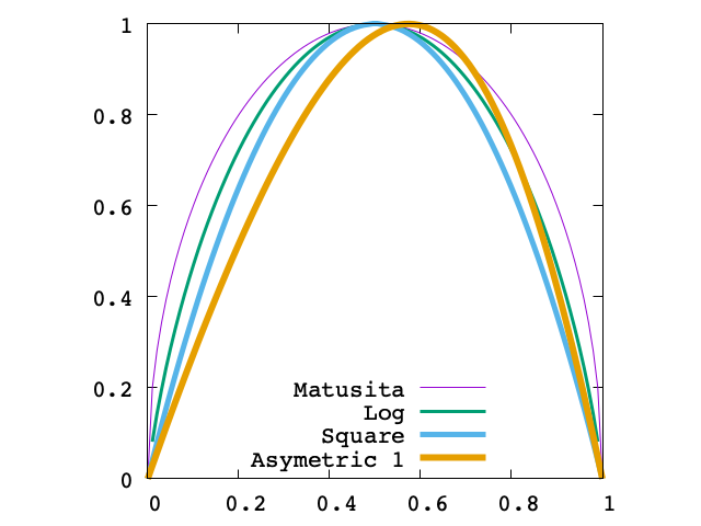
Conventional proper losses like the log-, square- or Matusita- are spd losses with L¯​(0)=L¯​(1)=ℓ1​(1)=ℓ−1​(0)=0\underline{L}(0)=\underline{L}(1)=\ell_{1}(1)=\ell_{-1}(0)=0. Losses satisfying ℓ1​(1)=ℓ−1​(0)=0\ell_{1}(1)=\ell_{-1}(0)=0 are called fair in [60].

Population loss

Usually in ML, we are given a training sample 𝒮=.{(𝒙i,yi),i=1,2,…,m}\mathcal{S}\stackrel{{\scriptstyle\mathrm{.}}}{{=}}\{(\bm{x}_{i},y_{i}),i=1,2,...,m\} where 𝒙i\bm{x}_{i} is an observation from a domain 𝒳\mathcal{X} and yi∈𝒴=.{0,1}y_{i}\in\mathcal{Y}\stackrel{{\scriptstyle\mathrm{.}}}{{=}}\{0,1\} a binary representation for classes in a two-classes problem (0 goes for the "negative class", 1 for the "positive class"). In the CPE setting, we wish to learn an estimated posterior η~:𝒳→[0,1]\tilde{\upeta}:\mathcal{X}\rightarrow[0,1], and to do so, following some of [40]’s notations, we wish to learn η~\tilde{\upeta} by minimizing a population loss called a risk:

Φ⁡(η~,𝒮)\displaystyle\Phi(\tilde{\upeta},\mathcal{S}) =.\displaystyle\stackrel{{\scriptstyle\mathrm{.}}}{{=}} 𝔼i∼[m]​[ℓ⁡(yi,η~​(𝒙i))].\displaystyle\mathbb{E}_{i\sim[m]}\left[\ell(y_{i},\tilde{\upeta}(\bm{x}_{i}))\right]. (4)

As already explained in the introduction, we assume training on the whole domain to fit in the framework of [40]’s negative results, so the question of the generalisation abilities of models does not arise. In such a case, Bayes rule can be computed from the training data.

3 Surrogate losses and a proper paradox

Link and canonical losses

The inverse link of a spd loss is:

η~​(z)\displaystyle\tilde{\upeta}(z) =.\displaystyle\stackrel{{\scriptstyle\mathrm{.}}}{{=}} (−L¯′)−1​(z).\displaystyle({{-\underline{L}}^{\prime}})^{-1}(z). (5)

One can check that for any spd loss, Im⁡(η~)=[0,1]\mathrm{Im}(\tilde{\upeta})=[0,1], and it turns out that the inverse link provides a maximum likelihood estimator of the posterior CPE given a learned real-valued predictor h:𝒳→ℝh:\mathcal{X}\rightarrow\mathbb{R} [54, Section 5]. A substantial part of ML learns naturally real-valued models (from linear models to deep nets) so the link is important to "naturally" embed the prediction in a CPE loss. A loss using its own link for the embedding is called a canonical loss [60]. One can use a different link, in which case the loss is called "composite" but technical conditions arise to keep the whole construction proper [60] so we restrict ourselves to the simplest case of proper canonical losses and call them proper for short. When used with real-valued prediction, spd losses have a remarkable analytical form – called in general a surrogate loss [54] (and references therein) – from which directly arises the apparent paradox we mentioned in the introduction.

Surrogate losses

It comes from e.g. [52, Theorem 1] that any spd loss can be written for a real valued classifier h:𝒳→ℝh:\mathcal{X}\rightarrow\mathbb{R} on example (𝒙,y)(\bm{x},y) with binary-described class y∈𝒴y\in\mathcal{Y} as:

ℓ⁡(y,h⁡(𝒙))\displaystyle\ell(y,h(\bm{x})) =\displaystyle= D−L¯(y∥−L¯′−1(h(𝒙)))\displaystyle D_{{-\underline{L}}}\left(y\|{{-\underline{L}}^{\prime}}^{-1}(h(\bm{x}))\right) (6) =.\displaystyle\stackrel{{\scriptstyle\mathrm{.}}}{{=}} −L¯​(y)+(−L¯)⋆​(h⁡(𝒙))−y​h​(𝒙)\displaystyle{-\underline{L}}(y)+{(-\underline{L})}^{\star}(h(\bm{x}))-yh(\bm{x}) =\displaystyle= −L¯​(y)+ϕℓ​(−h⁡(𝒙))−y​h​(𝒙)⏟model dependent term,\displaystyle{-\underline{L}}(y)+\underbrace{{\upphi_{\ell}}(-h(\bm{x}))-yh(\bm{x})}_{\mbox{model dependent term}}, with ϕℓ​(z)\displaystyle{\upphi_{\ell}}(z) =.\displaystyle\stackrel{{\scriptstyle\mathrm{.}}}{{=}} (−L¯)⋆​(−z).\displaystyle(-\underline{L})^{\star}(-z). (7)

We single out function ϕℓ{\upphi_{\ell}} to follow notations from [40] (we add ℓ\ell in index to remind it depends on the loss). Here, D−L¯D_{-\underline{L}} is a Bregman divergence with generator −L¯{-\underline{L}} (definition using the convex conjugate e.g. in [2]). Note that (6) does not fit to the classical margin loss definition in ML (as in, e.g., [40]), however, when the loss is in addition symmetric – which happens to be the case for most ML losses like log-, square-, Matusita, etc. –, the formula simplifies further to a margin loss formulation. Indeed, we remark L¯​(u)=L¯​(1−u){\underline{L}}(u)={\underline{L}}(1-u) and it comes (−L¯)⋆​(−z)=(−L¯)⋆​(z)−z{(-\underline{L})}^{\star}(-z)={(-\underline{L})}^{\star}(z)-z. Using a "dual" real-valued class y∗∈𝒴∗=.{−1,1}y^{*}\in\mathcal{Y}^{*}\stackrel{{\scriptstyle\mathrm{.}}}{{=}}\{-1,1\} (1 still goes to the positive class), we can rewrite the loss as

ℓ⁡(y∗,h⁡(𝒙))\displaystyle\ell(y^{*},h(\bm{x})) =\displaystyle= −L¯​(1+y∗2)+ϕℓ​(y∗​h​(𝒙))⏟model dependent term.\displaystyle{-\underline{L}}\left(\frac{1+y^{*}}{2}\right)+\underbrace{{\upphi_{\ell}}(y^{*}h(\bm{x}))}_{\mbox{model dependent term}}. (8)

At this stage, it is important to insist that the "loss", in the CPE framework, is ℓ\ell (1). Eq. (8) is a reparameterisation of it. The distinction is not superficial: the Bayes risk L¯\underline{L} in (3) is concave in its probability argument, while ϕℓ{\upphi_{\ell}} in (7) is convex in its real-valued argument. Popular choices for ℓ\ell, like log-, square-, Matusita, yield as popular forms for ϕℓ{\upphi_{\ell}}, respectively logistic, square and Matusita. They are often called losses as well since they quantify a discrepancy, but equally often they are called surrogates (or surrogate losses) for the simple reason that when properly scaled, they yield upperbounds of the "historic loss" of ML, the 0/1 loss [32], which with our notations equates ⟦sign(h(𝒙))≠y∗⟧\llbracket\mathrm{sign}(h(\bm{x}))\neq y^{*}\rrbracket.

For learning, we can focus only in the model dependent term in (6), (8) and thus define the population (surrogate) risk as:

Φ⁡(h,𝒮)\displaystyle\Phi(h,\mathcal{S}) =.\displaystyle\stackrel{{\scriptstyle\mathrm{.}}}{{=}} 𝔼i∼[m]​[ℓ⁡(yi∗,h⁡(𝒙i))]+𝔼i∼[m]​[L¯​(1+yi∗2)]\displaystyle\mathbb{E}_{i\sim[m]}\left[\ell(y_{i}^{*},h(\bm{x}_{i}))\right]+\mathbb{E}_{i\sim[m]}\left[{\underline{L}}\left(\frac{1+y_{i}^{*}}{2}\right)\right]
=\displaystyle= {𝔼i∼[m]​[ϕℓ​(−h⁡(𝒙i))−yi​h​(𝒙i)](general form)𝔼i∼[m]​[ϕℓ​(yi∗​h​(𝒙i))](for symmetric losses).\displaystyle\left\{\begin{array}[]{cl}\mathbb{E}_{i\sim[m]}\left[{\upphi_{\ell}}(-h(\bm{x}_{i}))-y_{i}h(\bm{x}_{i})\right]&\mbox{(general form)}\\ \mathbb{E}_{i\sim[m]}\left[{\upphi_{\ell}}(y_{i}^{*}h(\bm{x}_{i}))\right]&\mbox{(for symmetric losses)}\end{array}\right..

A Bayes born paradox

There is one technical argument that needs to be shown to relate the surrogate form in (3) to [40]’s results: we need to show that the corresponding surrogates of any symmetric spd loss fits to their blueprint margin loss.

Lemma 1.

For any spd loss, ϕℓ{\upphi_{\ell}} is C1C^{1}, convex, decreasing, has ϕℓ′​(0)<0{\upphi_{\ell}}^{\prime}(0)<0 and limz→+∞ϕℓ​(z)=L¯​(0)\lim_{z\rightarrow+\infty}{\upphi_{\ell}}(z)=\underline{L}(0).

Proof in Appendix, Section II.1. Hence, if we offset the constant L¯​(0)\underline{L}(0) or just assume it is 0, any symmetric (8) spd loss fits to [40, Definition 1].

We now explain [40, Section 4]’s data. The domain 𝒳=ℝ2\mathcal{X}=\mathbb{R}^{2} and we have a sample

𝒮clean\displaystyle\mathcal{S}_{\mbox{\tiny{clean}}} =.\displaystyle\stackrel{{\scriptstyle\mathrm{.}}}{{=}} {([10],1),([γ−γ],1),([γ−γ],1),([γK​γ],1)}.\displaystyle\left\{\left(\left[\begin{array}[]{c}1\\ 0\end{array}\right],1\right),\left(\left[\begin{array}[]{c}\gamma\\ -\gamma\end{array}\right],1\right),\left(\left[\begin{array}[]{c}\gamma\\ -\gamma\end{array}\right],1\right),\left(\left[\begin{array}[]{c}\gamma\\ K\gamma\end{array}\right],1\right)\right\}.

In [40], K=5K=5 and γ>0\gamma>0 is a margin parameter. Since all labels are positive, we easily get Bayes prediction, η⁡(𝒙)=1=ℙ⁡[𝖸=1|𝖷=𝒙]\upeta(\bm{x})=1=\mathbb{P}[\mathsf{Y}=1|\mathsf{X}=\bm{x}]. In the setting of [40], it is a simple matter to check that the optimal real-valued linear separator (𝖫𝖲{\mathsf{LS}}) hh minimizing Φ⁡(h,𝒮clean)\Phi(h,\mathcal{S}_{\mbox{\tiny{clean}}}) makes zero mistakes on predicting labels for 𝒮clean\mathcal{S}_{\mbox{\tiny{clean}}}. One would expect this to happen since the loss ℓ\ell at the core is proper, yet this seems to all go sideways as soon as label noise enters the picture. We replace 𝒮clean\mathcal{S}_{\mbox{\tiny{clean}}} by a noisy (multiset or bag) version 𝒮noisy\mathcal{S}_{\mbox{\tiny{noisy}}},

𝒮noisy\displaystyle\mathcal{S}_{\mbox{\tiny{noisy}}} =.\displaystyle\stackrel{{\scriptstyle\mathrm{.}}}{{=}} N​ copies of ​𝒮clean∪1​ copy of ​𝒮clean​with labels flipped.\displaystyle N\mbox{ copies of }\mathcal{S}_{\mbox{\tiny{clean}}}\cup 1\mbox{ copy of }\mathcal{S}_{\mbox{\tiny{clean}}}\mbox{with labels flipped}. (21)

This mimics a symmetric label noise level ηy=1/(N+1)\eta_{\mbox{\tiny{{y}}}}=1/(N+1), with N>1N>1 [40]. The paradox mentioned above comes from the following two observations: (i) Bayes posterior prediction with noise becomes η⁡(𝒙)=1−ηy>1/2\upeta(\bm{x})=1-\eta_{\mbox{\tiny{{y}}}}>1/2, which still makes no error on 𝒮clean\mathcal{S}_{\mbox{\tiny{clean}}}, and (ii) [40] show that regardless of this noise level, for any margin loss ϕℓ{\upphi_{\ell}} complying with Lemma 1, the optimal model is as bad as the fair coin on 𝒮clean\mathcal{S}_{\mbox{\tiny{clean}}}. Since symmetric spd losses (3) fit to Lemma 1, [40]’s optimal model should have the same properties as Bayes’ predictor, yet this clearly does not happen. The picture looks even gloomier as algorithms enter the stage: despite its acclaimed performances [23], boosting can perform so badly that after a single iteration its "strong" model hits the fair coin prediction. Not only do we hit a paradox from the standpoint of the optimal model, we also observe a stark failure of a powerful algorithmic machinery. There are clearly "things that break" in the trio (algorithm, loss, model) in the context of [40]. Post-[40] work clearly shed light on the algorithm and loss as the culprits (Section I).

In the context of properness, we have shown that the "margin form" parameterisation of the loss used by [40] is in fact not mandatory as asymmetric losses do not comply with it. Because asymmetry alleviates ties between partial losses, one could legitimately hope that it could address the paradox. We now show that it is not the case as [40]’s results mentioned above still stand without symmetry.

4 Long and Servedio’s results hold without symmetry

We reuse some of [40]’s notations and first denote BϕidealB_{\upphi}^{\mbox{{\tiny ideal}}} the algorithm returning the optimal linear separator (𝖫𝖲{\mathsf{LS}}) hh minimizing (3).

Lemma 2.

For any N>1N>1, there exists γ>0,K>0\gamma>0,K>0 such that when trained on 𝒮noisy\mathcal{S}_{\mbox{\tiny{noisy}}}, BϕidealB_{\upphi}^{\mbox{{\tiny ideal}}}’s classifier has at most 50%50\% accuracy on 𝒮clean\mathcal{S}_{\mbox{\tiny{clean}}}.

Proof in Appendix, Section II.2. The proof displays an interesting phenomenon for asymmetric losses, which is not observed on [40]’s results. If the noise ηy\eta_{\mbox{\tiny{{y}}}} is large enough and the asymmetry such that ϕℓ′​(0)<ηy−1{\upphi_{\ell}}^{\prime}(0)<\eta_{\mbox{\tiny{{y}}}}-1, then the optimal classifier can do more than 50%50\% mistakes on 𝒮clean\mathcal{S}_{\mbox{\tiny{clean}}} – thus perform worse than the unbiased coin. This cannot happen with symmetric losses since in this case ϕℓ′(0)=−1/2{\upphi_{\ell}}^{\prime}(0)=-1/2 and we constrain ηy<1/2\eta_{\mbox{\tiny{{y}}}}<1/2. What this shows is that asymmetry, while accomodating non-trivial different misclassification costs depending on the class, can lead to non-trivial pitfalls over noisy data.

Similarly to [40], we denote Bϕ,TearlyB_{\upphi,T}^{\mbox{{\tiny early}}} the booster of (3) which proceeds by following the boosting blueprint as described in [40]; we assume that the weak learner chooses the weak classifier offering the largest absolute edge (31), returning nil if all possible edges are zero (and then the booster stops). We let 𝒮clean,θ,𝒮noisy,θ\mathcal{S}_{\mbox{\tiny{clean}},\theta},\mathcal{S}_{\mbox{\tiny{noisy}},\theta} denote 𝒮clean,𝒮noisy\mathcal{S}_{\mbox{\tiny{clean}}},\mathcal{S}_{\mbox{\tiny{noisy}}} with observations rotated by an angle θ\theta.

Lemma 3.

For any N>1,T≥1N>1,T\geq 1, there exists γ>0,K>0,θ∈[0,2​π]\gamma>0,K>0,\theta\in[0,2\pi] such that when trained on 𝒮noisy,θ\mathcal{S}_{\mbox{\tiny{noisy}},\theta}, within at most TT boosting iterations Bϕ,TearlyB_{\upphi,T}^{\mbox{{\tiny early}}} hits a classifier at most 50%50\% accurate on 𝒮clean,θ\mathcal{S}_{\mbox{\tiny{clean}},\theta}.

Proof in Appendix, Section II.3.

5 The boosting blueprint does provide a fix

We investigate a new boosting algorithm learning model architectures that generalise those of decision trees and linear separators, among other model classes. We call such models partition-linear models (plm). The algorithm boosts any spd loss using the blueprint boosting algorithm of [40]. To our knowledge, it is the first boosting algorithm which can provably boost asymmetric proper losses, which is non trivial as it involves two different forms of the corresponding surrogate that are not compliant with the classical margin representation [40]. A simple way to define a plm HtH_{t} from a sequence of triples (αj,hj,𝒳j)j∈[t](\alpha_{j},h_{j},\mathcal{X}_{j})_{j\in[t]} (where αj∈ℝ,hj∈ℝ𝒳,𝒳j⊆𝒳\alpha_{j}\in\mathbb{R},h_{j}\in\mathbb{R}^{\mathcal{X}},\mathcal{X}_{j}\subseteq\mathcal{X}) is, for t≥1t\geq 1:

Ht​(𝒙)\displaystyle H_{t}(\bm{x}) =\displaystyle= {Ht−1​(𝒙)+αt​ht​(𝒙) if 𝒙∈𝒳tHt−1​(𝒙) otherwise,\displaystyle\left\{\begin{array}[]{ccl}H_{t-1}(\bm{x})+\alpha_{t}h_{t}(\bm{x})&\mbox{ if }&\bm{x}\in\mathcal{X}_{t}\\ H_{t-1}(\bm{x})&\lx@intercol\mbox{ otherwise}\hfil\lx@intercol\end{array}\right., (25)
=\displaystyle= ∑t=1T⟦𝒙∈𝒳t⟧⋅αtht(𝒙),\displaystyle\sum_{t=1}^{T}\llbracket\bm{x}\in\mathcal{X}_{t}\rrbracket\cdot\alpha_{t}h_{t}(\bm{x}),

and we add H0​(𝒙)=.0,∀𝒙∈𝒳H_{0}(\bm{x})\stackrel{{\scriptstyle\mathrm{.}}}{{=}}0,\forall\bm{x}\in\mathcal{X}22 2 We can equivalently consider that ht=0h_{t}=0 in 𝒳\𝒳t\mathcal{X}\backslash\mathcal{X}_{t}. We opt for (5) since it makes a clear distinction for 𝒳t\mathcal{X}_{t}. Notice that this setting generalizes boosting with weak hypotheses that abstain [66].. We also define the weight function

w⁡((𝒙,y),H)\displaystyle w((\bm{x},y),H) =.\displaystyle\stackrel{{\scriptstyle\mathrm{.}}}{{=}} y−y∗⋅(−L¯′)−1​(H⁡(𝒙)),\displaystyle y-y^{*}\cdot({-\underline{L}^{\prime}})^{-1}(H(\bm{x})), (26)

which is in [0,1][0,1]. Notice we use both (real and binary) class encodings in the weight function, recalling the relationship y∗=.2​y−1∈{−1,1}y^{*}\stackrel{{\scriptstyle\mathrm{.}}}{{=}}2y-1\in\{-1,1\}. Algorithm ModaBoost presents the boosting approach to learning plm. Note that ModaBoost picks the subset of 𝒮\mathcal{S} on which to evaluate this hypothesis, which corresponds e.g. in decision trees induction to the choice of a leaf to split via a call to the weak learner [33].

Algorithm 1 ModaBoost(𝒮,ℓ,wl,T)(\mathcal{S},\ell,\textsc{wl},T)
 Input: Dataset 𝒮={(𝒙i,yi)}i=1m\mathcal{S}=\{(\bm{x}_{i},y_{i})\}_{i=1}^{m}, spd loss ℓ\ell, weak learner wl, iteration number T≥1T\geq 1;
 Output: plm HTH_{T};
 Step 1 : ∀i∈[m],wi,1=.w⁡((𝒙i,yi),H0)\forall i\in[m],w_{i,1}\stackrel{{\scriptstyle\mathrm{.}}}{{=}}w((\bm{x}_{i},y_{i}),H_{0}) // weight initialisation
 Step 2 : for t=1,2,…,Tt=1,2,...,T
      Step 2.1 : pick 𝒳t⊆𝒳\mathcal{X}_{t}\subseteq\mathcal{X};
      Step 2.2 : ht←wl​(𝒘t∗,𝒮t)h_{t}\leftarrow\textsc{wl}(\bm{w}^{*}_{t},\mathcal{S}_{t});
          // weak learner call: 𝒮t=.{(𝒙i,yi)∈𝒮:𝒙i∈𝒳t}\mathcal{S}_{t}\stackrel{{\scriptstyle\mathrm{.}}}{{=}}\{(\bm{x}_{i},y_{i})\in\mathcal{S}:\bm{x}_{i}\in\mathcal{X}_{t}\}; 𝒘t∗=.𝒘t​ restricted to ​𝒮t\bm{w}^{*}_{t}\stackrel{{\scriptstyle\mathrm{.}}}{{=}}\bm{w}_{t}\mbox{ restricted to }\mathcal{S}_{t};
      Step 2.3 : compute αt\alpha_{t} as the solution to:
∑i∈[m]tw⁡((𝒙i,yi),Ht)⋅yi∗​ht​(𝒙i)\displaystyle\sum_{i\in[m]_{t}}w((\bm{x}_{i},y_{i}),H_{t})\cdot y_{i}^{*}h_{t}(\bm{x}_{i}) =\displaystyle= 0;\displaystyle 0; (27)
          // [m]t[m]_{t} = indices of 𝒮\mathcal{S} in 𝒮t\mathcal{S}_{t}; αt\alpha_{t} appears in HtH_{t}, see (5)
      Step 2.4 : ∀i∈[m]t,wt+1,i=.w⁡((𝒙i,yi),Ht)\forall i\in[m]_{t},w_{t+1,i}\stackrel{{\scriptstyle\mathrm{.}}}{{=}}w((\bm{x}_{i},y_{i}),H_{t})
          // weight update
 return HT​(𝒙)=.∑t=1T1𝒙∈𝒳t⋅αt​ht​(𝒙)H_{T}(\bm{x})\stackrel{{\scriptstyle\mathrm{.}}}{{=}}\sum_{t=1}^{T}\mathrm{1}_{\bm{x}\in\mathcal{X}_{t}}\cdot\alpha_{t}h_{t}(\bm{x});

Solutions to (27) are finite We assume without loss of generality that ±ht\pm h_{t} does not achieve 100%\% accuracy over 𝒮t\mathcal{S}_{t} (Step 2.2; otherwise there would be no need for boosting, at least in 𝒳t\mathcal{X}_{t}) and that max𝒮t⁡|ht|≪∞\max_{\mathcal{S}_{t}}|h_{t}|\ll\infty, "≪∞\ll\infty" denoting finiteness.

Lemma 4.

The solution to (27) satisfies |αt|≪∞|\alpha_{t}|\ll\infty.

Proof in Appendix, Section II.5.

The boosting abilities of ModaBoost

Given a real valued classifier HH and an example (𝒙,y∗)(\bm{x},y^{*}), we define the (unnormalized) edge or margin of HH on the example as y∗​H​(𝒙)y^{*}H(\bm{x}) [54, 65], a quantity that integrates both the accuracy of classification (its sign) and a confidence (its absolute value). Formal guarantees on edges / margins are not frequent in boosting [53, 65]. We now provide one such general guarantee for ModaBoost. While requirements on the weak hypotheses follow the weak learning assumption of boosting, the constraints on the loss itself are minimal: they essentially require it to be spd with partial losses meeting a lower-boundedness condition and a condition on derivatives.

Definition 5.1.

Let {ut}t∈ℕ\{u_{t}\}_{t\in\mathbb{N}} be a sequence of strictly positive reals. We say that the choice of 𝒳t\mathcal{X}_{t} in Step 2.1 of ModaBoost is "utu_{t} compliant" iff, letting J⁡(𝒲,t)=.Card⁡(𝒲)⋅(𝔼i∼𝒲​[wt,i])2J(\mathcal{W},t)\stackrel{{\scriptstyle\mathrm{.}}}{{=}}\mathrm{Card}(\mathcal{W})\cdot(\mathbb{E}_{i\sim\mathcal{W}}[w_{t,i}])^{2} where 𝒲⊆[m]\mathcal{W}\subseteq[m], Step 2.1 guarantees:

J⁡([m]t,t)\displaystyle J([m]_{t},t) ≥\displaystyle\geq ut⋅J⁡([m],t),∀t=1,2,…,\displaystyle u_{t}\cdot J([m],t),\forall t=1,2,..., (28)

Notice that the sum of terms ∑t=1Tut\sum_{t=1}^{T}u_{t} is strictly increasing and thus invertible. Let U:ℕ∗→ℝ+U:\mathbb{N}_{*}\rightarrow\mathbb{R}_{+} such that U⁡(T)=.∑t=1TutU(T)\stackrel{{\scriptstyle\mathrm{.}}}{{=}}\sum_{t=1}^{T}u_{t}. The role of JJ is fundamental in our results and can guide the choice of 𝒳t\mathcal{X}_{t} in Step 2.1: in short, the larger utu_{t}, the better the rates. Lemma 6 gives a concrete and intuitive simplification of JJ in the case of decision trees. In the most general case, it is good to keep in mind the intuition of boosting that the weight of an example is larger as the outcome of the current classifier gets worse. Hence, (28) encourages focus on 𝒳t\mathcal{X}_{t} with a large number of examples (Card⁡([m]t)\mathrm{Card}([m]_{t})) and with large weights (𝔼i∼[m]t​[wt,i]\mathbb{E}_{i\sim[m]_{t}}[w_{t,i}]) – hence with subpar current classification.

Theorem 1.

Suppose the following assumptions are satisfied on the loss and weak learner:

  • LOSS

    the loss is strictly proper differentiable; its partial losses are such that ∃κ>0,C∈ℝ\exists\kappa>0,C\in\mathbb{R},

    ℓ−1​(0),ℓ1​(1)\displaystyle\ell_{-1}(0),\ell_{1}(1) ≥\displaystyle\geq C,\displaystyle C, (29)
    inf{ℓ−1′−ℓ1′}\displaystyle\inf\{\ell_{-1}^{\prime}-\ell_{1}^{\prime}\} ≥\displaystyle\geq κ.\displaystyle\kappa. (30)
  • WLA

    There exists a constant γwl>0\upgamma_{\mbox{\tiny{{wl}}}}>0 such that at each iteration t∈[T]t\in[T], the weak hypothesis hth_{t} returned by wl satisfies33 3 The quantity in the absolute value is sometimes called the (normalized) edge of hth_{t}; it takes values in [−1,1][-1,1].

    |∑i∈[m]twt,i∑j∈[m]twt,j⋅yi∗⋅ht​(𝒙i)maxj∈[m]t⁡|ht​(𝒙j)||\displaystyle\left|\sum_{i\in[m]_{t}}\frac{w_{t,i}}{\sum_{j\in[m]_{t}}w_{t,j}}\cdot y^{*}_{i}\cdot\frac{h_{t}(\bm{x}_{i})}{\max_{j\in[m]_{t}}|h_{t}(\bm{x}_{j})|}\right| ≥\displaystyle\geq γwl.\displaystyle\upgamma_{\mbox{\tiny{{wl}}}}. (31)

Then for any θ≥0,ε>0\theta\geq 0,\varepsilon>0, letting w¯​(θ)=.min⁡{1−(−L¯′)−1​(θ),(−L¯′)−1​(−θ)}\underline{w}(\theta)\stackrel{{\scriptstyle\mathrm{.}}}{{=}}\min\{1-({-\underline{L}^{\prime}})^{-1}(\theta),({-\underline{L}^{\prime}})^{-1}(-\theta)\}, if ModaBoost is run for at least

T\displaystyle T ≥\displaystyle\geq U−1​(2​(Φ​(H0,𝒮)−C)κ⋅ε2​w¯​(θ)2​γwl2)\displaystyle U^{-1}\left(\frac{2\left(\Phi(H_{0},\mathcal{S})-C\right)}{\kappa\cdot\varepsilon^{2}\underline{w}(\theta)^{2}\upgamma_{\mbox{\tiny{{wl}}}}^{2}}\right) (32)

iterations, then we are guaranteed

ℙi∼[m][yi∗HT(𝒙i)≤θ]\displaystyle\mathbb{P}_{i\sim[m]}[y^{*}_{i}H_{T}(\bm{x}_{i})\leq\theta] <\displaystyle< ε.\displaystyle\varepsilon. (33)

Here, UU is built from a sequence of utu_{t} such that the choice of 𝒳t\mathcal{X}_{t} in Step 2.1 is utu_{t} compliant.

Proof in Appendix, Section II.6. The proof of the Theorem involves as intermediate step the proof that the surrogate Φ⁡(HT,𝒮)\Phi(H_{T},\mathcal{S}) is also boosted, which is of independent interest given [40]’s framework and the potential asymmetry of the loss (Theorem B in Appendix). Figure 1 depicts some key functions used in ModaBoost and Theorem 1.

Refer to caption
Figure 1: Schematic depiction of key functions used for weights (26) and Theorem 1 on an example of loss.
Remark 1.

The LOSS requirements are weak. It can be shown that strict properness implies inf{ℓ−1′−ℓ1′}>0\inf\{\ell_{-1}^{\prime}-\ell_{1}^{\prime}\}>0 [60, Theorem 1]; since the domain of the partial losses is closed, we are merely naming the strictly positive infimum with condition inf{ℓ−1′−ℓ1′}≥κ>0\inf\{\ell_{-1}^{\prime}-\ell_{1}^{\prime}\}\geq\kappa>0. The "extremal" value condition for partial losses (ℓ−1​(0),ℓ1​(1)≥C\ell_{-1}(0),\ell_{1}(1)\geq C) is also weak as if it did not hold, partial losses would not be lower-bounded on each’s respective best possible prediction, which would make little sense. Usually, C=0C=0 (the best predictions occur no loss) and such losses, that include many popular choices like square-, log-, Matusita, are called "fair" [60].

We now give five possible instantiations of ModaBoost, each with separate discussion about utu_{t} compliance and boosting rates. We start by the two most important ones (linear separators and decision trees), providing additional details for decision trees on how ModaBoost emulates well known algorithms.

Application of ModaBoost #​1\#1: linear separators (𝖫𝖲{\mathsf{LS}})

This is a trivial use of ModaBoost.

⊳\triangleright utu_{t} compliance and the weak learner: 𝒳t=𝒳,∀t\mathcal{X}_{t}=\mathcal{X},\forall t so we trivially have ut=1​(∀t)u_{t}=1(\forall t) compliance and the weak learner returns an index of a feature to leverage.

⊳\triangleright Boosting rate: we have the guarantee that ℙi∼[m][yi∗HT(𝒙i)≤θ]<ε\mathbb{P}_{i\sim[m]}[y^{*}_{i}H_{T}(\bm{x}_{i})\leq\theta]<\varepsilon if

T\displaystyle T ≥\displaystyle\geq 2​(Φ​(H0,𝒮)−C)κ⋅ε2​w¯​(θ)2​γwl2⏟=.B𝖫𝖲=O~​(1ε2​γwl2),\displaystyle\underbrace{\frac{2\left(\Phi(H_{0},\mathcal{S})-C\right)}{\kappa\cdot\varepsilon^{2}\underline{w}(\theta)^{2}\upgamma_{\mbox{\tiny{{wl}}}}^{2}}}_{\stackrel{{\scriptstyle\mathrm{.}}}{{=}}\mathrm{B}_{\mbox{\tiny${\mathsf{LS}}$}}}=\tilde{O}\left(\frac{1}{\varepsilon^{2}\upgamma_{\mbox{\tiny{{wl}}}}^{2}}\right), (34)

a dependence (the tilda removes dependences in other factors) that fits to the general optimal lower-bound in γwl\upgamma_{\mbox{\tiny{{wl}}}} [1] but is suboptimal in ε\varepsilon, albeit not far from the lowerbound of O⁡(1/ε)O(1/\varepsilon) [71]. Both the algorithm and its analysis generalises a previous one for linear separators and symmetric losses [54].

⊳\triangleright Effect of Long and Servedio’s data: Since ModaBoost falls in the negative result’s boosting blueprint of [40, Section 2.5], it does face the negative result of [40]. In fact, we can show a more impeding result directly in the setting of Lemma 2, i.e. without the rotation trick of Lemma 3, as with the square loss (which allows to compute quantities in closed form), ModaBoost hits a classifier as bad as the fair coin on 𝒮clean\mathcal{S}_{\mbox{\tiny{clean}}} in at most 2 iterations. This is shown and discussed in Appendix, Section II.4.

Application of ModaBoost #​2\#2: decision trees (𝖣𝖳{\mathsf{DT}})

This is a slightly more involved use of ModaBoost, from the "location" of the weak learner to the perhaps surprising observation that in this case, ModaBoost emulates and generalizes well known top-down induction schemes.

⊳\triangleright utu_{t} compliance and the weak learner: we investigate utu_{t} compliance from the general case where [m]t∈𝒫⁡([m])[m]_{t}\in\mathcal{P}([m]), where 𝒫⁡([m])\mathcal{P}([m]) is a partition of [m][m] in NtN_{t} subsets. Jensen’s inequality brings

∑𝒲∈𝒫⁡([m])J⁡(𝒲,t)\displaystyle\sum_{\mathcal{W}\in\mathcal{P}([m])}J(\mathcal{W},t) =\displaystyle= m⋅∑𝒲∈𝒫⁡([m])J⁡(𝒲,t)m\displaystyle m\cdot\sum_{\mathcal{W}\in\mathcal{P}([m])}\frac{J(\mathcal{W},t)}{m}
=\displaystyle= m⋅𝔼𝒲∼𝒫⁡([m])​(𝔼i∼𝒲​[wt,i])2\displaystyle m\cdot\mathbb{E}_{\mathcal{W}\sim\mathcal{P}([m])}\left(\mathbb{E}_{i\sim\mathcal{W}}[w_{t,i}]\right)^{2}
≥\displaystyle\geq m⋅(𝔼𝒲∼𝒫⁡([m])​[𝔼i∼𝒲​[wt,i]])2\displaystyle m\cdot\left(\mathbb{E}_{\mathcal{W}\sim\mathcal{P}([m])}\left[\mathbb{E}_{i\sim\mathcal{W}}[w_{t,i}]\right]\right)^{2}
=m⋅(𝔼i∼[m]​[wt,i])2=J⁡([m],t),\displaystyle=m\cdot\left(\mathbb{E}_{i\sim[m]}[w_{t,i}]\right)^{2}=J([m],t),

therefore there exists 𝒲∗∈𝒫⁡([m])\mathcal{W}^{*}\in\mathcal{P}([m]) such that J⁡(𝒲∗,t)≥(1/Nt)⋅J⁡([m],t)J(\mathcal{W}^{*},t)\geq(1/N_{t})\cdot J([m],t) and picking any such "heavy" subset of indices [m]t=𝒲∗[m]_{t}=\mathcal{W}^{*} guarantees utu_{t} compliance for ut=1/Ntu_{t}=1/N_{t}. Applied to a decision tree with tt leaves, we see that we can guarantee ut≥1/tu_{t}\geq 1/t, implying 𝒳t\mathcal{X}_{t} is the domain of a leaf of the current tree and the weak learner is used to find splits.

Regarding the weak learner, ModaBoost iteratively replaces a leaf in the current tree by a decision stump. There are two strategies for that: the first consists in asking the weak learner for one complete split, just like in [33], but ModaBoost would then fit a single correction (leveraging coefficient α.\alpha_{.}) for both leaves and this would be suboptimal. To correct every single leaf prediction separately, we let the weak learner return a split and a corresponding real-valued prediction for half the split, e.g. for "split_\_predicate = true". Quite remarkably, we show that if this meets the WLA, then so does the other half (for "split_\_predicate = false"). In other words, we get two WLA compliant weak hypotheses for the price of a single query to the weak learner, and both turn out to define the split sought. This is formalized in the following Lemma, which assumes wlog that the split variable is xix_{i}, continuous.

Lemma 5.

Suppose the weak learner returns 1xi≥a⋅ht\mathrm{1}_{x_{i}\geq a}\cdot h_{t} (ht∈ℝ∗h_{t}\in\mathbb{R}_{*} constant) that meets the WLA for the half split. Then the "companion" hypothesis ht′​(𝐱)=.1xi<a⋅(−ht)h^{\prime}_{t}(\bm{x})\stackrel{{\scriptstyle\mathrm{.}}}{{=}}\mathrm{1}_{x_{i}<a}\cdot(-h_{t}) satisfies the WLA.

Proof in Appendix, Section II.7. The choice of the leaf to split is simple: denote Λ⁡(H)\Lambda(H) the set of leaves of 𝖣𝖳{\mathsf{DT}} HH and λ\lambda a general leaf. Since the leaves of a 𝖣𝖳{\mathsf{DT}} induce a partition of the tree, we denote J⁡(λ)J(\lambda) the expression of J⁡(𝒲,t)J(\mathcal{W},t) for 𝒲={i:𝒙i​ reaches ​λ}\mathcal{W}=\{i:\bm{x}_{i}\mbox{ reaches }\lambda\}, omitting index tt for readability. Let us analyze what 𝒲∗\mathcal{W}^{*} would satisfy in this case.

Lemma 6.

We have

J⁡(λ)\displaystyle J(\lambda) ∝\displaystyle\propto pλ⋅(pλ+​(1−pλ+)⏟=L¯sq​(pλ+))2,\displaystyle p_{\lambda}\cdot(\underbrace{p^{+}_{\lambda}(1-p^{+}_{\lambda})}_{={\underline{L}^{\mbox{\tiny{{sq}}}}}(p^{+}_{\lambda})})^{2}, (35)

where pλ=.mλ/m,pλ+=.mλ+/mλp_{\lambda}\stackrel{{\scriptstyle\mathrm{.}}}{{=}}m_{\lambda}/m,p^{+}_{\lambda}\stackrel{{\scriptstyle\mathrm{.}}}{{=}}m^{+}_{\lambda}/m_{\lambda}, mλ=.Card⁡({i:𝐱i​ reaches ​λ}),mλ+=.Card⁡({i:𝐱i​ reaches ​λ∧yi=1})m_{\lambda}\stackrel{{\scriptstyle\mathrm{.}}}{{=}}\mathrm{Card}(\{i:\bm{x}_{i}\mbox{ reaches }\lambda\}),m^{+}_{\lambda}\stackrel{{\scriptstyle\mathrm{.}}}{{=}}\mathrm{Card}(\{i:\bm{x}_{i}\mbox{ reaches }\lambda\wedge y_{i}=1\}) and L¯sq​(u)=u⁡(1−u){\underline{L}^{\mbox{\tiny{{sq}}}}}(u)=u(1-u) is Bayes risk for the square loss.

Proof in Appendix, Section II.8. Hence, the leaf to split in Step 2.1 has a good compromise between its "weight" (pλp_{\lambda}) and its local error (since 2​pλ+​(1−pλ+)≥min⁡{pλ+,1−pλ+}2p^{+}_{\lambda}(1-p^{+}_{\lambda})\geq\min\{p^{+}_{\lambda},1-p^{+}_{\lambda}\}). In traditional "tree-based" boosting papers (from [33] to [55]), one usually picks the heaviest leaf (=arg⁡maxλ⁡pλ=\arg\max_{\lambda}p_{\lambda}) but it may well be a leaf with zero error – thus preventing boosting through splitting. Inversely, focusing only on large error to pick a leaf might point to leaves with too small weights to bring overall boosting compliance. Criterion J(.)J(.) strikes a balance weight vs error in the choice.
⊳\triangleright Boosting rate: We have ut≥1/tu_{t}\geq 1/t, with ∑t=1Tut≥∫0T𝑑z/(1+z)=log⁡(1+T)=.U⁡(T)\sum_{t=1}^{T}u_{t}\geq\int_{0}^{T}\mathrm{d}z/(1+z)=\log(1+T)\stackrel{{\scriptstyle\mathrm{.}}}{{=}}U(T), and so we are guaranteed that ℙi∼[m][yi∗HT(𝒙i)≤θ]<ε\mathbb{P}_{i\sim[m]}[y^{*}_{i}H_{T}(\bm{x}_{i})\leq\theta]<\varepsilon if

T\displaystyle T ≥\displaystyle\geq exp⁡(2​(Φ​(H0,𝒮)−C)κ⋅ε2​w¯​(θ)2​γwl2)⏟=.B𝖣𝖳=exp⁡(B𝖫𝖲)=exp⁡O~​(1ε2​γwl2)\displaystyle\underbrace{\exp\left(\frac{2\left(\Phi(H_{0},\mathcal{S})-C\right)}{\kappa\cdot\varepsilon^{2}\underline{w}(\theta)^{2}\upgamma_{\mbox{\tiny{{wl}}}}^{2}}\right)}_{\stackrel{{\scriptstyle\mathrm{.}}}{{=}}\mathrm{B}_{\mbox{\tiny${\mathsf{DT}}$}}}=\exp(\mathrm{B}_{\mbox{\tiny${\mathsf{LS}}$}})=\exp\tilde{O}\left(\frac{1}{\varepsilon^{2}\upgamma_{\mbox{\tiny{{wl}}}}^{2}}\right) (36)

(B𝖫𝖲\mathrm{B}_{\mbox{\tiny${\mathsf{LS}}$}} defined in (34)), which is comparable at θ=0\theta=0 to the bound of [33, Theorem 1] for CART and otherwise generalizes their results to margin/edge-based bounds.
⊳\triangleright Miscellaneous: we finish by a last analogy between ModaBoost and classical 𝖣𝖳{\mathsf{DT}} induction algorithms: there is a simple closed form solution for the leveraging coefficients α.\alpha_{.} that simplifies the loss.

Lemma 7.

Running ModaBoost to learn a decision tree HH gives

Φ⁡(H,𝒮)\displaystyle\Phi(H,\mathcal{S}) =\displaystyle= 𝔼λ∼Λ⁡(H)​[L¯​(pλ+)],\displaystyle\mathbb{E}_{\lambda\sim\Lambda(H)}\left[\underline{L}(p^{+}_{\lambda})\right], (37)

where we recall pλ+=.mλ+/mλp^{+}_{\lambda}\stackrel{{\scriptstyle\mathrm{.}}}{{=}}m^{+}_{\lambda}/m_{\lambda} and the weight of λ\lambda is mλ/mm_{\lambda}/m. Furthermore, the ModaBoost prediction computed at leaf λ\lambda, HλH_{\lambda}, is:

Hλ\displaystyle H_{\lambda} =\displaystyle= (−L¯′)​(pλ+).\displaystyle({-\underline{L}^{\prime}})\left(p^{+}_{\lambda}\right). (38)

Proof in Appendix, Section II.9. We conclude that running ModaBoost to learn a decision tree is largely equivalent to the minimisation of classical 𝖣𝖳{\mathsf{DT}} induction criteria [11, 59, 33, 55], and our boosting rate analysis generalizes those to asymmetric losses and edge / margin bounds. One can also finally notice that we can easily transform a 𝖣𝖳{\mathsf{DT}} learned using ModaBoost to a classical 𝖣𝖳{\mathsf{DT}} by "percolating" values down to the leaves, see Figure 2. such a connection between both types of models is not new as it dates back to [28] and was later exploited in various work (e.g. [42]).

Refer to caption Refer to caption Refer to caption
Figure 2: Left: 𝖣𝖳{\mathsf{DT}} learned using ModaBoost and its "classical" equivalent 𝖣𝖳{\mathsf{DT}}. Center: an equivalent representation using an alternating decision tree (black) and a more general 𝖠𝖣𝖳{\mathsf{ADT}} (black + red). Right: Using ModaBoost to learn a 𝖫𝖡𝖯{\mathsf{LBP}}: the main difference with 𝖣𝖳{\mathsf{DT}} is the current 𝒳t\mathcal{X}_{t} is the union of the domains of several leaves, yielding larger utu_{t}s and more efficient boosting.

⊳\triangleright Effect of Long and Servedio’s data: consider the more general setting where we have noise-free data with {0,1}\{0,1\} posterior values, and then labels are flipped independently with probability ηy<1/2\eta_{\mbox{\tiny{{y}}}}<1/2. The noisy proportion of positive examples at a leaf λ\lambda, p~λ+\tilde{p}_{\lambda}^{+}, satisfies p~λ+=ηy+(1−2​ηy)​pλ+\tilde{p}_{\lambda}^{+}=\eta_{\mbox{\tiny{{y}}}}+(1-2\eta_{\mbox{\tiny{{y}}}})p_{\lambda}^{+} (pλ+p_{\lambda}^{+} = noise-free proportion). Assume for simplicity we know the noise rate in advance (like in [30]) and do not have generalisation issues – we learn on the whole domain (like [30, Theorems 4, 6] or on the dataset of [40]). We say that the decision tree learned by ModaBoost with noise is not affected by noise if the sign of leaves would be the same as if they were computed without noise. In the context of Long and Servedio’s data, this implies 100%100\% accuracy on on the noise-free data.

Lemma 8.

If one of the two conditions is satisfied:

  • (S)

    the loss ℓ\ell is symmetric and ηy<1/2\eta_{\mbox{\tiny{{y}}}}<1/2, or

  • (A)

    the loss ℓ\ell is asymmetric, ηy<w¯​(0)\eta_{\mbox{\tiny{{y}}}}<\underline{w}(0) and leaves are split until (p∗=.(−L¯′)−1​(0)p^{*}\stackrel{{\scriptstyle\mathrm{.}}}{{=}}({-\underline{L}^{\prime}})^{-1}(0)):

    ∀λ∈Λ⁡(H),(pλ+≤min⁡{p∗−ηy1−2​ηy,12})∨(1−pλ+≤min⁡{(1−p∗)−ηy1−2​ηy,12}),\displaystyle\forall\lambda\in\Lambda(H),\left(p^{+}_{\lambda}\leq\min\left\{\frac{p^{*}-\eta_{\mbox{\tiny{{y}}}}}{1-2\eta_{\mbox{\tiny{{y}}}}},\frac{1}{2}\right\}\right)\vee\left(1-p^{+}_{\lambda}\leq\min\left\{\frac{(1-p^{*})-\eta_{\mbox{\tiny{{y}}}}}{1-2\eta_{\mbox{\tiny{{y}}}}},\frac{1}{2}\right\}\right), (39)

then the 𝖣𝖳{\mathsf{DT}} learned by ModaBoost is not affected by noise.

Proof in Appendix, Section II.10. We have left cases distinct for readability but in fact case (A) encompasses case (S), as this latter implies w¯​(0)=1/2=p∗\underline{w}(0)=1/2=p^{*}, making (39) always true. If we denote E⁡(H)\mathrm{E}(H) the error of the tree HH learned by ModaBoost without noise and E~​(H)\tilde{\mathrm{E}}(H) its error over noisified data, then we obtain from (S) that at any stage of the induction,

E~​(H)\displaystyle\tilde{\mathrm{E}}(H) =\displaystyle= ηy+(1−2​ηy)​E​(H),\displaystyle\eta_{\mbox{\tiny{{y}}}}+(1-2\eta_{\mbox{\tiny{{y}}}})\mathrm{E}(H), (40)

which is optimal [30, Section 5]. It is not hard to mirror the "extreme" negative result of Lemma I for 𝖫𝖲{\mathsf{LS}} into an extreme positive result for 𝖣𝖳{\mathsf{DT}} on [40]’s data: one easily obtains (from Lemma 7) that the root prediction of a 𝖣𝖳{\mathsf{DT}}, after leveraging in Step 2.3 of ModaBoost , is equal to Bayes posterior (which is constant over the whole domain). Hence, ModaBoost converges to Bayes prediction in a single iteration, which is confirmed experimentally (Section 6).

Application of ModaBoost #​3\#3: alternating decision trees (𝖠𝖣𝖳{\mathsf{ADT}})

Alternating decision trees were introduced in [22]. An 𝖠𝖣𝖳{\mathsf{ADT}} roughly consists of a root constant prediction and a series of stumps branching from their leaf prediction nodes in a tree graph, see Figure 2. The equivalent 𝖠𝖣𝖳{\mathsf{ADT}} representation of a 𝖣𝖳{\mathsf{DT}} would have outgoing degree 1 for all these stumps’ leaves. A general 𝖠𝖣𝖳{\mathsf{ADT}} makes this outdegree variable and a prediction is just the sum of the prediction along all paths an observation can follow from the 𝖠𝖣𝖳{\mathsf{ADT}}’s root node. If a stumps’ leaf branches on NN stumps, then we sum the NN corresponding predictions (and not just 1 for a 𝖣𝖳{\mathsf{DT}}). While using such models is interesting in terms of model’s parameterisation, one also sees advantages in terms of boosting, since summing boosted predictions (34) is more efficient than branching on boosted predictions (36), but the paper of [22] contains no such rate (note that the loss optimized here is AdaBoost’s exponential loss, which is not proper canonical).

⊳\triangleright utu_{t} compliance and the weak learner: these are just combinations of those for 𝖫𝖲{\mathsf{LS}} (when increasing a stump’s leaf outgoing degree with a new stump) and 𝖣𝖳{\mathsf{DT}} (when finding the test of a stump). Denote NN-𝖠𝖣𝖳{\mathsf{ADT}} the set of 𝖠𝖣𝖳{\mathsf{ADT}}s where non-leaf prediction nodes’ outdegree is fixed to be NN (inclusive of the root node). Notice that we can then boost while guaranteeing that ut=1u_{t}=1 for NN boosting iterations (at the root), then ut≥1/2u_{t}\geq 1/2 for NN boosting iterations and so on until the last NN iterations with ut≥N/Tu_{t}\geq N/T.

⊳\triangleright Boosting rate: assuming wlog TT a multiple of NN, we have thus ∑t=1Tut≥N⋅∑t=1T/N1/t≥N⋅∫0T/N𝑑z/(1+z)=N⋅log⁡(1+(T/N))=.U⁡(T)\sum_{t=1}^{T}u_{t}\geq N\cdot\sum_{t=1}^{T/N}1/t\geq N\cdot\int_{0}^{T/N}\mathrm{d}z/(1+z)=N\cdot\log(1+(T/N))\stackrel{{\scriptstyle\mathrm{.}}}{{=}}U(T), and so we are guaranteed that ℙi∼[m][yi∗HT(𝒙i)≤θ]<ε\mathbb{P}_{i\sim[m]}[y^{*}_{i}H_{T}(\bm{x}_{i})\leq\theta]<\varepsilon if

T\displaystyle T ≥\displaystyle\geq N⋅exp⁡(2​(Φ​(H0,𝒮)−C)N​κ⋅ε2​w¯​(θ)2​γwl2)⏟=.B𝖠𝖣𝖳=N​exp⁡(B𝖫𝖲N)=N​exp⁡O~​(1N​ε2​γwl2).\displaystyle\underbrace{N\cdot\exp\left(\frac{2\left(\Phi(H_{0},\mathcal{S})-C\right)}{N\kappa\cdot\varepsilon^{2}\underline{w}(\theta)^{2}\upgamma_{\mbox{\tiny{{wl}}}}^{2}}\right)}_{\stackrel{{\scriptstyle\mathrm{.}}}{{=}}\mathrm{B}_{\mbox{\tiny${\mathsf{ADT}}$}}}=N\exp\left(\frac{\mathrm{B}_{\mbox{\tiny${\mathsf{LS}}$}}}{N}\right)=N\exp\tilde{O}\left(\frac{1}{N\varepsilon^{2}\upgamma_{\mbox{\tiny{{wl}}}}^{2}}\right). (41)

This rate is really meaningful only when N≤B𝖫𝖲N\leq\mathrm{B}_{\mbox{\tiny${\mathsf{LS}}$}} since otherwise the 𝖠𝖣𝖳{\mathsf{ADT}} would meet (33) from the linear combinations of stumps branched at the root already. Bearing in mind that B𝖣𝖳,B𝖠𝖣𝖳\mathrm{B}_{\mbox{\tiny${\mathsf{DT}}$}},\mathrm{B}_{\mbox{\tiny${\mathsf{ADT}}$}} are non-tight lowerbounds, in such a regime, it is easy to see that an 𝖠𝖣𝖳{\mathsf{ADT}} can be exponentially more efficient than a 𝖣𝖳{\mathsf{DT}}, boosting-wise: for example, letting N=B𝖫𝖲N=\sqrt{\mathrm{B}_{\mbox{\tiny${\mathsf{LS}}$}}}, we obtain B𝖠𝖣𝖳≤exp⁡(−M​B𝖫𝖲)⋅B𝖣𝖳\mathrm{B}_{\mbox{\tiny${\mathsf{ADT}}$}}\leq\exp(-M\sqrt{\mathrm{B}_{\mbox{\tiny${\mathsf{LS}}$}}})\cdot\mathrm{B}_{\mbox{\tiny${\mathsf{DT}}$}} for some constant M>0M>0.

⊳\triangleright Effect of Long and Servedio’s data: since learning a 𝖣𝖳{\mathsf{DT}} achieves Bayes optimal prediction with a single root 𝖣𝖳{\mathsf{DT}}, the same happens for a single root 𝖠𝖣𝖳{\mathsf{ADT}}, and we get that the 𝖠𝖣𝖳{\mathsf{ADT}} learned by ModaBoost is not affected by noise.

Application of ModaBoost #​4\#4: (leveraged) nearest neighbors (𝖭𝖭{\mathsf{NN}})

nearest neighbor classification is one of the oldest supervised learning techniques [18]. Since we consider real-valued prediction, we implement 𝖭𝖭{\mathsf{NN}} classification by summing a real constant prediction at one observation’s neighbors and assume that tie neighbors are included in the voting sample (so one observation can end up with more than KK neighbors). Local predictions can have varying magnitudes, which represents a generalisation of nearest neighbor classification where magnitude is constant, but we still call such classifiers nearest neighbors, omitting the "leveraging" part.

⊳\triangleright utu_{t} compliance and the weak learner: the weak learner returns an example to leverage and thus 𝒳t\mathcal{X}_{t} is its reciprocal neighborhood (the set of examples for which it belongs to the KK-𝖭𝖭{\mathsf{NN}}). We assume wlog there are no "outliers" for classification, so the minimum size of this neighborhood is some Krec>0K_{\mbox{\tiny rec}}>0, yielding ut=Krec/m,∀tu_{t}=K_{\mbox{\tiny rec}}/m,\forall t.

⊳\triangleright Boosting rate: we immediately get ℙi∼[m][yi∗HT(𝒙i)≤θ]<ε\mathbb{P}_{i\sim[m]}[y^{*}_{i}H_{T}(\bm{x}_{i})\leq\theta]<\varepsilon if

T\displaystyle T ≥\displaystyle\geq 2​m​(Φ⁡(H0,𝒮)−C)Krec​κ⋅ε2​w¯​(θ)2​γwl2⏟=.B𝖭𝖭=m​B𝖫𝖲Krec=O~​(mKrec​ε2​γwl2),\displaystyle\underbrace{\frac{2m\left(\Phi(H_{0},\mathcal{S})-C\right)}{K_{\mbox{\tiny rec}}\kappa\cdot\varepsilon^{2}\underline{w}(\theta)^{2}\upgamma_{\mbox{\tiny{{wl}}}}^{2}}}_{\stackrel{{\scriptstyle\mathrm{.}}}{{=}}\mathrm{B}_{\mbox{\tiny${\mathsf{NN}}$}}}=\frac{m\mathrm{B}_{\mbox{\tiny${\mathsf{LS}}$}}}{K_{\mbox{\tiny rec}}}=\tilde{O}\left(\frac{m}{K_{\mbox{\tiny rec}}\varepsilon^{2}\upgamma_{\mbox{\tiny{{wl}}}}^{2}}\right), (42)

a bound substantially better and more general than the one of [51, Theorem 4], which was established for θ=0\theta=0 (namely, our assumptions are weaker, our result cover asymmetric losses and the dependency of (42) in KrecK_{\mbox{\tiny rec}} is better). It is important to remind at this point that this result is relevant to training and the margin bound holds over the training sample.

⊳\triangleright Effect of Long and Servedio’s data: it is not hard to see that the problem is equivalent to leveraging a constant prediction using all examples with a specific observation and the leveraging coefficient is the same as for a cdt where the root node’s support is restricted to the given observation, yielding optimal leveraging (after leveraging, each example’s new prediction is Bayes optimum) and so the 𝖭𝖭{\mathsf{NN}} leveraging learned by ModaBoost is not affected by noise. This applies for any choice of K≥1K\geq 1 neighbors for 𝖭𝖭{\mathsf{NN}}.

Application of ModaBoost #​5\#5: labeled branching programs (𝖫𝖡𝖯{\mathsf{LBP}})

A labeled branching program is a branching program with prediction values at each node, just like our encoding of 𝖣𝖳{\mathsf{DT}}, with the same way of classifying an observation – sum an observation’s path values from the root to a leaf. The key difference with classical branching programs is that to one leaf can correspond as many possible predictions as there are paths leading to it. See Figure 2 for an example.

⊳\triangleright utu_{t} compliance and the weak learner: the weak learner is the same as for 𝖣𝖳{\mathsf{DT}}, except it looks for a split over the union of a set of leaves in the current 𝖫𝖡𝖯{\mathsf{LBP}}, with the constraint that this split has to cut every leaf’s domain in two (this requirement can be removed if the user is comfortable that some inner nodes in the 𝖫𝖡𝖯{\mathsf{LBP}} may have out-degree 1). After the split is found, it is carried at each node and the outgoing arcs get to two new leaves only by merging the leaves of the stumps accordingly (call this procedure the split-merge process), as displayed in Figure 2. This makes the weak learner have the same properties as for 𝖣𝖳{\mathsf{DT}}, but of course, yields larger utu_{t} compliance than for 𝖣𝖳{\mathsf{DT}}, and so bring better boosting rates as we now show.

⊳\triangleright Boosting rate: suppose we run ModaBoost as for 𝖣𝖳{\mathsf{DT}} and start to merge nodes to always ensure ut≥βu_{t}\geq\upbeta for some β>1/T\upbeta>1/T. We get ∑t=1Tut≥∑t=1⌊1/β⌋(1/t)+β⁡(T−⌊1/β⌋)≥log⁡(1+⌊1/β⌋)+β​T−1≥log⁡(1/β)+β​T−1\sum_{t=1}^{T}u_{t}\geq\sum_{t=1}^{\lfloor 1/\upbeta\rfloor}(1/t)+\upbeta(T-\lfloor 1/\upbeta\rfloor)\geq\log(1+\lfloor 1/\upbeta\rfloor)+\upbeta T-1\geq\log(1/\upbeta)+\upbeta T-1. The choice β=T−c\upbeta=T^{-c} for a constant c∈(0,1)c\in(0,1) immediately leads that ℙi∼[m][yi∗HT(𝒙i)≤θ]<ε\mathbb{P}_{i\sim[m]}[y^{*}_{i}H_{T}(\bm{x}_{i})\leq\theta]<\varepsilon if

T\displaystyle T ≥\displaystyle\geq (2​(Φ​(H0,𝒮)−C)κ⋅ε2​w¯​(θ)2​γwl2)11−c⏟=.B𝖫𝖡𝖯=(B𝖫𝖲)11−c=O~​(1ε21−c​γwl21−c),\displaystyle\underbrace{\left(\frac{2\left(\Phi(H_{0},\mathcal{S})-C\right)}{\kappa\cdot\varepsilon^{2}\underline{w}(\theta)^{2}\upgamma_{\mbox{\tiny{{wl}}}}^{2}}\right)^{\frac{1}{1-c}}}_{\stackrel{{\scriptstyle\mathrm{.}}}{{=}}\mathrm{B}_{\mbox{\tiny${\mathsf{LBP}}$}}}=\left(\mathrm{B}_{\mbox{\tiny${\mathsf{LS}}$}}\right)^{\frac{1}{1-c}}=\tilde{O}\left(\frac{1}{\varepsilon^{\frac{2}{1-c}}\upgamma_{\mbox{\tiny{{wl}}}}^{\frac{2}{1-c}}}\right), (43)

a bound which is exponentially better than (36) for 𝖣𝖳{\mathsf{DT}}. While it does extend previous boosting rates to margins / edges [30, 43], (43) is suboptimal compared to the O~​(log2⁡(1/ε))\tilde{O}(\log^{2}(1/\varepsilon)) dependence of [43] shown for θ=0\theta=0.

⊳\triangleright Effect of Long and Servedio’s data: since learning a 𝖣𝖳{\mathsf{DT}} achieves Bayes optimal prediction with a single root 𝖣𝖳{\mathsf{DT}}, the same happens for a single root 𝖫𝖡𝖯{\mathsf{LBP}}, and we get that the 𝖫𝖡𝖯{\mathsf{LBP}} learned by ModaBoost is not affected by noise.

6 Toy experiments

We have implemented ModaBoost and performed toy experiments it in the framework of Long and Servedio [40], specifically train on 𝒮noisy\mathcal{S}_{\mbox{\tiny{noisy}}} and compute, as a function of γ\gamma in (3) (i) the number of iterations of ModaBoost until convergence, (ii) the accuracy on 𝒮clean\mathcal{S}_{\mbox{\tiny{clean}}} of the final classifier and (iii) the expected posterior of the classifier’s prediction compared to Bayes’. (i) is equivalent to the number of calls to wl until the weak learning assumption "breaks", i.e. until all possible weak hypotheses fail to meet (31) for some γwl=0.001\upgamma_{\mbox{\tiny{{wl}}}}=0.001. We test three model classes that ModaBoost is able to boost, 𝖫𝖲{\mathsf{LS}}, 𝖣𝖳{\mathsf{DT}} and 𝖭𝖭{\mathsf{NN}} (with K=1K=1), and consider four different proper loss functions in ModaBoost, three of which are symmetric and mainstream in ML (Matusita, log, square) and a fourth one, asymmetric, that we have engineered for the occasion. All details about those losses are in Appendix, Table 6.

We have crammed the results in Table 1 to get the overall picture. Results are otherwise presented in split format in Appendix, Tables A2, A3, A4. As predicted by theory, there is a stark contrast between 𝖫𝖲{\mathsf{LS}} on one hand and 𝖣𝖳{\mathsf{DT}} and 𝖭𝖭{\mathsf{NN}} on the other hand: while 𝖣𝖳{\mathsf{DT}} and 𝖭𝖭{\mathsf{NN}} consistently achieve Bayes prediction and thus are not affected by noise, 𝖫𝖲{\mathsf{LS}} learned always have very substantial degradation in their estimated posterior below a threshold γ\gamma, which translates to classifiers as accurate as the unbiased coin on 𝒮clean\mathcal{S}_{\mbox{\tiny{clean}}}. Remarkably, the number of iterations until the weak learner is "exhausted" of options meeting (31) for γwl=0.001\upgamma_{\mbox{\tiny{{wl}}}}=0.001 is very low: it takes just a few iterations for ModaBoost to be stuck with a bad 𝖫𝖲{\mathsf{LS}}, confirming a remark of Schapire [64] (See Appendix, Section I). Notably, the use of an asymmetric proper loss does not break any of these patterns. There are interesting differences appearing among choices for the noise parameter ηy\eta_{\mbox{\tiny{{y}}}}: increasing it tends to increase the threshold for phase transition in accuracy with 𝖫𝖲{\mathsf{LS}} and tends to reduce the number of calls to wl in this region for the square loss and our asymmetric loss. This last observation makes sense because increasing noise reduces the absolute edge of the weak classifiers. We also note that the result on 𝖭𝖭{\mathsf{NN}} for the number of iterations until wl is "exhausted" displays that the dependency in mm in (42)’s rate is pessimistic as it should depend on the number of distinct observations (=3 in [40]’s domain) rather than mm.

Accuracy on 𝒮clean\mathcal{S}_{\mbox{\tiny{clean}}} Expected posterior #\# Calls to wl
𝖫𝖲{\mathsf{LS}} 𝖣𝖳{\mathsf{DT}} 1-𝖭𝖭{\mathsf{NN}} 𝖫𝖲{\mathsf{LS}} 𝖣𝖳{\mathsf{DT}} 1-𝖭𝖭{\mathsf{NN}} 𝖫𝖲{\mathsf{LS}} 𝖣𝖳{\mathsf{DT}} 1-𝖭𝖭{\mathsf{NN}}

Matusita loss

[Uncaptioned image] [Uncaptioned image] [Uncaptioned image] [Uncaptioned image] [Uncaptioned image] [Uncaptioned image] [Uncaptioned image] [Uncaptioned image] [Uncaptioned image]

Log loss

[Uncaptioned image] [Uncaptioned image] [Uncaptioned image] [Uncaptioned image] [Uncaptioned image] [Uncaptioned image] [Uncaptioned image] [Uncaptioned image] [Uncaptioned image]

Square loss

[Uncaptioned image] [Uncaptioned image] [Uncaptioned image] [Uncaptioned image] [Uncaptioned image] [Uncaptioned image] [Uncaptioned image] [Uncaptioned image] [Uncaptioned image]

Asymmetric loss 1

[Uncaptioned image] [Uncaptioned image] [Uncaptioned image] [Uncaptioned image] [Uncaptioned image] [Uncaptioned image] [Uncaptioned image] [Uncaptioned image] [Uncaptioned image]
Table 1: Comparison of ModaBoost’s results with the induction of linear separators (𝖫𝖲{\mathsf{LS}}), decision trees (𝖣𝖳{\mathsf{DT}}) and 1-nearest neighbor (𝖭𝖭{\mathsf{NN}}) after training on 𝒮noisy\mathcal{S}_{\mbox{\tiny{noisy}}}; each plot has parameter γ\gamma in abscissa (3) and in ordinate respectively the accuracy on 𝒮noisy\mathcal{S}_{\mbox{\tiny{noisy}}} (left pane), the expected posterior estimation from 𝒮noisy\mathcal{S}_{\mbox{\tiny{noisy}}} (5) (Bayes’ optimum indicated in green rectangles, center pane), the number of iterations until the weak learner is "exhausted" (does not find a weak classifier with advantage γwl≥0.001\upgamma_{\mbox{\tiny{{wl}}}}\geq 0.001, right pane). Different curves correspond to different values of the noise parameter ηy\eta_{\mbox{\tiny{{y}}}}.

7 Discussion and conclusion: on parameterisation

A partial explanation for the confusion about the results of [40] can be offered via the notion of parametrisation. We elaborate this in terms of the three key ingredients of losses, models and algorithms. (We omit discussion of the other central ingredient of any learning problem, namely the data, or its theoretical representation as statistical experiments, which too, can be thought of parametrically [72].) Much ML research seems blind to the difference between a change of object, and a change in the parametrisation of an object. The clearest example of this is with loss functions, where it is known [75] that the features of a loss function that govern its mixability depend only upon the induced geometry of its superprediction set. (Mixability controls whether one attains fast or slow learning in the online worst-case sequence prediction setting [78]; there are generalisations of the notion that apply to the batch statistical setting [74]). From this perspective, losses are better thought of, and analysed in terms of the sets that they induce [19]. The commonplace desire that the loss function be convex (as a function) is controllable, independently, via a link function [60, 83]. Mathematically, the introduction of the link is tantamount to an (invertible, smooth) reparametrisation of the loss.

There is one other point to be made about the loss function. The abstract idea of a loss function was developed by Wald [80] as a formalisation of the notion that when solving a data-driven problem, one ultimately has some goal in mind, and that can be captured by an outcome-contingent utility [7], or ‘loss’. Thus the loss is part of the problem statement. In contrast, in the ML literature, such as that arising from [40], a loss function is considered as part of the specification of a ‘learning algorithm’ (means of solving the problem). From Wald’s perspective, all of the work inspired by [40] is a perhaps not so surprising side-effect of attempting to solve one problem (classification using 0-1 loss) by using a method that utilises a different loss. If one tries to repeat the negative example of [40] without the use of a surrogate, and always in terms of the Bayes optimal, there is nothing to see. When one adds some noise, the Bayes risk may change, but one will not see the apparent paradoxes of [40]. Recently, there has been a burst of research around new loss functions whole formulation aims to reduce the difficulty of the learning task, some becoming overwhelmingly popular [36]. One can see benefits of such a substantial shift from the normative view (of properness) to a more user-centric "à-la-Wald” design, but it usually comes with overloading loss functions with new hyperparameters. Technically, quantifing properties of the minimizers — in effect, answering the question "what can be learned from this loss" — can be non-trivial [69] but it is an important task: Long and Servedio’s result brightly demonstrates that we cannot reasonably stick with the choice "classifier = linear" and "loss = convex" (and eventually "algorithm = boosting") if the data is subject to corruption. One would have many reasons to stick with linear separators e.g. for their simplicity and interpretability. In such a case, changing the loss, breaking properness and eventually convexity might just be a requirement.

A less widespread example is the reparametrisation of a model class. It is known (starting with Vapnik and a long line of refinements in the ML literature) that the statistical complexity of a learning problem in the statistical batch setting is controlled by the complexity of the model class. This complexity is in terms of the class considered as a set, and is not influenced by how the elements of the class are parametrised. (The hardness is additionally influenced by the loss function, as per the above paragraph, however this is rarely made explicit; confer [74]). Thus the statistical complexity of learning with a model class comprising rational functions of degree nn will not depend upon whether the functions are parametrised in factored form, as partial fractions, or as ratios of polynomials in canonical sum form. Lest it be objected that no-one would use such a strange class, we note that in the simplest case analysable, classical sigmoidal neural networks can be reparametrised in terms of rational functions, and thus at least these three parametrisations are open to use [82]. The parametrisation, whilst not changing the model class (or, say its VC dimension) will change the behaviour of learning algorithms, in particular gradient based algorithms, which can misbehave due to attractors at infinity [8] — a phenomenon caused by the choice of parametrisation.

The final ingredient to consider is the algorithm. We have demonstrated that a boosting algorithm can be constructed that works successfully in the noisy situation (when using suitable model classes), but we have not really addressed head-on the perhaps more direct response to [40], which is to challenge the definition of what is, and what is not, a ‘boosting algorithm.’ There are several obvious ways to proceed here (e.g. in terms of what the boosting algorithm is provided as input, in the form of weak learners). But all such attempts stumble over a more challenging issue: namely that there is no sensible way to compare algorithms — we cannot even say ‘when is one algorithm equal to another?’ [10]. The irony is that the object that is most valorised in machine learning research, namely the algorithm, hardly satisfies the conceptual properties one demands of any ‘object’ — namely that we can tell when two objects are the same or different. We do not attempt to resolve this challenge here; indeed we think it is intrinsically unresolvable except up to a family of canonical isomorphisms, which need to be made explicit to really qualify as a legitimate answer [44] – perhaps this will give some insight into ‘natural’ parametrisations of different learning algorithms. Of course, instead of attempting to do this, we could just focus our attention on other perspectives!

One promising perspective, from the algorithmic standpoint is, we believe, the need for boosting algorithms for more complex / overparameterized architectures. Quite remarkably, in the dozens of references citing [40] we compile in Appendix, only one alludes to the key sufficient condition to solve [40]’s problem: Schapire mentions the potential lack of "richness" of hypotheses available to the weak learner in the context of AdaBoost [64]. This resonates with a comment precisely in [40] whereby linear separators lack capacity to control confidences as would richer classes do, a model’s flaw exploited by the negative results. Richness can be related to the choice in the weak hypotheses’ architecture and thus their model’s parameterisation; also, in the context of boosting, if we stick to the idea that the weak learner ultimately manipulates simple hypotheses – which is important e.g. in the context of 𝖣𝖳{\mathsf{DT}} where this entails a substantial combinatorial search of splits –, then the question of where to put the weak learning assumption arises. ModaBoost shows that we can consider that boosting a linear combination of models with the logistic loss, each of which is a top-down 𝖣𝖳{\mathsf{DT}} learned by minimizing C4.5’s binary entropy, is in fact a recursive application of ModaBoost with the same loss (log-loss) but different architectures, where the weak learning assumption only needs to be carried out at the tree’s splits, then used to learn trees with ModaBoost, then used to learn the linear combination of trees also with ModaBoost. Hence, complex architectures could then be learned using recursive calls to boosters like ModaBoost, progressively building the architecture from basic building blocks at the bottom of the recursion searchable by a weak learner. This is convenient but still far from the "architecture’s swiss army knife" optimization tool for ML that is stochastic gradient descent: can we make boosting "à-la-Kearns" [31] work for more architectures ?

To conclude, in this paper, we have used the founding theory of losses for class probability estimation (properness) and a new boosting algorithm to demonstrate that the source of the negative result in the context of Long and Servedio’s results is the model class. More than shining a new light on the model class’ "responsibility" for the negative result, we believe our results rather show pitfalls of general parameterisations of a ML problem, including model class but also the learning algorithm and the loss function it optimizes. It remains an open question as to whether such stark "breakdowns" can be shown for highly ML-relevant triples (algorithm, loss, model) different from ours / [40].

Acknowledgments

Many thanks to Phil Long for stimulating discussions around the material presented and tipping us on the rotation argument for the proof of Lemma 3.

References

  • [1] N. Alon, A. Gonen, E. Hazan, and S. Moran. Boosting simple learners. In STOC’21, 2021.
  • [2] S.-I. Amari and H. Nagaoka. Methods of Information Geometry. Oxford University Press, 2000.
  • [3] E. Amid, M.-K. Warmuth, R. Anil, and T. Koren. Robust bi-tempered logistic loss based on bregman divergences. In NeurIPS*32, pages 14987–14996, 2019.
  • [4] E. Amid, M.-K. Warmuth, and S. Srinivasan. Two-temperature logistic regression based on the Tsallis divergence. In 22nd AISTATS, volume 89, pages 2388–2396, 2019.
  • [5] H. Bao, C. Scott, and M. Sugiyama. Calibrated surrogate losses for adversarially robust classification. In 33r​d{}^{~rd} COLT, volume 125, pages 408–451, 2020.
  • [6] S. Ben-David, D. Loker, N. Srebro, and K. Sridharan. Minimizing the misclassification error rate using a surrogate convex loss. In 29t​h{}^{~th} ICML, 2012.
  • [7] James O. Berger. Statistical Decision Theory and Bayesian Analysis. Springer, New York, 1985.
  • [8] Kim L Blackmore, Robert C Williamson, and Iven MY Mareels. Local minima and attractors at infinity for gradient descent learning algorithms. JOURNAL OF MATHEMATICAL SYSTEMS ESTIMATION AND CONTROL, 6:231–234, 1996.
  • [9] G. Blanchard, M. Flaska, G. Handy, S. Pozzi, and C. Scott. Classification with asymmetric label noise: consistency and maximal denoising. Electronic J. of Statistics, 10:2780–2824, 2016.
  • [10] Andreas Blass, Nachum Dershowitz, and Yuri Gurevich. When are two algorithms the same? Bulletin of Symbolic Logic, 15(2):145–168, 2009.
  • [11] L. Breiman, J. H. Freidman, R. A. Olshen, and C. J. Stone. Classification and regression trees. Wadsworth, 1984.
  • [12] M. Bun, M.-L. Carmosino, and J. Sorrell. Efficient, noise-tolerant, and private learning via boosting. In COLT’20, Proceedings of Machine Learning Research, pages 1031–1077. PMLR, 2020.
  • [13] N. Charoenphakdee, J. Lee, and M. Sugiyama. On symmetric losses for learning from corrupted labels. In 36th ICML, volume 97, pages 961–970, 2019.
  • [14] S. Cheamanunkul, E. Ettinger, and Y. Freund. Non-convex boosting overcomes random label noise. CoRR, abs/1409.2905, 2014.
  • [15] S.-T. Chen, M.-F. Balcan, and D.-H. Chau. Communication efficient distributed agnostic boosting. In 19th AISTATS, volume 51, pages 1299–1307, 2016.
  • [16] J. Cheng, T. Liu, K. Ramamohanarao, and D. Tao. Learning with bounded instance and label-dependent label noise. In 37th ICML, volume 119, pages 1789–1799, 2020.
  • [17] H.-I. Choi. Lectures on machine learning, 2017. Seoul National University.
  • [18] T.-M. Cover and P. Hart. Nearest neighbor pattern classification. IEEE Trans. IT, 13:21–27, 1967.
  • [19] Zac Cranko, Robert C Williamson, and Richard Nock. Proper-composite loss functions in arbitrary dimensions. arXiv e-prints, pages arXiv–1902, 2019.
  • [20] I. Diakonikolas, R. Impagliazzo, D.-M. Kane, R. Lei, J. Sorrell, and C. Tzamos. Boosting in the presence of Massart noise. In 34t​h{}^{~th} COLT, volume 134, pages 1585–1644, 2021.
  • [21] N. Ding and S.-V.-N. Vishwanathan. t-logistic regression. In NIPS*23, pages 514–522, 2010.
  • [22] Y. Freund and L. Mason. The alternating decision tree learning algorithm. In Proc. of the 16t​h{}^{~th} International Conference on Machine Learning, pages 124–133, 1999.
  • [23] J. Friedman, T. Hastie, and R. Tibshirani. Additive Logistic Regression : a Statistical View of Boosting. Ann. of Stat., 28:337–374, 2000.
  • [24] W. Gao, L. Wang, Y.-F. Li, and Z.-H. Zhou. Risk minimization in the presence of label noise. In AAAI’16, pages 1575–1581, 2016.
  • [25] M. Geist. Soft-max boosting. MLJ, 100(2-3):305–332, 2015.
  • [26] A. Ghosh, H. Kumar, and P.-S. Sastry. Robust loss functions under label noise for deep neural networks. In AAAI’17, pages 1919–1925, 2017.
  • [27] A. Ghosh, N. Manwani, and P.-S. Sastry. On the robustness of decision tree learning under label noise. In PAKDD’17, pages 685–697, 2017.
  • [28] C. Henry, R. Nock, and F. Nielsen. IReal boosting a la Carte with an application to boosting Oblique Decision Trees. In Proc. of the 21s​t{}^{~st} International Joint Conference on Artificial Intelligence, pages 842–847, 2007.
  • [29] A. Kalai and V. Kanade. Potential-based agnostic boosting. In NIPS*22, pages 880–888, 2009.
  • [30] A. Kalai and R.-A. Servedio. Boosting in the presence of noise. In STOC’03, pages 195–205. ACM, 2003.
  • [31] M.J. Kearns. Thoughts on hypothesis boosting, 1988. ML class project.
  • [32] M.J. Kearns, M. Li, L. Pitt, and L. Valiant. On the learnability of boolean formulae. In Proc. of the 19t​h{}^{~th} ACM Symposium on the Theory of Computing, pages 285–295, 1987.
  • [33] M.J. Kearns and Y. Mansour. On the boosting ability of top-down decision tree learning algorithms. In Proc. of the 28t​h{}^{~th} ACM STOC, pages 459–468, 1996.
  • [34] D.-E. Knuth. Two notes on notation. The American Mathematical Monthly, 99(5):403–422, 1992.
  • [35] A.-H. Li and J. Bradic. Boosting in the presence of outliers: Adaptive classification with nonconvex loss functions. Journal of the American Statistical Association, 113(522):660–674, 2018.
  • [36] T.-Y. Lin, P. Goyal, R.-B. Girshick, K. He, and P. Dollár. Focal loss for dense object detection. In ICCV’17, pages 2999–3007, 2017.
  • [37] X. Liu, J. Petterson, and T.-S. Caetano. Learning as MAP inference in discrete graphical models. In NIPS*25, pages 1979–1987, 2012.
  • [38] P.-M. Long and R.-A. Servedio. Adaptive martingale boosting. In NIPS*21, pages 977–984, 2008.
  • [39] P.-M. Long and R.-A. Servedio. Random classification noise defeats all convex potential boosters. In 25th ICML, pages 608–615, 2008.
  • [40] P.-M. Long and R.-A. Servedio. Random classification noise defeats all convex potential boosters. MLJ, 78(3):287–304, 2010.
  • [41] P.-M. Long and R.-A. Servedio. Learning large-margin halfspaces with more malicious noise. In NIPS*24, pages 91–99, 2011.
  • [42] J.-M. Luna, E.-D. Gennatas, L.-H. Ungar, E. Eaton, E.-S. Diffenderfer, S.-T. Jensen, C.-B. Simone II, J.-H. Friedman, T.-D. Solberg, and G. Valdes. Building more accurate decision trees with the additive tree. PNAS, 116:19887––19893, 2019.
  • [43] Y. Mansour and D. McAllester. Boosting using branching programs. In Proc. of the 13t​h{}^{~th} International Conference on Computational Learning Theory, pages 220–224, 2000.
  • [44] Barry Mazur. When is one thing equal to some other thing? In Bonnie Gold and Roger A. Simons, editors, Proof and other Dilemmas: Mathematics and Philosophy, pages 221–241. The Mathematical Association of America, 2008.
  • [45] A.-K. Menon. The risk of trivial solutions in bipartite top ranking. MLJ, 108(4):627–658, 2019.
  • [46] A.-K. Menon, B. van Rooyen, and N. Natarajan. Learning from binary labels with instance-dependent noise. MLJ, 107(8-10):1561–1595, 2018.
  • [47] I. Mukherjee and R.-E. Schapire. A theory of multiclass boosting. JMLR, 14(1):437–497, 2013.
  • [48] S. Mussmann and P. Liang. Uncertainty sampling is preconditioned stochastic gradient descent on zero-one loss. In NeurIPS*31, pages 6955–6964, 2018.
  • [49] N. Natarajan, I.-S. Dhillon, P. Ravikumar, and A. Tewari. Learning with noisy labels. In NeurIPS*26, pages 1196–1204, 2013.
  • [50] T. Nguyen and S. Sanner. Algorithms for direct 0-1 loss optimization in binary classification. In 30th ICML, volume 28, pages 1085–1093, 2013.
  • [51] R. Nock, W. Bel Haj Ali, R. D’Ambrosio, F. Nielsen, and M. Barlaud. Gentle nearest neighbors boosting over proper scoring rules. IEEE Trans.PAMI, 37(1):80–93, 2015.
  • [52] R. Nock and A. K. Menon. Supervised learning: No loss no cry. In 37th ICML, 2020.
  • [53] R. Nock and F. Nielsen. A ℝ\mathbb{R}eal Generalization of discrete AdaBoost. Artificial Intelligence, 171:25–41, 2007.
  • [54] R. Nock and F. Nielsen. On the efficient minimization of classification-calibrated surrogates. In NIPS*21, pages 1201–1208, 2008.
  • [55] R. Nock and R.-C. Williamson. Lossless or quantized boosting with integer arithmetic. In 36th ICML, pages 4829–4838, 2019.
  • [56] A. Noy and K. Crammer. Robust forward algorithms via PAC-bayes and laplace distributions. In 17th AISTATS, volume 33, pages 678–686, 2014.
  • [57] O. Olabiyi, E.-T. Mueller, and C. Larson. Stochastic gradient boosting for deep neural networks, 2021. US patent 10,990,878.
  • [58] N.-E. Pfetsch and Sebastian Pokutta. IPBoost - non-convex boosting via integer programming. In 37th ICML, volume 119, pages 7663–7672, 2020.
  • [59] J. R. Quinlan. C4.5 : programs for machine learning. Morgan Kaufmann, 1993.
  • [60] M.-D. Reid and R.-C. Williamson. Composite binary losses. JMLR, 11:2387–2422, 2010.
  • [61] M.-D. Reid and R.-C. Williamson. Information, divergence and risk for binary experiments. JMLR, 12:731–817, 2011.
  • [62] A. Saffari, M. Godec, T. Pock, C. Leistner, and H. Bischof. Online multi-class LPBoost. In Proc. of the 23rd IEEE CVPR, pages 3570–3577, 2010.
  • [63] L.-J. Savage. Elicitation of personal probabilities and expectations. J. of the Am. Stat. Assoc., pages 783–801, 1971.
  • [64] R.-E. Schapire. Explaining adaboost. In Bernhard Schölkopf, Zhiyuan Luo, and Vladimir Vovk, editors, Empirical Inference - Festschrift in Honor of Vladimir N. Vapnik, pages 37–52, 2013.
  • [65] R. E. Schapire, Y. Freund, P. Bartlett, and W. S. Lee. Boosting the margin : a new explanation for the effectiveness of voting methods. Annals of statistics, 26:1651–1686, 1998.
  • [66] R. E. Schapire and Y. Singer. Improved boosting algorithms using confidence-rated predictions. In 9t​h{}^{~th} COLT, pages 80–91, 1998.
  • [67] C. Scott, G. Blanchard, and G. Handy. Classification with asymmetric label noise: Consistency and maximal denoising. In 26t​h{}^{~th} COLT, volume 30, pages 489–511, 2013.
  • [68] E. Shuford, A. Albert, and H.-E. Massengil. Admissible probability measurement procedures. Psychometrika, pages 125–145, 1966.
  • [69] T. Sypherd, R. Nock, and L. Sankar. Being properly improper. In 39th ICML, 2022.
  • [70] K. Talwar. On the error resistance of Hinge-loss minimization. In NeurIPS*33, 2020.
  • [71] M. Telgarsky. A primal-dual convergence analysis of boosting. JMLR, 13:561–606, 2012.
  • [72] Erik N. Torgersen. Comparison of Statistical Experiments. Cambridge University Press, 1991.
  • [73] S. Tripathi and N. Hemachandra. Cost sensitive learning in the presence of symmetric label noise. In PAKDD’19, volume 11439, pages 15–28, 2019.
  • [74] Tim van Erven, Peter D. Grünwald, Nishant A. Mehta, Mark D. Reid, and Robert C. Williamson. Fast rates in statistical and online learning. Journal of Machine Learning Research, 16(54):1793–1861, 2015.
  • [75] Tim van Erven, Mark D. Reid, and Robert C. Williamson. Mixability is bayes risk curvature relative to log loss. Journal of Machine Learning Research, 13(52):1639–1663, 2012.
  • [76] B. van Rooyen, A. Menon, and R.-C. Williamson. Learning with symmetric label noise: The importance of being unhinged. In NIPS*28, 2015.
  • [77] B. van Rooyen and A.-K. Menon. An average classification algorithm. CoRR, abs/1506.01520, 2015.
  • [78] Volodya Vovk. A game of prediction with expert advice. In Proceedings of the Eighth Annual Conference on Computational Learning Theory, pages 51–60. ACM, 1995.
  • [79] E. Walach and L. Wolf. Learning to count with CNN boosting. In ECCV’16, volume 9906, pages 660–676, 2016.
  • [80] Abraham Wald. Statistical Decision Functions. John Wiley & Sons, New York, 1950.
  • [81] F. Ward. Essays in international macroeconomics and financial crisis forecasting, 2017. PhD Dissertation, Friedrich-Wilhelms-Universität Bonn.
  • [82] Robert C Williamson and Uwe Helmke. Existence and uniqueness results for neural network approximations. IEEE Transactions on Neural Networks, 6(1):2–13, 1995.
  • [83] Robert C. Williamson, Elodie Vernet, and Mark D. Reid. Composite multiclass losses. Journal of Machine Learning Research, 17(222):1–52, 2016.
  • [84] M. Xie and S. Huang. CCMN: A general framework for learning with class-conditional multi-label noise. IEEE T. PAMI, 2022.
  • [85] Z. Zhu, T. Liu, and Y. Liu. A second-order approach to learning with instance-dependent label noise. In 34th IEEE CVPR, pages 10113–10123, 2021.

Appendix

To differentiate with the numberings in the main file, the numbering of Theorems, etc. is letter-based (A, B, …).

Table of contents

What the papers say

 Pg I

Supplementary material on proofs

 Pg II
↪\hookrightarrow Proof of Lemma 1

 Pg II.1
↪\hookrightarrow Proof of Lemma 2

 Pg II.2
↪\hookrightarrow Proof of Lemma 3

 Pg II.3
↪\hookrightarrow A side negative result for ModaBoost with 𝖫𝖲{\mathsf{LS}}

 Pg II.4
↪\hookrightarrow Proof of Lemma 4

 Pg II.5
↪\hookrightarrow Proof of Theorem 1

 Pg II.6
↪\hookrightarrow Proof of Lemma 5

 Pg II.7
↪\hookrightarrow Proof of Lemma 6

 Pg II.8
↪\hookrightarrow Proof of Lemma 7

 Pg II.9
↪\hookrightarrow Proof of Lemma 8

 Pg II.10

Supplementary material on experiments

 Pg III

Appendix I What the papers say

Disclaimer: these are cut-paste exerpts of many papers citing [40] (or the earlier NeurIPS version)44 4 Source: https://scholar.google.com/scholar?oi=bibs&hl=en&cites=14973709218743030313&as_sdt=5, with emphasis on (i) most visible venues, (ii) variability (not just papers but also patents, etc.). Apologies for the eventual loss of context due to cut-paste.

"Servedio and Long [8] proved that, in general, any boosting algorithm that uses a convex potential function can be misled by random label noise” — [14]

"Long and Servedio [2010] prove that any method based on a convex potential is inherently ill-suited to random label noise" — [49]

"Robustness of risk minimization depends on the loss function. For binary classification, it is shown that 0–1 loss is robust to symmetric or uniform label noise while most of the standard convex loss functions are not robust (Long and Servedio 2010; Manwani and Sastry 2013)" — [26]

"Furthermore, the assumption of sufficient richness among the weak hypotheses can also be problematic. Regarding this last point, Long and Servedio [18] presented an example of a learning problem which shows just how far off a universally consistent algorithm like AdaBoost can be from optimal when this assumption does not hold, even when the noise affecting the data is seemingly very mild." — [64]

"[…] it was shown that some boosting algorithms including AdaBoost are extremely sensitive to outliers [30]." — [79]

"Long and Servedio [2010] showed that there exist linearly separable DD where, when the learner observes some corruption D~\tilde{D} with symmetric label noise of any nonzero rate, minimisation of any convex potential over a linear function class results in classification performance on D that is equivalent to random guessing. Ostensibly, this establishes that convex losses are not “SLN-robust” and motivates the use of non-convex losses [Stempfel and Ralaivola, 2009, Masnadi-Shirazi et al., 2010, Ding and Vishwanathan, 2010, Denchev et al., 2012, Manwani and Sastry, 2013]." — [76]

"Long and Servedio (2008) have shown that boosting with convex potential functions (i.e., convex margin losses) is not robust to random class noise" — [60]

"Negative results for convex risk minimization in the presence of label noise have been established by Long and Servido (2010) and Manwani and Sastry (2011). These works demonstrate a lack of noise tolerance for boosting and empirical risk minimization based on convex losses, respectively, and suggest that any approach based on convex risk minimization will require modification of the loss, such that the risk minimizer is the optimal classifier with respect to the uncontaminated distributions" — [67]

"Boosting with convex loss functions is proven to be sensitive to outliers and label noise [19]." — [62]

"While hinge loss used in SVMs (Cortes & Vapnik, 1995) and log loss used in logistic regression may be viewed as convex surrogates of the 0–1 loss that are computationally efficient to globally optimize (Bartlett et al., 2003), such convex surrogate losses are not robust to outliers (Wu & Liu, 2007; Long & Servedio, 2010; Ding & Vishwanathan, 2010)" — [50]

"[…] For Theorem 29 to hold for AdaBoost, the richness assumption (72) is necessary, since there are examples due to Long and Servedio (2010) showing that the theorem may not hold when that assumption is violated" — [47]

"[…] Long & Servedio (2008) essentially establish that if one does not assume that margin error, ν\nu, of the optimal linear classifier is small enough then any algorithm minimizing any convex loss φ\varphi (which they think of as a “potential”) can be forced to suffer a large misclassification error." — [6]

"The advantage of using a symmetric loss was investigated in the symmetric label noise scenario (Manwani & Sastry, 2013; Ghosh et al., 2015; Van Rooyen et al., 2015a). The results from Long & Servedio (2010) suggested that convex losses are non-robust in this scenario" — [13]

"Overall, label noise is ubiquitous in real-world datasets and will undermine the performance of many machine learning models (Long & Servedio, 2010; Frenay & Verleysen, 2014)." — [16]

"Although desirable from an optimization standpoint, convex losses have been shown to be prone to outliers [15]" — [3]

"This is in contrast to recent work by Long and Servedio, showing that convex potential boosters cannot work in the presence of random classification noise [12]." — [29]

"The second strand has focussed on the design of surrogate losses robust to label noise. Long and Servedio [2008] showed that even under symmetric label noise, convex potential minimisation with such scorers will produce classifiers that are akin to random guessing." — [46]

"Negative results for convex risk minimization in the presence of label noise have been established by Long and Servido [26] and Manwani and Sastry [27]. These works demonstrate a lack of noise tolerance for boosting and empirical risk minimization based on convex losses, and suggest that any approach based on convex risk minimization will require modification of the loss, […]" — [9]

"For example, the random noise (Long and Servedio 2010) defeats all convex potential boosters […]" — [24]

"Long and Servedio (2010) proved that any convex potential loss is not robust to uniform or symmetric label noise." — [27]

"We previously [23] showed that any boosting algorithm that works by stagewise minimization of a convex “potential function” cannot tolerate random classification noise" — [41]

"However, the convex loss functions are shown to be prone to mistakes when outliers exist [25]." — [85]

"[…] However, Long and Servedio (2010) pointed out that any boosting algorithm with convex loss functions is highly susceptible to a random label noise model." — [35]

"One drawback of many standard boosting techniques, including AdaBoost, is that they can perform poorly when run on noisy data [FS96, MO97, Die00, LS08]." — [38]

"Therefore, it has been shown that the convex functions are not robust to noise [13]." — [4]

"This is because many boosting algorithms are vulnerable to noise (Dietterich, 2000; Long and Servedio, 2008)." — [15]

"Long and Servedio (2010) showed that there is no convex loss that is robust to label noises." — [5]

"[…] However, as was recently shown by Long and Servedio [4], learning algorithms based on convex loss functions are not robust to noise" — [21]

"[…] For instance, several papers show how outliers and noise can cause linear classifiers learned on convex surrogate losses to suffer high zero-one loss (Nguyen and Sanner, 2013; Wu and Liu, 2007; Long and Servedio, 2010)." — [48]

"This is as opposed to most boosting algorithms that are highly susceptible to outliers [24]." — [56]

"Moreover, in the case of boosting, it has been shown that convex boosters are necessarily sensitive to noise (Long and Servedio 2010 […]" — [25]

"Ostensibly, this result establishes that convex losses are not robust to symmetric label noise, and motivates using non-convex losses [40, 31, 17, 15, 30]." — [77]

"Interestingly, (Long and Servedio, 2010) established a lower bound against potential-based convex boosting techniques in the presence of RCN." — [20]

"However, it was shown in (Long & Servedio, 2008; 2010) that any convex potential booster can be easily defeated by a very small amount of label noise" — [58]

"A major roadblock one has to get around in label noise algorithms is the non-robustness of linear classifiers from convex potentials as given in [10]. " — [73]

"Coming from the other end, the main argument for non-convexity is that a convex formulation very often fails to capture fundamental properties of a real problem (e.g. see [1, 2] for examples of some fundamental limitations of convex loss functions)." — [37]

"A theoretical analysis proposed in [21] proves that any method based on convex surrogate loss is inherently ill-suited to random label noise." — [84]

"It has been observed that application of Friedman’s stochastic gradient boosting to deep neural network training often led to training instability . See , e.g. Philip M. Long , et al , “ Random Classification Noise Defeats All Convex Potential Boosters , ” in Proceedings of the 25th International Conference on Machine Learning" — [57]

"Long and Servedio [2010] showed that random classification noise already makes a large class of convex boosting-type algorithms fail." — [70]

"On the other hand, it has been known that boosting methods work rather poorly when the input data is noisy. In fact, Long and Servedio show that any convex potential booster suffer from the same problem [6]." — [17]

"Noise-resilience also appears to make CTEs outperform one of their most prominent competitors – boosting – whose out-of-sample AUC estimates appear to be held back by the level of noise in macroeconomic data (also see Long and Servedio, 2010) " — [81]

"The brittleness of convex surrogates is not unique to ranking, and plagues their use in standard binary classification as well (Long and Servedio 2010; Ben-David et al. 2012). " — [45]

Appendix II Supplementary material on proofs

II.1 Proof of Lemma 1

Strict convexity follows from its definition. Letting 𝕀=.L¯′​([0,1])\mathbb{I}\stackrel{{\scriptstyle\mathrm{.}}}{{=}}\underline{L}^{\prime}([0,1]), we observe:

ϕℓ​(z)=.supu∈[0,1]{−z​u+L¯​(u)}={−z+L¯​(1) if z≤inf𝕀−z⋅η~(−z)+L¯(η~(−z)) if z∈𝕀L¯​(0) if z≥sup𝕀.\displaystyle{\upphi_{\ell}}(z)\stackrel{{\scriptstyle\mathrm{.}}}{{=}}\sup_{u\in[0,1]}\{-zu+\underline{L}(u)\}=\left\{\begin{array}[]{ccl}-z+\underline{L}(1)&\mbox{ if }&z\leq\inf\mathbb{I}\\ -z\cdot\tilde{\upeta}(-z)+\underline{L}(\tilde{\upeta}(-z))&\mbox{ if }&z\in\mathbb{I}\\ \underline{L}(0)&\mbox{ if }&z\geq\sup\mathbb{I}\end{array}\right..

This directly establishes lim+∞ϕℓ​(z)=L¯​(0)\lim_{+\infty}{\upphi_{\ell}}(z)=\underline{L}(0). Strict properness and differentiability ensure L¯′\underline{L}^{\prime} strictly decreasing. We also have

ϕℓ′​(z)={−1 if z≤inf𝕀−(L¯′−1)​(−z) if z∈𝕀0 if z≥sup𝕀,\displaystyle{\upphi_{\ell}}^{\prime}(z)=\left\{\begin{array}[]{ccl}-1&\mbox{ if }&z\leq\inf\mathbb{I}\\ -({\underline{L}^{\prime}}^{-1})(-z)&\mbox{ if }&z\in\mathbb{I}\\ 0&\mbox{ if }&z\geq\sup\mathbb{I}\end{array}\right.,

which shows ϕℓ′​(z)≤0,∀z∈ℝ{\upphi_{\ell}}^{\prime}(z)\leq 0,\forall z\in\mathbb{R} and so ϕℓ{\upphi_{\ell}} is decreasing. The definition of 𝕀\mathbb{I} ensures liminf𝕀ϕℓ′​(z)=−1,limsup𝕀ϕℓ′​(z)=0\lim_{\inf\mathbb{I}}{\upphi_{\ell}}^{\prime}(z)=-1,\lim_{\sup\mathbb{I}}{\upphi_{\ell}}^{\prime}(z)=0 so ϕℓ{\upphi_{\ell}} is differentiable. Convexity follows from the definition of ϕℓ{\upphi_{\ell}}.

We now note the useful relationship coming from properness condition and (2) (main file):

L¯′​(u)\displaystyle\underline{L}^{\prime}(u) =\displaystyle= ℓ1​(u)−ℓ−1​(u).\displaystyle\ell_{1}(u)-\ell_{-1}(u). (52)

This relationship brings two observations: first, the partial losses being differentiable, they are continuous and thus L¯′\underline{L}^{\prime} is continuous as well, which, together with dom⁡(L¯)=[0,1]\mathrm{dom}(\underline{L})=[0,1] brings the continuity of ϕℓ′{\upphi_{\ell}}^{\prime} and so ϕℓ{\upphi_{\ell}} is C1C^{1}. The second is ϕℓ′​(0)<0{\upphi_{\ell}}^{\prime}(0)<0. We first show 0∈int​𝕀0\in\mathrm{int}\mathbb{I}. Because of (52), if 0∉int​𝕀0\not\in\mathrm{int}\mathbb{I}, we either have ℓ1​(0)−ℓ−1​(0)≤0\ell_{1}(0)-\ell_{-1}(0)\leq 0 or ℓ1​(1)−ℓ−1​(1)≥0\ell_{1}(1)-\ell_{-1}(1)\geq 0. The integral representation of proper losses [60](Theorem 1) [52] (Appendix Section 9) yields that there exists a non-negative weight function w:(0,1)→ℝ+w:(0,1)\rightarrow\mathbb{R}_{+} such that

ℓ1​(u)=∫u1(1−t)​w​(t)​𝑑t\displaystyle\ell_{1}(u)=\int_{u}^{1}(1-t)w(t)\mathrm{d}t ; ℓ−1​(u)=∫0ut​w​(t)​𝑑t.\displaystyle\ell_{-1}(u)=\int_{0}^{u}tw(t)\mathrm{d}t. (53)

The condition ℓ1​(0)−ℓ−1​(0)≤0\ell_{1}(0)-\ell_{-1}(0)\leq 0 imposes

limu→0∫u1(1−t)​w​(t)​𝑑t=ℓ1​(0)\displaystyle\lim_{u\rightarrow 0}\int_{u}^{1}(1-t)w(t)\mathrm{d}t=\ell_{1}(0) ≤\displaystyle\leq ℓ−1​(0)=limu→0∫0ut​w​(t)​𝑑t=0,\displaystyle\ell_{-1}(0)=\lim_{u\rightarrow 0}\int_{0}^{u}tw(t)\mathrm{d}t=0, (54)

which imposes w(.)=0w(.)=0 almost everywhere and ℓ1​(u)=0,∀u\ell_{1}(u)=0,\forall u. Similarly, the condition ℓ1​(1)−ℓ−1​(1)≥0\ell_{1}(1)-\ell_{-1}(1)\geq 0 imposes

limu→1∫u1(1−t)​w​(t)​𝑑t=ℓ1​(1)\displaystyle\lim_{u\rightarrow 1}\int_{u}^{1}(1-t)w(t)\mathrm{d}t=\ell_{1}(1) ≥\displaystyle\geq ℓ−1​(1)=limu→1∫0ut​w​(t)​𝑑t=0,\displaystyle\ell_{-1}(1)=\lim_{u\rightarrow 1}\int_{0}^{u}tw(t)\mathrm{d}t=0, (55)

which also imposes w(.)=0w(.)=0 almost everywhere and ℓ−1​(u)=0,∀u\ell_{-1}(u)=0,\forall u. w(.)=0w(.)=0 almost everywhere implies ℓ1​(u)=ℓ−1​(u)=L¯​(u)=0,∀u\ell_{1}(u)=\ell_{-1}(u)=\underline{L}(u)=0,\forall u, which is impossible given strict properness. So we get 0∈int​𝕀0\in\mathrm{int}\mathbb{I} and since L¯′\underline{L}^{\prime} is strictly decreasing, L¯′−1​(0)>0{\underline{L}^{\prime}}^{-1}(0)>0, implying

ϕℓ′​(0)=−(−L¯′)−1​(0)=−(L¯′−1)​(0)<0,\displaystyle{\upphi_{\ell}}^{\prime}(0)=-({-\underline{L}^{\prime}})^{-1}(0)=-({\underline{L}^{\prime}}^{-1})(0)<0, (56)

and ending the proof of Lemma 1.

II.2 Proof of Lemma 2

We first simplify () to a criterion equivalent to [40, eq. 5] (notations follow theirs):

Φ~​(h,𝒮)\displaystyle\tilde{\Phi}(h,\mathcal{S}) =\displaystyle= (N+1)​ϕℓ​(−α1)−N​α1+2​(N+1)​ϕℓ​(−α1​γ+α2​γ)−2​N​(α1​γ−α2​γ)\displaystyle(N+1){\upphi_{\ell}}(-\alpha_{1})-N\alpha_{1}+2(N+1){\upphi_{\ell}}(-\alpha_{1}\gamma+\alpha_{2}\gamma)-2N(\alpha_{1}\gamma-\alpha_{2}\gamma)
+(N+1)​ϕℓ​(−α1​γ−K​α2​γ)−N⁡(α1​γ+K​α2​γ)\displaystyle+(N+1){\upphi_{\ell}}(-\alpha_{1}\gamma-K\alpha_{2}\gamma)-N(\alpha_{1}\gamma+K\alpha_{2}\gamma)
=\displaystyle= (N+1)⋅(ϕℓ​(−α1)+2​ϕℓ​(−α1​γ+α2​γ)+ϕℓ​(−α1​γ−K​α2​γ))\displaystyle(N+1)\cdot\left({\upphi_{\ell}}(-\alpha_{1})+2{\upphi_{\ell}}(-\alpha_{1}\gamma+\alpha_{2}\gamma)+{\upphi_{\ell}}(-\alpha_{1}\gamma-K\alpha_{2}\gamma)\right)
−N⋅((1+3γ)α1+(K−2)α2γ)\displaystyle-N\cdot\left((1+3\gamma)\alpha_{1}+(K-2)\alpha_{2}\gamma\right)

We are interested in the properties of the linear classifier hh minimizing that last expression. Denote for short:

φ⁡(z)\displaystyle\varphi(z) =.\displaystyle\stackrel{{\scriptstyle\mathrm{.}}}{{=}} ϕℓ′​(z)+(1−ηy),\displaystyle{\upphi_{\ell}}^{\prime}(z)+(1-\eta_{\mbox{\tiny{{y}}}}),
P~1​(α1,α2)\displaystyle\tilde{P}_{1}(\alpha_{1},\alpha_{2}) =.\displaystyle\stackrel{{\scriptstyle\mathrm{.}}}{{=}} 1N+1⋅∂Φ~​(h,𝒮)∂α1,\displaystyle\frac{1}{N+1}\cdot\frac{\partial\tilde{\Phi}(h,\mathcal{S})}{\partial\alpha_{1}},
P~2​(α1,α2)\displaystyle\tilde{P}_{2}(\alpha_{1},\alpha_{2}) =.\displaystyle\stackrel{{\scriptstyle\mathrm{.}}}{{=}} 1γ⁡(N+1)⋅∂Φ~​(h,𝒮)∂α2.\displaystyle\frac{1}{\gamma(N+1)}\cdot\frac{\partial\tilde{\Phi}(h,\mathcal{S})}{\partial\alpha_{2}}.

We note φ\varphi is increasing and satisfies lim−∞φ=−ηy,lim+∞φ=1−ηy\lim_{-\infty}\varphi=-\eta_{\mbox{\tiny{{y}}}},\lim_{+\infty}\varphi=1-\eta_{\mbox{\tiny{{y}}}}. We get

P~1​(α1,α2)\displaystyle\tilde{P}_{1}(\alpha_{1},\alpha_{2}) =\displaystyle= −ϕℓ′​(−α1)−γ⋅{2​ϕℓ′​((α2−α1)​γ)+ϕℓ′​(−(α1+K​α2)​γ)}−N⁡(1+3​γ)N+1\displaystyle-{\upphi_{\ell}}^{\prime}(-\alpha_{1})-\gamma\cdot\left\{2{\upphi_{\ell}}^{\prime}((\alpha_{2}-\alpha_{1})\gamma)+{\upphi_{\ell}}^{\prime}(-(\alpha_{1}+K\alpha_{2})\gamma)\right\}-\frac{N(1+3\gamma)}{N+1} (57)
=\displaystyle= −φ⁡(−α1)−2​γ​φ​((α2−α1)​γ)−γ​φ​(−(α1+K​α2)​γ),\displaystyle-\varphi(-\alpha_{1})-2\gamma\varphi((\alpha_{2}-\alpha_{1})\gamma)-\gamma\varphi(-(\alpha_{1}+K\alpha_{2})\gamma),

and

P~2​(α1,α2)\displaystyle\tilde{P}_{2}(\alpha_{1},\alpha_{2}) =\displaystyle= 2​ϕℓ′​((α2−α1)​γ)−K​ϕℓ′​(−(α1+K​α2)​γ)−N⁡(K−2)N+1\displaystyle 2{\upphi_{\ell}}^{\prime}((\alpha_{2}-\alpha_{1})\gamma)-K{\upphi_{\ell}}^{\prime}(-(\alpha_{1}+K\alpha_{2})\gamma)-\frac{N(K-2)}{N+1} (58)
=\displaystyle= 2​φ​((α2−α1)​γ)−K​φ​(−(α1+K​α2)​γ).\displaystyle 2\varphi((\alpha_{2}-\alpha_{1})\gamma)-K\varphi(-(\alpha_{1}+K\alpha_{2})\gamma).
Refer to caption Refer to caption Refer to caption
Figure 3: The two cases of our analysis for the proof of Lemma 2. In each case, we show the polarity of each of the arguments of system (II.2).

The system that zeroes both functions P~1​(α1,α2),P~2​(α1,α2)\tilde{P}_{1}(\alpha_{1},\alpha_{2}),\tilde{P}_{2}(\alpha_{1},\alpha_{2}) is thus equivalent to having

{(i)φ⁡(−(α1+K​α2)​γ)=2K⋅φ⁡((α2−α1)​γ)(i​i)−φ⁡(−α1)γ=2​(K+1)K⋅φ⁡((α2−α1)​γ).\displaystyle\left\{\begin{array}[]{rrcl}(i)&\varphi(-(\alpha_{1}+K\alpha_{2})\gamma)&=&\frac{2}{K}\cdot\varphi((\alpha_{2}-\alpha_{1})\gamma)\\ (ii)&\frac{-\varphi(-\alpha_{1})}{\gamma}&=&\frac{2(K+1)}{K}\cdot\varphi((\alpha_{2}-\alpha_{1})\gamma)\end{array}\right..

We have two cases to solve this system, presented in Figure 3: a "red" case, representing "high" noise, for which φ⁡(0)=.u∗<0\varphi(0)\stackrel{{\scriptstyle\mathrm{.}}}{{=}}u^{*}<0, and a "blue" case, representing "low" noise, for which φ⁡(0)=.u∗>0\varphi(0)\stackrel{{\scriptstyle\mathrm{.}}}{{=}}u^{*}>0.

Red case: we solve (II.2) for the constraints α2>−α1,α1<−z∗\alpha_{2}>-\alpha_{1},\alpha_{1}<-z^{*}; we pick K=2/(1+ε)K=2/(1+\varepsilon) for some small 0<ε<10<\varepsilon<1. Pick α2=.(1+ε)(1+B)⋅−α1>−α1\alpha_{2}\stackrel{{\scriptstyle\mathrm{.}}}{{=}}(1+\varepsilon)(1+B)\cdot-\alpha_{1}>-\alpha_{1} for B≥0B\geq 0. The system (II.2) becomes:

{(i)φ⁡((1+2​B)​α1​γ)=(1+ε)⋅φ((1+(1+ε)(1+B))⋅−α1γ)(i​i)−φ⁡(−α1)γ=(3+ε)⋅φ((1+(1+ε)(1+B))⋅−α1γ).\displaystyle\left\{\begin{array}[]{rrcl}(i)&\varphi((1+2B)\alpha_{1}\gamma)&=&(1+\varepsilon)\cdot\varphi((1+(1+\varepsilon)(1+B))\cdot-\alpha_{1}\gamma)\\ (ii)&\frac{-\varphi(-\alpha_{1})}{\gamma}&=&(3+\varepsilon)\cdot\varphi((1+(1+\varepsilon)(1+B))\cdot-\alpha_{1}\gamma)\end{array}\right..

Suppose

α1​γ\displaystyle\alpha_{1}\gamma =\displaystyle= δ<0,\displaystyle\delta<0,

for a small |δ||\delta|. For any such constant δ>0\delta>0, we see that

−φ⁡(−α1)γ\displaystyle\frac{-\varphi(-\alpha_{1})}{\gamma} =\displaystyle= α1⋅−φ(−α1)δ=.V⁡(α1)\displaystyle\frac{\alpha_{1}\cdot-\varphi(-\alpha_{1})}{\delta}\stackrel{{\scriptstyle\mathrm{.}}}{{=}}V(\alpha_{1})

and this time VV satisfies lim−z∗V=0,lim−∞V=−∞\lim_{-z^{*}}V=0,\lim_{-\infty}V=-\infty and VV is continuous because φ\varphi is, so for any value of the RHS in (i​i)(ii) that keeps (α2−α1)​γ∈[0,z∗)(\alpha_{2}-\alpha_{1})\gamma\in[0,z^{*}), the product α1​γ\alpha_{1}\gamma can be split in a couple (α1,γ)(\alpha_{1},\gamma) for which the LHS in (i​i)(ii) equates its RHS. We then just have to find a solution to (i)(i) that meets our domain constraints. We observe that (i)(i) becomes:

φ⁡((1+2​B)​δ)\displaystyle\varphi((1+2B)\delta) =\displaystyle= (1+ε)⋅φ((1+(1+ε)(1+B))⋅−δ),\displaystyle(1+\varepsilon)\cdot\varphi((1+(1+\varepsilon)(1+B))\cdot-\delta), (65)

whose quantities satisfy because of the monotonicity of φ\varphi,

∀B≥0,∀δ≤0,φ((1+2B)δ)\displaystyle\forall B\geq 0,\forall\delta\leq 0,\varphi((1+2B)\delta) ≤\displaystyle\leq φ((2+B)⋅−δ),\displaystyle\varphi((2+B)\cdot-\delta), (66)

which is (65) for ε=0\varepsilon=0. We now show that there is a triple (ε,B,δ)(\varepsilon,B,\delta) with δ<0,0<(α2−α1)γ=(1+(1+ε)(1+B))⋅−δ<z∗,B≥0,ε≥0\delta<0,0<(\alpha_{2}-\alpha_{1})\gamma=(1+(1+\varepsilon)(1+B))\cdot-\delta<z^{*},B\geq 0,\varepsilon\geq 0 which reverses the inequality, showing, by continuity of φ\varphi, a solution to (65). Fix small constants Δx,Δy>0\Delta_{x},\Delta_{y}>0 such that we simultaneously have

(1+2​B)​δ\displaystyle(1+2B)\delta =\displaystyle= −Δx,\displaystyle-\Delta_{x}, (67)
Δy\displaystyle\Delta_{y} <\displaystyle< −u∗3,\displaystyle\frac{-u^{*}}{3}, (68)
φ⁡(−Δx)\displaystyle\varphi(-\Delta_{x}) ≥\displaystyle\geq u∗−Δy,\displaystyle u^{*}-\Delta_{y}, (69)
φ⁡(Δx)\displaystyle\varphi(\Delta_{x}) ≤\displaystyle\leq u∗+Δy.\displaystyle u^{*}+\Delta_{y}. (70)

The RHS of (65) becomes (1+ε)⋅φ⁡(J⁡(ε,B)⋅Δx)(1+\varepsilon)\cdot\varphi\left(J(\varepsilon,B)\cdot\Delta_{x}\right) with

J⁡(ε,B)\displaystyle J(\varepsilon,B) =.\displaystyle\stackrel{{\scriptstyle\mathrm{.}}}{{=}} 1+(1+ε)​(1+B)1+2​B.\displaystyle\frac{1+(1+\varepsilon)(1+B)}{1+2B}. (71)

J⁡(ε,B)J(\varepsilon,B) satisfies the following property (P):

∀0≤ε⁡<1,∃B>​0:J⁡(ε,B)=J⁡(0,0)=1.\displaystyle\forall 0\leq\varepsilon<1,\exists B>0:J(\varepsilon,B)=J(0,0)=1.

Thanks to (P) and the continuity of JJ and φ\varphi, all we need to show for the existence of a solution to (i)(i) is that there exists ε<1\varepsilon<1 such that the central inequality underscored with "?" can hold,

(1+ε)⋅φ⁡(J⁡(ε,B)⏟=J⁡(0,0)=1⋅Δx)​≤⏟(70)​(1+ε)⋅(u∗+Δy)\displaystyle(1+\varepsilon)\cdot\varphi(\underbrace{J(\varepsilon,B)}_{=J(0,0)=1}\cdot\Delta_{x})\underbrace{\leq}_{\mbox{\eqref{constD4}}}(1+\varepsilon)\cdot(u^{*}+\Delta_{y}) ≤⏟?\displaystyle\underbrace{\leq}_{?} u∗−Δy​≤⏟(69)​φ​(−Δx).\displaystyle u^{*}-\Delta_{y}\underbrace{\leq}_{\mbox{\eqref{constD3}}}\varphi(-\Delta_{x}). (72)

(68) is equivalent to:

2​Δy−(u∗+Δy)\displaystyle\frac{2\Delta_{y}}{-(u^{*}+\Delta_{y})} <\displaystyle< 1,\displaystyle 1,

so any 2Δy/−(u∗+Δy)≤ε<12\Delta_{y}/-(u^{*}+\Delta_{y})\leq\varepsilon<1 brings equivalently (1+ε)⋅(u∗+Δy)≤u∗−Δy(1+\varepsilon)\cdot(u^{*}+\Delta_{y})\leq u^{*}-\Delta_{y}, which is "?" above.

Then, to solve (i)(i), we first choose Δy\Delta_{y} satisfying (68), then pick Δx\Delta_{x} so that (69) and (70) are satisfied. This fixes the LHS of (65). From its minimal value ε=0\varepsilon=0, we progressively increase ε\varepsilon while computing BB so that (P) holds and getting δ\delta from (67); while for ε=0\varepsilon=0 (66) holds, we know that there is an ε<1\varepsilon<1 such that (72) holds, the continuity of φ\varphi then showing there must be a value in the interval of ε\varepsilons for which equality, and thus (i)(i), holds.

Then, from the value δ=α1​γ\delta=\alpha_{1}\gamma obtained, we compute the couple (α1,γ),α1​<0,γ>​0(\alpha_{1},\gamma),\alpha_{1}<0,\gamma>0 such that (i​i)(ii) holds, and then get α2\alpha_{2} from the identity α2=.(1+ε)(1+B)⋅−α1>−α1\alpha_{2}\stackrel{{\scriptstyle\mathrm{.}}}{{=}}(1+\varepsilon)(1+B)\cdot-\alpha_{1}>-\alpha_{1}.

Blue case: we solve (II.2) for the constraints α2>α1>0\alpha_{2}>\alpha_{1}>0; we pick K=2/(1−ε)K=2/(1-\varepsilon) for some small 0<ε<10<\varepsilon<1. Pick α2=.(1−ε)​(1+B)​α1>α1\alpha_{2}\stackrel{{\scriptstyle\mathrm{.}}}{{=}}(1-\varepsilon)(1+B)\alpha_{1}>\alpha_{1} for α1>0,B>ε/(1−ε)\alpha_{1}>0,B>\varepsilon/(1-\varepsilon). The system (II.2) becomes:

{(i)φ⁡(−(1+2​(1+B))​α1​γ)=(1−ε)⋅φ⁡((B⁡(1−ε)−ε)​α1​γ)(i​i)−φ⁡(−α1)γ=(3−ε)⋅φ⁡((B⁡(1−ε)−ε)​α1​γ).\displaystyle\left\{\begin{array}[]{rrcl}(i)&\varphi(-(1+2(1+B))\alpha_{1}\gamma)&=&(1-\varepsilon)\cdot\varphi((B(1-\varepsilon)-\varepsilon)\alpha_{1}\gamma)\\ (ii)&\frac{-\varphi(-\alpha_{1})}{\gamma}&=&(3-\varepsilon)\cdot\varphi((B(1-\varepsilon)-\varepsilon)\alpha_{1}\gamma)\end{array}\right..

Suppose

α1​γ\displaystyle\alpha_{1}\gamma =\displaystyle= δ>0,\displaystyle\delta>0,

a small constant. For any such constant δ>0\delta>0, we see that

−φ⁡(−α1)γ\displaystyle\frac{-\varphi(-\alpha_{1})}{\gamma} =\displaystyle= α1⋅−φ(−α1)δ=.V⁡(α1)\displaystyle\frac{\alpha_{1}\cdot-\varphi(-\alpha_{1})}{\delta}\stackrel{{\scriptstyle\mathrm{.}}}{{=}}V(\alpha_{1})

and VV satisfies lim−z∗V=0,lim+∞V=+∞\lim_{-z^{*}}V=0,\lim_{+\infty}V=+\infty and VV is continuous because φ\varphi is, so for any value of the RHS in (i​i)(ii), there exists a solution (α1,γ)(\alpha_{1},\gamma) to (i​i)(ii). We just need to figure out a solution to (i)(i) for some δ>0\delta>0 such that all our domain constraints are met. We observe (i)(i) becomes

φ⁡(−(1+2​(1+B))​δ)\displaystyle\varphi(-(1+2(1+B))\delta) =\displaystyle= (1−ε)⋅φ⁡((B⁡(1−ε)−ε)​δ)=.W⁡(ε).\displaystyle(1-\varepsilon)\cdot\varphi((B(1-\varepsilon)-\varepsilon)\delta)\stackrel{{\scriptstyle\mathrm{.}}}{{=}}W(\varepsilon). (76)

As δ→0+\delta\rightarrow 0^{+}, the domain of solutions (ε,B)(\varepsilon,B) to (i)(i) converges to {0}×ℝ\{0\}\times\mathbb{R}. B>0B>0 being fixed, we observe WW is continuous and (noting the constraint ε<B/(1+B)\varepsilon<B/(1+B))

W⁡(0)=φ⁡(B​δ)≥u∗\displaystyle W(0)=\varphi(B\delta)\geq u^{*} ; W⁡(B1+B)=u∗1+B.\displaystyle W\left(\frac{B}{1+B}\right)=\frac{u^{*}}{1+B}.

Remark that if we pick δ\delta such that

φ⁡(−(1+2​(1+B))​δ)\displaystyle\varphi(-(1+2(1+B))\delta) ∈\displaystyle\in (u∗1+B,u∗),\displaystyle\left(\frac{u^{*}}{1+B},u^{*}\right),

then there exists a solution 0<ε<B/1+B0<\varepsilon<B/1+B to (i)(i) so we get K>2K>2 and ratio α2/α1>1\alpha_{2}/\alpha_{1}>1. Then we solve (i​i)(ii) for (α1,γ)(\alpha_{1},\gamma) and get α1>0\alpha_{1}>0 and γ>0\gamma>0.

Summary: accuracy of the optimal solution on 𝒮clean\mathcal{S}_{\mbox{\tiny{clean}}}. In the blue case, we see that α1>0,α2>α1\alpha_{1}>0,\alpha_{2}>\alpha_{1}, thus the accuracy is 50%50\%. In the red case however, we see that, because α1​<0,α2>−α1\alpha_{1}<0,\alpha_{2}>-\alpha_{1}, three examples of 𝒮clean\mathcal{S}_{\mbox{\tiny{clean}}} are badly classified and the accuracy thus falls to 25%25\%.

II.3 Proof of Lemma 3

The trick we use is the same as in [40]: we rotate the whole sample (which rotates accordingly the optimum and thus does not change its properties, loss-wise) in such a way that any booster would pick a "wrong direction" to start, where the direction picked is the one with the largest edge (31). Let the rotation matrix of angle θ\theta, with c=.cos⁡θ,s=.sin⁡θc\stackrel{{\scriptstyle\mathrm{.}}}{{=}}\cos\theta,s\stackrel{{\scriptstyle\mathrm{.}}}{{=}}\sin\theta,

Rθ\displaystyle\mbox{{\small{R}}}_{\theta} =.\displaystyle\stackrel{{\scriptstyle\mathrm{.}}}{{=}} [c−ssc].\displaystyle\left[\begin{array}[]{cc}c&-s\\ s&c\end{array}\right].

Denoting the rotated sample

𝒮clean,θ\displaystyle\mathcal{S}_{\mbox{\tiny{clean}},\theta} =.\displaystyle\stackrel{{\scriptstyle\mathrm{.}}}{{=}} {([cs],1),([(c+s)​γ(s−c)​γ],1),([(c+s)​γ(s−c)​γ],1),([(c−K​s)​γ(s+K​c)​γ],1)},\displaystyle\left\{\left(\left[\begin{array}[]{c}c\\ s\end{array}\right],1\right),\left(\left[\begin{array}[]{c}(c+s)\gamma\\ (s-c)\gamma\end{array}\right],1\right),\left(\left[\begin{array}[]{c}(c+s)\gamma\\ (s-c)\gamma\end{array}\right],1\right),\left(\left[\begin{array}[]{c}(c-Ks)\gamma\\ (s+Kc)\gamma\end{array}\right],1\right)\right\},

We note the sum of weights WW, letting L=.(−L¯′)−1​(0)∈(0,1)L\stackrel{{\scriptstyle\mathrm{.}}}{{=}}({-\underline{L}^{\prime}})^{-1}(0)\in(0,1):

W\displaystyle W =\displaystyle= 4​(1−ηy)​(1−L)+4​ηy​L=4​(1−ηy−L+2​ηy​L),\displaystyle 4(1-\eta_{\mbox{\tiny{{y}}}})(1-L)+4\eta_{\mbox{\tiny{{y}}}}L=4(1-\eta_{\mbox{\tiny{{y}}}}-L+2\eta_{\mbox{\tiny{{y}}}}L), (89)

and we compute both edges (31) for both coordinates with the noisy dataset 𝒮noisy,θ\mathcal{S}_{\mbox{\tiny{noisy}},\theta} by ranging through left to right of the examples’ observations in 𝒮noisy,θ\mathcal{S}_{\mbox{\tiny{noisy}},\theta}:

ex\displaystyle\texttt{e}_{x} =\displaystyle= {(1−ηy)​(1−L)​c−ηy​L​c+2​(1−ηy)​(1−L)​(c+s)​γ−2​ηy​L​(c+s)​γ+(1−ηy)​(1−L)​(c−K​s)​γ−ηy​L​(c−K​s)​γW\displaystyle\frac{\left\{\begin{array}[]{c}(1-\eta_{\mbox{\tiny{{y}}}})(1-L)c-\eta_{\mbox{\tiny{{y}}}}Lc+2(1-\eta_{\mbox{\tiny{{y}}}})(1-L)(c+s)\gamma-2\eta_{\mbox{\tiny{{y}}}}L(c+s)\gamma\\ +(1-\eta_{\mbox{\tiny{{y}}}})(1-L)(c-Ks)\gamma-\eta_{\mbox{\tiny{{y}}}}L(c-Ks)\gamma\end{array}\right.}{W}
=\displaystyle= (1−ηy−L)​(1+3​γ)​(c−a⋅s)W,\displaystyle\frac{(1-\eta_{\mbox{\tiny{{y}}}}-L)(1+3\gamma)(c-a\cdot s)}{W},

and

ey\displaystyle\texttt{e}_{y} =\displaystyle= (1−ηy−L)​(1+3​γ)​(a⋅c+s)4,\displaystyle\frac{(1-\eta_{\mbox{\tiny{{y}}}}-L)(1+3\gamma)(a\cdot c+s)}{4},

with

a\displaystyle a =.\displaystyle\stackrel{{\scriptstyle\mathrm{.}}}{{=}} (K−2)​γ1+3​γ.\displaystyle\frac{(K-2)\gamma}{1+3\gamma}.

We also remind from Lemma 2 function φ⁡(z)=.ϕℓ′​(z)+(1−ηy)\varphi(z)\stackrel{{\scriptstyle\mathrm{.}}}{{=}}{\upphi_{\ell}}^{\prime}(z)+(1-\eta_{\mbox{\tiny{{y}}}}) and the proof of Lemma 1 that ϕℓ′​(0)=−(−L¯′)−1​(0){\upphi_{\ell}}^{\prime}(0)=-({-\underline{L}^{\prime}})^{-1}(0), so we remark the key identity:

1−ηy−L\displaystyle 1-\eta_{\mbox{\tiny{{y}}}}-L =\displaystyle= 1−ηy−(−L¯′)−1​(0)=ϕℓ′​(0)+1−ηy=φ⁡(0),\displaystyle 1-\eta_{\mbox{\tiny{{y}}}}-({-\underline{L}^{\prime}})^{-1}(0)={\upphi_{\ell}}^{\prime}(0)+1-\eta_{\mbox{\tiny{{y}}}}=\varphi(0), (91)

so the factor takes on two different signs in the Blue and Red case of Lemma 2. We thus distinguish two cases:

Blue case: we know (proof of Lemma 2) that a>0,φ⁡(0)>0a>0,\varphi(0)>0 and we want ey>|ex|\texttt{e}_{y}>|\texttt{e}_{x}| under the constraint that both yy coordinates of the duplicated observations are negative: (s−c)​γ<0(s-c)\gamma<0, so that the booster will pick the yy coordinate with a positive leveraging coefficient and thus will badly classify the duplicated examples of 𝒮clean,θ\mathcal{S}_{\mbox{\tiny{clean}},\theta}. We end up with the system (using γ>0\gamma>0)

{a⋅c+s>|c−a⋅s|,c−s>0,c2+s2=1.,\displaystyle\left\{\begin{array}[]{rcl}a\cdot c+s&>&\left|c-a\cdot s\right|,\\ c-s&>&0,\\ c^{2}+s^{2}&=&1.\end{array}\right.,

which can be put in a vector form for graphical solving, letting 𝒖=.[a1],𝒗=.[1−a]\bm{u}\stackrel{{\scriptstyle\mathrm{.}}}{{=}}\left[\begin{array}[]{c}a\\ 1\end{array}\right],\bm{v}\stackrel{{\scriptstyle\mathrm{.}}}{{=}}\left[\begin{array}[]{c}1\\ -a\end{array}\right] (note ‖𝒖‖2=‖𝒗‖2\|\bm{u}\|_{2}=\|\bm{v}\|_{2}), 𝒘=.[1−1]\bm{w}\stackrel{{\scriptstyle\mathrm{.}}}{{=}}\left[\begin{array}[]{c}1\\ -1\end{array}\right] and 𝜽=.[cs],\bm{\theta}\stackrel{{\scriptstyle\mathrm{.}}}{{=}}\left[\begin{array}[]{c}c\\ s\end{array}\right], the vector of unknowns (with a slight abuse of notation), yielding

{𝜽⊤​𝒖>|𝜽⊤​𝒗|,𝜽⊤​𝒘>0,‖𝜽‖2=1.\displaystyle\left\{\begin{array}[]{rcl}\bm{\theta}^{\top}\bm{u}&>&|\bm{\theta}^{\top}\bm{v}|,\\ \bm{\theta}^{\top}\bm{w}&>&0,\\ \|\bm{\theta}\|_{2}&=&1.\end{array}\right.

Figure 4 (left) presents the computation of solutions.

Refer to caption Refer to caption
Blue case Red case
Figure 4: Solutions that trick the booster in picking a first update that misclassifies the examples in 𝒮clean,θ\mathcal{S}_{\mbox{\tiny{clean}},\theta} sharing the same observation (the "penalizers" in [40]).

Red case: we now have (proof of Lemma 2) that a<0,φ⁡(0)<0a<0,\varphi(0)<0. We now look to a solution to the following system:

{𝜽⊤​𝒖<−|𝜽⊤​𝒗|,𝜽⊤​𝒘>0,‖𝜽‖2=1.\displaystyle\left\{\begin{array}[]{rcl}\bm{\theta}^{\top}\bm{u}&<&-|\bm{\theta}^{\top}\bm{v}|,\\ \bm{\theta}^{\top}\bm{w}&>&0,\\ \|\bm{\theta}\|_{2}&=&1.\end{array}\right.

Figure 4 (right) presents the computation of solutions. The reason why it tricks again the booster in making at least 50%50\% error on its first update is that 𝜽⊤​𝒖<0\bm{\theta}^{\top}\bm{u}<0 and thus ey∝φ⁡(0)⋅𝜽⊤​𝒖>0\texttt{e}_{y}\propto\varphi(0)\cdot\bm{\theta}^{\top}\bm{u}>0 but also |ey|>|ex|∝|φ⁡(0)⋅𝜽⊤​𝒗||\texttt{e}_{y}|>|\texttt{e}_{x}|\propto|\varphi(0)\cdot\bm{\theta}^{\top}\bm{v}| and we check that because 𝜽⊤​𝒘>0\bm{\theta}^{\top}\bm{w}>0, the yy coordinate of the two examples sharing the same observation (the "penalizers" in [40]) is negative and so they are both misclassified.

Remark 2.

The proof of Lemma 3 unveils what happens in the not-blue not-red case, when φ⁡(0)=0\varphi(0)=0: in this case, the weak learner is totally "blind" as ex=ey=0\texttt{e}_{x}=\texttt{e}_{y}=0, so there is no possible update of the classifier as the weak learning assumption breaks down; the final classifier is thus the null vector = unbiased coin.

II.4 A side negative result for ModaBoost with 𝖫𝖲{\mathsf{LS}}

We can show an impeding result for ModaBoost directly in the setting of Lemma 2: with the square loss (which allows to compute steps in closed form), ModaBoost hits a classifier as bad as the fair coin on [40]’s noise-free data in at most 2 iterations only for some values of the noise level and parameter γ\gamma (there is thus no need to use the rotation argument of Lemma 3 for the booster to "fail").

Lemma I.

Suppose ModaBoost is run with the square loss to learn a linear separator on 𝒮noisy\mathcal{S}_{\mbox{\tiny{noisy}}} and wl returns a scaled vector from the canonical basis of ℝ2\mathbb{R}^{2}. Then there exists N>1,0<γ<1/6N>1,0<\gamma<1/6 such that in at most two iterations, ModaBoost hits a linear separator with 50%\% accuracy on 𝒮clean\mathcal{S}_{\mbox{\tiny{clean}}}.

Proof.

We recall the key parameters of the square loss for some constant L>0L>0 (unnormalized):

  • •

    partial losses: ℓ1​(u)=L​(1−u)2,ℓ−1​(u)=L​u2\ell_{1}(u)=L(1-u)^{2},\ell_{-1}(u)=Lu^{2}, pointwise bayes risk: L¯​(u)=L​u​(1−u)\underline{L}(u)=Lu(1-u), convex surrogate:

    ϕℓ​(z)\displaystyle{\upphi_{\ell}}(z) =\displaystyle= {−z if z<−LL4⋅(1−zL)2 if z∈[−L,L]0 if z>L.\displaystyle\left\{\begin{array}[]{ccl}-z&\mbox{ if }&z<-L\\ \frac{L}{4}\cdot\left(1-\frac{z}{L}\right)^{2}&\mbox{ if }&z\in[-L,L]\\ 0&\mbox{ if }&z>L\end{array}\right..
  • •

    weight function w⁡(y​H=z)w(yH=z):

    w⁡(z)\displaystyle w(z) =\displaystyle= {1 if z<−L12⋅(1−zL) if z∈[−L,L]0 if z>L.\displaystyle\left\{\begin{array}[]{rcl}1&\mbox{ if }&z<-L\\ \frac{1}{2}\cdot\left(1-\frac{z}{L}\right)&\mbox{ if }&z\in[-L,L]\\ 0&\mbox{ if }&z>L\end{array}\right..

We recall and name the noisy examples, for N>1N>1:

  • •

    NN copies of (γ,5​γ)(\gamma,5\gamma) (call them AA), NN copies of (1,0)(1,0) (call them BB), 2​N2N copies of (γ,−γ)(\gamma,-\gamma) (call them CC), all positive;

  • •

    11 copy of (γ,5​γ)(\gamma,5\gamma) (call them DD), 11 copy of (1,0)(1,0) (call them EE), 22 copies of (γ,−γ)(\gamma,-\gamma) (call them FF), all negative;

We have two cases:
Case 1: suppose the first vector output by wl is proportional to (1,0)(1,0).
Iteration 1: wl returns vector h1=(U,0)h_{1}=(U,0) for U>0U>0, which labels correctly all observations in the noise-free case. The weights all equal w⁡(0)=1/2w(0)=1/2. The edge of h1h_{1} is (we note max⁡h1=U\max h_{1}=U):

e1​(h1)=.|∑i∈[m]wt,i∑j∈[m]wt,j⋅yi∗⋅ht​(𝒙i)maxj∈[m]⁡|ht​(𝒙j)||\displaystyle\texttt{e}_{1}(h_{1})\stackrel{{\scriptstyle\mathrm{.}}}{{=}}\left|\sum_{i\in[m]}\frac{w_{t,i}}{\sum_{j\in[m]}w_{t,j}}\cdot y^{*}_{i}\cdot\frac{h_{t}(\bm{x}_{i})}{\max_{j\in[m]}|h_{t}(\bm{x}_{j})|}\right| =\displaystyle= N​γ2+N2+2​N​γ2−γ2−12−2​γ22​(N+1)\displaystyle\frac{\frac{N\gamma}{2}+\frac{N}{2}+\frac{2N\gamma}{2}-\frac{\gamma}{2}-\frac{1}{2}-\frac{2\gamma}{2}}{2(N+1)}
=\displaystyle= (1+3​γ)4⋅N−1N+1.\displaystyle\frac{(1+3\gamma)}{4}\cdot\frac{N-1}{N+1}.

The leveraging coefficient for h1h_{1}, α1\alpha_{1}, is the solution of

N⁡(12−U​γ​α1L)​U​γ⏟A+N⁡(12−U​α1L)​U⏟B+2​N​(12−U​γ​α1L)​U​γ⏟C\displaystyle\underbrace{N\left(\frac{1}{2}-\frac{U\gamma\alpha_{1}}{L}\right)U\gamma}_{A}+\underbrace{N\left(\frac{1}{2}-\frac{U\alpha_{1}}{L}\right)U}_{B}+\underbrace{2N\left(\frac{1}{2}-\frac{U\gamma\alpha_{1}}{L}\right)U\gamma}_{C}
−(12+U​γ​α1L)​U​γ⏟D−(12+U​α1L)​U⏟E−2​(12+U​γ​α1L)​U​γ⏟F\displaystyle-\underbrace{\left(\frac{1}{2}+\frac{U\gamma\alpha_{1}}{L}\right)U\gamma}_{D}-\underbrace{\left(\frac{1}{2}+\frac{U\alpha_{1}}{L}\right)U}_{E}-\underbrace{2\left(\frac{1}{2}+\frac{U\gamma\alpha_{1}}{L}\right)U\gamma}_{F} =\displaystyle= 0,\displaystyle 0,

giving

α1\displaystyle\alpha_{1} =\displaystyle= 2​L​U​(N​γ2+N2+2​N​γ2−γ2−12−2​γ2)U2​((N+1)​γ22+N+12+2​(N+1)​γ22)=2​L​(N−1)​(1+3​γ)U⁡(N+1)​(1+3​γ2).\displaystyle\frac{2LU\left(\frac{N\gamma}{2}+\frac{N}{2}+\frac{2N\gamma}{2}-\frac{\gamma}{2}-\frac{1}{2}-\frac{2\gamma}{2}\right)}{U^{2}\left(\frac{(N+1)\gamma^{2}}{2}+\frac{N+1}{2}+\frac{2(N+1)\gamma^{2}}{2}\right)}=\frac{2L(N-1)(1+3\gamma)}{U(N+1)(1+3\gamma^{2})}.

We compute the new weight, with notation simplified to w2(.)w_{2}(.). For A,C,D,FA,C,D,F, we remark

|α1​h1|L\displaystyle\frac{|\alpha_{1}h_{1}|}{L} =\displaystyle= 2​γ​(N−1)​(1+3​γ)(N+1)​(1+3​γ2)<12,\displaystyle\frac{2\gamma(N-1)(1+3\gamma)}{(N+1)(1+3\gamma^{2})}<\frac{1}{2},

and so

w2​(A)=w2​(C)\displaystyle w_{2}(A)=w_{2}(C) =\displaystyle= 12−γ​(N−1)​(1+3​γ)(N+1)​(1+3​γ2)=.12−γ​k2,\displaystyle\frac{1}{2}-\frac{\gamma(N-1)(1+3\gamma)}{(N+1)(1+3\gamma^{2})}\stackrel{{\scriptstyle\mathrm{.}}}{{=}}\frac{1}{2}-\gamma k_{2},
w2​(D)=w2​(F)\displaystyle w_{2}(D)=w_{2}(F) =\displaystyle= 12+γ​(N−1)​(1+3​γ)(N+1)​(1+3​γ2)=.12+γ​k2,\displaystyle\frac{1}{2}+\frac{\gamma(N-1)(1+3\gamma)}{(N+1)(1+3\gamma^{2})}\stackrel{{\scriptstyle\mathrm{.}}}{{=}}\frac{1}{2}+\gamma k_{2},

with

k2\displaystyle k_{2} =.\displaystyle\stackrel{{\scriptstyle\mathrm{.}}}{{=}} (N−1)​(1+3​γ)(N+1)​(1+3​γ2);\displaystyle\frac{(N-1)(1+3\gamma)}{(N+1)(1+3\gamma^{2})};

while for B,EB,E, we have

|α1​h1|L\displaystyle\frac{|\alpha_{1}h_{1}|}{L} =\displaystyle= 2​k2.\displaystyle 2k_{2}.

This, together with the fact that

3+6​γ+3​γ21+6​γ−3​γ2∈[2,3],∀γ∈[0,1],\displaystyle\frac{3+6\gamma+3\gamma^{2}}{1+6\gamma-3\gamma^{2}}\in[2,3],\forall\gamma\in[0,1], (106)

yields that if N>3N>3, then w2​(B)=0w_{2}(B)=0, w2​(E)=1w_{2}(E)=1 using the extreme expressions of the weight function. Let us assume N∈{2,3}N\in\{2,3\} to prevent this from happening (this simplifies derivations), so that

w2​(B)\displaystyle w_{2}(B) =\displaystyle= 12−k2,\displaystyle\frac{1}{2}-k_{2},
w2​(E)\displaystyle w_{2}(E) =\displaystyle= 12+k2.\displaystyle\frac{1}{2}+k_{2}.

Iteration 2: suppose wl returns vector h2=(0,U)h_{2}=(0,U) for U>0U>0. We note this time max⁡h2=5​γ​U\max h_{2}=5\gamma U and the edge is now

e2​(h2)\displaystyle\texttt{e}_{2}(h_{2}) =\displaystyle= |U⋅5​N​γ​w2​(A)−2​N​γ​w2​(C)−5​N​γ​w2​(D)+2​N​γ​w2​(F)20​γ​N​U|\displaystyle\left|U\cdot\frac{5N\gamma w_{2}(A)-2N\gamma w_{2}(C)-5N\gamma w_{2}(D)+2N\gamma w_{2}(F)}{20\gamma NU}\right|
=\displaystyle= |−10​N​γ2​(N−1)​(1+3​γ)(N+1)​(1+3​γ2)+4​N​γ2​(N−1)​(1+3​γ)(N+1)​(1+3​γ2)20​γ​N|\displaystyle\left|\frac{-\frac{10N\gamma^{2}(N-1)(1+3\gamma)}{(N+1)(1+3\gamma^{2})}+\frac{4N\gamma^{2}(N-1)(1+3\gamma)}{(N+1)(1+3\gamma^{2})}}{20\gamma N}\right|
=\displaystyle= 3​γ​k210.\displaystyle\frac{3\gamma k_{2}}{10}.

The leveraging coefficient for h2h_{2}, α2\alpha_{2}, is the solution of

N⁡(12−γ​k2−5​U​γ​α22​L)​5​U​γ⏟A+N⁡(12−k2)⋅0⏟B−2​N​(12−γ​k2+U​γ​α22​L)⋅(U​γ)⏟C\displaystyle\underbrace{N\left(\frac{1}{2}-\gamma k_{2}-\frac{5U\gamma\alpha_{2}}{2L}\right)5U\gamma}_{A}+\underbrace{N\left(\frac{1}{2}-k_{2}\right)\cdot 0}_{B}-\underbrace{2N\left(\frac{1}{2}-\gamma k_{2}+\frac{U\gamma\alpha_{2}}{2L}\right)\cdot(U\gamma)}_{C}
−(12+γ​k2+5​U​γ​α22​L)​5​U​γ⏟D−(12−k2)⋅0⏟E+2​(12+γ​k2−U​γ​α22​L)⋅(U​γ)⏟F\displaystyle-\underbrace{\left(\frac{1}{2}+\gamma k_{2}+\frac{5U\gamma\alpha_{2}}{2L}\right)5U\gamma}_{D}-\underbrace{\left(\frac{1}{2}-k_{2}\right)\cdot 0}_{E}+\underbrace{2\left(\frac{1}{2}+\gamma k_{2}-\frac{U\gamma\alpha_{2}}{2L}\right)\cdot(U\gamma)}_{F} =\displaystyle= 0,\displaystyle 0,

giving

α2\displaystyle\alpha_{2} =\displaystyle= 3​L​(N−1)​(1−2​γ−3​γ2)27​U​(N+1)​γ​(1+3​γ2).\displaystyle\frac{3L(N-1)(1-2\gamma-3\gamma^{2})}{27U(N+1)\gamma(1+3\gamma^{2})}.

We check the new weights for A,C,D,FA,C,D,F (others do not change). We remark for A,DA,D:

|α1​h1+α2​h2|L\displaystyle\frac{|\alpha_{1}h_{1}+\alpha_{2}h_{2}|}{L} =\displaystyle= 2​γ​(N−1)​(1+3​γ)(N+1)​(1+3​γ2)+15​(N−1)​(1−2​γ−3​γ2)27​(N+1)​(1+3​γ2)\displaystyle\frac{2\gamma(N-1)(1+3\gamma)}{(N+1)(1+3\gamma^{2})}+\frac{15(N-1)(1-2\gamma-3\gamma^{2})}{27(N+1)(1+3\gamma^{2})}
=\displaystyle= N−1N+1⋅5+8​γ+39​γ29​(1+3​γ2)\displaystyle\frac{N-1}{N+1}\cdot\frac{5+8\gamma+39\gamma^{2}}{9(1+3\gamma^{2})}
≤\displaystyle\leq 5+8​γ+39​γ218​(1+3​γ2)(N∈{2,3})\displaystyle\frac{5+8\gamma+39\gamma^{2}}{18(1+3\gamma^{2})}\quad(N\in\{2,3\})
≤\displaystyle\leq 12(γ≤1/3),\displaystyle\frac{1}{2}\quad(\gamma\leq 1/3),

while for C,FC,F:

|α1​h1+α2​h2|L\displaystyle\frac{|\alpha_{1}h_{1}+\alpha_{2}h_{2}|}{L} =\displaystyle= |2​γ​(N−1)​(1+3​γ)(N+1)​(1+3​γ2)−(N−1)​(1−2​γ−3​γ2)9​(N+1)​(1+3​γ2)|\displaystyle\left|\frac{2\gamma(N-1)(1+3\gamma)}{(N+1)(1+3\gamma^{2})}-\frac{(N-1)(1-2\gamma-3\gamma^{2})}{9(N+1)(1+3\gamma^{2})}\right|
=\displaystyle= N−1N+1⋅|−1+20​γ+57​γ2|9​(1+3​γ2)\displaystyle\frac{N-1}{N+1}\cdot\frac{|-1+20\gamma+57\gamma^{2}|}{9(1+3\gamma^{2})}
≤\displaystyle\leq |−1+20​γ+57​γ2|18​(1+3​γ2)(N∈{2,3})\displaystyle\frac{|-1+20\gamma+57\gamma^{2}|}{18(1+3\gamma^{2})}\quad(N\in\{2,3\})
≤\displaystyle\leq 12(γ≤1/3),\displaystyle\frac{1}{2}\quad(\gamma\leq 1/3),

so all the new weights are given not by the "extreme" formulas of the weight function. We check the vector 𝜽2\bm{\theta}_{2} learned after two iterations:

𝜽2\displaystyle\bm{\theta}_{2} =\displaystyle= [2​L​(N−1)​(1+3​γ)(N+1)​(1+3​γ2)L⁡(N−1)​(1−2​γ−3​γ2)9​(N+1)​γ​(1+3​γ2)]\displaystyle\left[\begin{array}[]{c}\frac{2L(N-1)(1+3\gamma)}{(N+1)(1+3\gamma^{2})}\\ \frac{L(N-1)(1-2\gamma-3\gamma^{2})}{9(N+1)\gamma(1+3\gamma^{2})}\end{array}\right]
=\displaystyle= L⁡(N−1)9​(N+1)​γ​(1+3​γ2)⋅[18​γ​(1+3​γ)(1−2​γ−3​γ2)],\displaystyle\frac{L(N-1)}{9(N+1)\gamma(1+3\gamma^{2})}\cdot\left[\begin{array}[]{c}18\gamma(1+3\gamma)\\ (1-2\gamma-3\gamma^{2})\end{array}\right],

and we check that if γ≤1/23\gamma\leq 1/23, then 𝜽2\bm{\theta}_{2} misclassifies both positive examples with observation (γ,−γ)(\gamma,-\gamma) (called the "penalizers" in [40]) in the noise-free dataset, thereby having 50%50\% accuracy.

Case 2: suppose the first vector output by wl is proportional to (0,1)(0,1).
Iteration 1: wl returns vector h1=(0,U)h_{1}=(0,U) for U>0U>0. We note max⁡h1=5​γ​U\max h_{1}=5\gamma U and the edge is

e1​(h1)\displaystyle\texttt{e}_{1}(h_{1}) =\displaystyle= U⋅5​γ​U​N2+2​γ​U​N2−5​γ​U2−2​γ​U220​γ​(N+1)​U\displaystyle U\cdot\frac{\frac{5\gamma UN}{2}+\frac{2\gamma UN}{2}-\frac{5\gamma U}{2}-\frac{2\gamma U}{2}}{20\gamma(N+1)U}
=\displaystyle= 7​(N−1)40​(N+1).\displaystyle\frac{7(N-1)}{40(N+1)}.

The leveraging coefficient for h1h_{1}, α1\alpha_{1}, is the solution of

N⁡(12−5​U​γ​α12​L)​5​U​γ⏟A+0⏟B−2​N​(12+U​γ​α12​L)⋅(U​γ)⏟C\displaystyle\underbrace{N\left(\frac{1}{2}-\frac{5U\gamma\alpha_{1}}{2L}\right)5U\gamma}_{A}+\underbrace{0}_{B}-\underbrace{2N\left(\frac{1}{2}+\frac{U\gamma\alpha_{1}}{2L}\right)\cdot(U\gamma)}_{C}
−(12+5​U​γ​α22​L)​5​U​γ⏟D+0⏟E+2​(12−U​γ​α22​L)⋅(U​γ)⏟F\displaystyle-\underbrace{\left(\frac{1}{2}+\frac{5U\gamma\alpha_{2}}{2L}\right)5U\gamma}_{D}+\underbrace{0}_{E}+\underbrace{2\left(\frac{1}{2}-\frac{U\gamma\alpha_{2}}{2L}\right)\cdot(U\gamma)}_{F} =\displaystyle= 0,\displaystyle 0,

giving

α1\displaystyle\alpha_{1} =\displaystyle= L⁡(N−1)9​U​(N+1)​γ,\displaystyle\frac{L(N-1)}{9U(N+1)\gamma},

and we check the new weights for A,C,D,FA,C,D,F (others do not change); we remark for A,DA,D:

|α1​h1|L\displaystyle\frac{|\alpha_{1}h_{1}|}{L} =\displaystyle= 5​(N−1)9​(N+1)<12,\displaystyle\frac{5(N-1)}{9(N+1)}<\frac{1}{2},

while for C,FC,F:

|α1​h1|L\displaystyle\frac{|\alpha_{1}h_{1}|}{L} =\displaystyle= (N−1)9​(N+1)<12,\displaystyle\frac{(N-1)}{9(N+1)}<\frac{1}{2},

so after the first iteration, the vector 𝜽1\bm{\theta}_{1} learned,

𝜽1\displaystyle\bm{\theta}_{1} =\displaystyle= [0L⁡(N−1)9​(N+1)​γ],\displaystyle\left[\begin{array}[]{c}0\\ \frac{L(N-1)}{9(N+1)\gamma}\end{array}\right],

misclassifies again both positive examples with observation (γ,−γ)(\gamma,-\gamma) (called the "penalizers" in [40]) in the noise-free dataset, thereby having 50%50\% accuracy. ∎

Remark 3.

Remark that the edge substantially decreases between two iterations in Case 1 as:

e2​(h2)e1​(h1)\displaystyle\frac{\texttt{e}_{2}(h_{2})}{\texttt{e}_{1}(h_{1})} =\displaystyle= 6​γ5​(1+3​γ2),\displaystyle\frac{6\gamma}{5(1+3\gamma^{2})}, (110)

which indicates that if run for longer, the weak learning assumption will eventually end up being rapidly violated in ModaBoost, preventing the application of Theorem 1.

II.5 Proof of Lemma 4

The proof relies on five key observations (assuming wlog hth_{t} does not zero over 𝒮t\mathcal{S}_{t}):

  1. (1)

    The equation can be written with αt\alpha_{t} explicit as ∑i∈[m]t(yi−yi∗​(−L¯′)−1​(Ht−1​(𝒙i)+αt⋅ht​(𝒙i)))⋅yi∗​ht​(𝒙i)=0\sum_{i\in[m]_{t}}(y_{i}-y_{i}^{*}({-\underline{L}^{\prime}})^{-1}(H_{t-1}(\bm{x}_{i})+\alpha_{t}\cdot h_{t}(\bm{x}_{i})))\cdot y_{i}^{*}h_{t}(\bm{x}_{i})=0, that is (since (yi∗)2=1(y_{i}^{*})^{2}=1),

    ∑i∈[m]t(−L¯′)−1​(Ht−1​(𝒙i)+αt⋅ht​(𝒙i))⋅ht​(𝒙i)⏟=.Jt​(αt)\displaystyle\underbrace{\sum_{i\in[m]_{t}}({-\underline{L}^{\prime}})^{-1}(H_{t-1}(\bm{x}_{i})+\alpha_{t}\cdot h_{t}(\bm{x}_{i}))\cdot h_{t}(\bm{x}_{i})}_{\stackrel{{\scriptstyle\mathrm{.}}}{{=}}J_{t}(\alpha_{t})} =\displaystyle= ∑i∈[m]t,yi∗=1ht​(𝒙i).\displaystyle\sum_{i\in[m]_{t},y^{*}_{i}=1}h_{t}(\bm{x}_{i}). (111)
  2. (2)

    limα↗Jt​(α)=∑i∈[m]t,ht​(𝒙i)>0ht​(𝒙i)=.J+\lim_{\alpha\nearrow}J_{t}(\alpha)=\sum_{i\in[m]_{t},h_{t}(\bm{x}_{i})>0}h_{t}(\bm{x}_{i})\stackrel{{\scriptstyle\mathrm{.}}}{{=}}J_{+};

  3. (3)

    limα↘Jt​(α)=∑i∈[m]t,ht​(𝒙i)<0ht​(𝒙i)=.J−\lim_{\alpha\searrow}J_{t}(\alpha)=\sum_{i\in[m]_{t},h_{t}(\bm{x}_{i})<0}h_{t}(\bm{x}_{i})\stackrel{{\scriptstyle\mathrm{.}}}{{=}}J_{-};

  4. (4)

    ∑i∈[m]t,yi∗=1ht​(𝒙i)∈[J−,J+]\sum_{i\in[m]_{t},y^{*}_{i}=1}h_{t}(\bm{x}_{i})\in[J_{-},J_{+}],

  5. (5)

    Im​(−L¯′)−1=[0,1]\mathrm{Im}({-\underline{L}^{\prime}})^{-1}=[0,1], since if there was an interval of non-zero measure missing then either L¯′\underline{L}^{\prime} would not be defined over such an interval (impossible by the differentiability assumption) or it would be constant (impossible given the strict properness condition). The same remarks for a single missing value;

which gives the statement of the Lemma. To get rid of infinite values, we remark that this happens only when ∑i∈[m]t,yi∗=1ht​(𝒙i)=∑i∈[m]t,ht​(𝒙i)<0ht​(𝒙i)\sum_{i\in[m]_{t},y^{*}_{i}=1}h_{t}(\bm{x}_{i})=\sum_{i\in[m]_{t},h_{t}(\bm{x}_{i})<0}h_{t}(\bm{x}_{i}) (−ht-h_{t} makes perfect classification over 𝒮t\mathcal{S}_{t}) or ∑i∈[m]t,yi∗=1ht​(𝒙i)=∑i∈[m]t,ht​(𝒙i)>0ht​(𝒙i)\sum_{i\in[m]_{t},y^{*}_{i}=1}h_{t}(\bm{x}_{i})=\sum_{i\in[m]_{t},h_{t}(\bm{x}_{i})>0}h_{t}(\bm{x}_{i}) (hth_{t} makes perfect classification over 𝒮t\mathcal{S}_{t}), both of which are not possible.

II.6 Proof of Theorem 1

We proceed in several steps. The first shows a general guarantee on the decrease of the surrogate risk.

Lemma J.

Let DFD_{F} denote the Bregman divergence with (convex) generator FF. The difference between two successive surrogate risks in ModaBoost satisfies:

Φ⁡(Ht,𝒮)−Φ⁡(Ht−1,𝒮)\displaystyle\Phi(H_{t},\mathcal{S})-\Phi(H_{t-1},\mathcal{S}) =\displaystyle= −pt⋅𝔼i∼[m]t[{D−L¯(wt+1,i∥wt,i) if yi=0D−L¯(1−wt+1,i∥1−wt,i) if yi=1],\displaystyle-p_{t}\cdot\mathbb{E}_{i\sim[m]_{t}}\left[\left\{\begin{array}[]{ccl}D_{-\underline{L}}(w_{t+1,i}\|w_{t,i})&\mbox{ if }&y_{i}=0\\ D_{-\underline{L}}(1-w_{t+1,i}\|1-w_{t,i})&\mbox{ if }&y_{i}=1\end{array}\right.\right],

where [m]t⊆[m][m]_{t}\subseteq[m] is the subset of indices of examples "fed" to the weak learner in 𝒮t\mathcal{S}_{t} and pt=.Card⁡([m]t)/mp_{t}\stackrel{{\scriptstyle\mathrm{.}}}{{=}}\mathrm{Card}([m]_{t})/m.

Proof.

We observe

Φ⁡(Ht,𝒮)−Φ⁡(Ht−1,𝒮)\displaystyle\Phi(H_{t},\mathcal{S})-\Phi(H_{t-1},\mathcal{S}) (115)
=\displaystyle= pt⋅𝔼i∼[m]t​[ϕℓ​(−Ht​(𝒙i))−ϕℓ​(−Ht−1​(𝒙i))−yi​(Ht−Ht−1)​(𝒙i)].\displaystyle p_{t}\cdot\mathbb{E}_{i\sim[m]_{t}}\left[{\upphi_{\ell}}(-H_{t}(\bm{x}_{i}))-{\upphi_{\ell}}(-H_{t-1}(\bm{x}_{i}))-y_{i}(H_{t}-H_{t-1})(\bm{x}_{i})\right].

For any example (𝒙,y)(\bm{x},y), if y=0y=0, by the definition of Bregman divergences and their dual symmetry property,

ϕℓ​(−Ht​(𝒙))−ϕℓ​(−Ht−1​(𝒙))\displaystyle{\upphi_{\ell}}(-H_{t}(\bm{x}))-{\upphi_{\ell}}(-H_{t-1}(\bm{x}))
=\displaystyle= (−L¯)⋆​(Ht​(𝒙))−(−L¯)⋆​(Ht−1​(𝒙))\displaystyle(-\underline{L})^{\star}(H_{t}(\bm{x}))-(-\underline{L})^{\star}(H_{t-1}(\bm{x}))
=\displaystyle= −[(−L¯)⋆​(Ht−1​(𝒙))−(−L¯)⋆​(Ht​(𝒙))−(Ht−1−Ht)​(𝒙)⋅(−L¯′)−1​(Ht​(𝒙))]\displaystyle-\left[(-\underline{L})^{\star}(H_{t-1}(\bm{x}))-(-\underline{L})^{\star}(H_{t}(\bm{x}))-(H_{t-1}-H_{t})(\bm{x})\cdot({-\underline{L}^{\prime}})^{-1}(H_{t}(\bm{x}))\right]
−(Ht−1−Ht)(𝒙)⋅(−L¯′)−1(Ht(𝒙))\displaystyle-(H_{t-1}-H_{t})(\bm{x})\cdot({-\underline{L}^{\prime}})^{-1}(H_{t}(\bm{x}))
=\displaystyle= −D(−L¯)⋆(Ht−1(𝒙)∥Ht(𝒙))−(Ht−1−Ht)(𝒙)⋅(−L¯′)−1(Ht(𝒙))\displaystyle-D_{(-\underline{L})^{\star}}(H_{t-1}(\bm{x})\|H_{t}(\bm{x}))-(H_{t-1}-H_{t})(\bm{x})\cdot({-\underline{L}^{\prime}})^{-1}(H_{t}(\bm{x}))
=\displaystyle= −D−L¯((−L¯′)−1(Ht(𝒙))∥(−L¯′)−1(Ht−1(𝒙)))−(Ht−1−Ht)(𝒙)⋅(−L¯′)−1(Ht(𝒙))\displaystyle-D_{-\underline{L}}(({-\underline{L}^{\prime}})^{-1}(H_{t}(\bm{x}))\|({-\underline{L}^{\prime}})^{-1}(H_{t-1}(\bm{x})))-(H_{t-1}-H_{t})(\bm{x})\cdot({-\underline{L}^{\prime}})^{-1}(H_{t}(\bm{x}))
=\displaystyle= −D−L¯(w((𝒙,y),Ht)∥w((𝒙,y),Ht−1))+αt⋅w((𝒙,y),Ht)ht(𝒙)\displaystyle-D_{-\underline{L}}(w((\bm{x},y),H_{t})\|w((\bm{x},y),H_{t-1}))+\alpha_{t}\cdot w((\bm{x},y),H_{t})h_{t}(\bm{x})
=\displaystyle= −D−L¯(w((𝒙,y),Ht)∥w((𝒙,y),Ht−1))−αt⋅w((𝒙,y),Ht)⋅y∗ht(𝒙),\displaystyle-D_{-\underline{L}}(w((\bm{x},y),H_{t})\|w((\bm{x},y),H_{t-1}))-\alpha_{t}\cdot w((\bm{x},y),H_{t})\cdot y^{*}h_{t}(\bm{x}),

If y=1y=1 (we do not replace yy by 1 to mark its locations),

ϕℓ​(−Ht​(𝒙))−ϕℓ​(−Ht−1​(𝒙))−y⁡(Ht−Ht−1)​(𝒙)\displaystyle{\upphi_{\ell}}(-H_{t}(\bm{x}))-{\upphi_{\ell}}(-H_{t-1}(\bm{x}))-y(H_{t}-H_{t-1})(\bm{x})
=\displaystyle= (−L¯)⋆​(Ht​(𝒙))−(−L¯)⋆​(Ht−1​(𝒙))−y⁡(Ht−Ht−1)​(𝒙)\displaystyle(-\underline{L})^{\star}(H_{t}(\bm{x}))-(-\underline{L})^{\star}(H_{t-1}(\bm{x}))-y(H_{t}-H_{t-1})(\bm{x})
=\displaystyle= −D−L¯((−L¯′)−1(Ht(𝒙))∥(−L¯′)−1(Ht−1(𝒙)))−(Ht−1−Ht)(𝒙)⋅(−L¯′)−1(Ht(𝒙))\displaystyle-D_{-\underline{L}}(({-\underline{L}^{\prime}})^{-1}(H_{t}(\bm{x}))\|({-\underline{L}^{\prime}})^{-1}(H_{t-1}(\bm{x})))-(H_{t-1}-H_{t})(\bm{x})\cdot({-\underline{L}^{\prime}})^{-1}(H_{t}(\bm{x}))
−y⁡(Ht−Ht−1)​(𝒙)\displaystyle-y(H_{t}-H_{t-1})(\bm{x})
=\displaystyle= −D−L¯((−L¯′)−1(Ht(𝒙))∥(−L¯′)−1(Ht−1(𝒙)))+((−L¯′)−1(Ht(𝒙))−y)⋅αtht(𝒙)\displaystyle-D_{-\underline{L}}(({-\underline{L}^{\prime}})^{-1}(H_{t}(\bm{x}))\|({-\underline{L}^{\prime}})^{-1}(H_{t-1}(\bm{x})))+(({-\underline{L}^{\prime}})^{-1}(H_{t}(\bm{x}))-y)\cdot\alpha_{t}h_{t}(\bm{x})
=\displaystyle= −D−L¯((−L¯′)−1(Ht(𝒙))∥(−L¯′)−1(Ht−1(𝒙)))−(y−(−L¯′)−1(Ht(𝒙)))⋅αt⋅y∗ht(𝒙)\displaystyle-D_{-\underline{L}}(({-\underline{L}^{\prime}})^{-1}(H_{t}(\bm{x}))\|({-\underline{L}^{\prime}})^{-1}(H_{t-1}(\bm{x})))-(y-({-\underline{L}^{\prime}})^{-1}(H_{t}(\bm{x})))\cdot\alpha_{t}\cdot y^{*}h_{t}(\bm{x})
=\displaystyle= −D−L¯(y−w((𝒙,y),Ht)∥y−w((𝒙,y),Ht−1))−αt⋅w((𝒙,y),Ht)⋅y∗ht(𝒙),\displaystyle-D_{-\underline{L}}(y-w((\bm{x},y),H_{t})\|y-w((\bm{x},y),H_{t-1}))-\alpha_{t}\cdot w((\bm{x},y),H_{t})\cdot y^{*}h_{t}(\bm{x}),

and thus, we get for ModaBoost the relationship between successive surrogate risks,

Φ⁡(Ht,𝒮)−Φ⁡(Ht−1,𝒮)\displaystyle\Phi(H_{t},\mathcal{S})-\Phi(H_{t-1},\mathcal{S})
=\displaystyle= −pt⋅𝔼i∼[m]t[{D−L¯(wt+1,i∥wt,i) if yi=0D−L¯(1−wt+1,i∥1−wt,i) if yi=1]−αt⋅∑i∈[m]twi,t+1⋅yi∗ht(𝒙i)\displaystyle-p_{t}\cdot\mathbb{E}_{i\sim[m]_{t}}\left[\left\{\begin{array}[]{ccl}D_{-\underline{L}}(w_{t+1,i}\|w_{t,i})&\mbox{ if }&y_{i}=0\\ D_{-\underline{L}}(1-w_{t+1,i}\|1-w_{t,i})&\mbox{ if }&y_{i}=1\end{array}\right.\right]-\alpha_{t}\cdot\sum_{i\in[m]_{t}}w_{i,t+1}\cdot y_{i}^{*}h_{t}(\bm{x}_{i})
=\displaystyle= −pt⋅𝔼i∼[m]t[{D−L¯(wt+1,i∥wt,i) if yi=0D−L¯(1−wt+1,i∥1−wt,i) if yi=1],\displaystyle-p_{t}\cdot\mathbb{E}_{i\sim[m]_{t}}\left[\left\{\begin{array}[]{ccl}D_{-\underline{L}}(w_{t+1,i}\|w_{t,i})&\mbox{ if }&y_{i}=0\\ D_{-\underline{L}}(1-w_{t+1,i}\|1-w_{t,i})&\mbox{ if }&y_{i}=1\end{array}\right.\right],

by (27). ∎

The following Theorem established a general boosting-compliant convergence bound, the central piece of our proof.

Theorem B.

Define the expected and normalized weights at iteration tt:

w∗¯t=.∑i∈[m]twt,iCard⁡([m]t)\displaystyle\overline{w^{*}}_{t}\stackrel{{\scriptstyle\mathrm{.}}}{{=}}\frac{\sum_{i\in[m]_{t}}w_{t,i}}{\mathrm{Card}([m]_{t})} ; wt,inorm=.wt,i∑j∈[m]twt,j,\displaystyle w^{\mbox{\tiny{norm}}}_{t,i}\stackrel{{\scriptstyle\mathrm{.}}}{{=}}\frac{w_{t,i}}{\sum_{j\in[m]_{t}}w_{t,j}}, (122)

and the following two assumptions (LOSS0, WLA):

  1. LOSS0

    The loss chosen ℓ\ell is strictly proper, differentiable and satisfies inf{ℓ−1′−ℓ1′}≥κ\inf\{\ell_{-1}^{\prime}-\ell_{1}^{\prime}\}\geq\kappa for some κ>0\kappa>0;

  2. WLA

    There exists a constant γwl>0\upgamma_{\mbox{\tiny{{wl}}}}>0 such that at each iteration t∈[T]t\in[T], the weak hypothesis hth_{t} returned by wl satisfies

    |∑i∈[m]twt,inorm⋅yi∗⋅ht​(𝒙i)maxi∈[m]t⁡|ht​(𝒙i)||\displaystyle\left|\sum_{i\in[m]_{t}}w^{\mbox{\tiny{norm}}}_{t,i}\cdot y^{*}_{i}\cdot\frac{h_{t}(\bm{x}_{i})}{\max_{i\in[m]_{t}}|h_{t}(\bm{x}_{i})|}\right| ≥\displaystyle\geq γwl.\displaystyle\upgamma_{\mbox{\tiny{{wl}}}}. (123)

Then under LOSS0 and WLA the following holds:

∀Φ∈ℝ,(∑t=1Tpt​w∗¯t2≥2​(Φ⁡(H0,𝒮)−Φ)κ​γ2)\displaystyle\forall\Phi\in\mathbb{R},\left(\sum_{t=1}^{T}p_{t}\overline{w^{*}}^{2}_{t}\geq\frac{2(\Phi(H_{0},\mathcal{S})-\Phi)}{\kappa\gamma^{2}}\right) ⇒\displaystyle\Rightarrow (Φ⁡(HT,𝒮)≤Φ).\displaystyle\left(\Phi(H_{T},\mathcal{S})\leq\Phi\right). (124)
Proof.

Assuming second-order differentiability, we have the classical Taylor approximation of Bregman divergences [52, Appendix II]: for t∈[T],i∈[m]tt\in[T],i\in[m]_{t}, ∃ut,i,vt,i∈[0,1]\exists u_{t,i},v_{t,i}\in[0,1] such that:

D−L¯(wt+1,i∥wt,i)\displaystyle D_{-\underline{L}}(w_{t+1,i}\|w_{t,i}) =\displaystyle= (−L¯)′′​(ut,i)​(wt+1,i−wt,i)22,\displaystyle\frac{(-\underline{L})^{\prime\prime}(u_{t,i})(w_{t+1,i}-w_{t,i})^{2}}{2},
D−L¯(1−wt+1,i∥1−wt,i)\displaystyle D_{-\underline{L}}(1-w_{t+1,i}\|1-w_{t,i}) =\displaystyle= (−L¯)′′​(vt,i)​(wt+1,i−wt,i)22,\displaystyle\frac{(-\underline{L})^{\prime\prime}(v_{t,i})(w_{t+1,i}-w_{t,i})^{2}}{2},

It follows from [69, Lemma 12] and assumption LOSS0 that ℓ\ell being strictly proper, we have (−L¯)′′=ℓ−1′−ℓ1′≥inf{ℓ−1′−ℓ1′}≥κ(-\underline{L})^{\prime\prime}=\ell_{-1}^{\prime}-\ell_{1}^{\prime}\geq\inf\{\ell_{-1}^{\prime}-\ell_{1}^{\prime}\}\geq\kappa, so we get

pt⋅𝔼i∼[m]t​[{D−L¯(wt+1,i∥wt,i) if yi=0D−L¯(1−wt+1,i∥1−wt,i) if yi=1]\displaystyle p_{t}\cdot\mathbb{E}_{i\sim[m]_{t}}\left[\left\{\begin{array}[]{ccl}D_{-\underline{L}}(w_{t+1,i}\|w_{t,i})&\mbox{ if }&y_{i}=0\\ D_{-\underline{L}}(1-w_{t+1,i}\|1-w_{t,i})&\mbox{ if }&y_{i}=1\end{array}\right.\right] ≥\displaystyle\geq pt​κ2⋅𝔼i∼[m]t​[(wt+1,i−wt,i)2],\displaystyle\frac{p_{t}\kappa}{2}\cdot\mathbb{E}_{i\sim[m]_{t}}\left[(w_{t+1,i}-w_{t,i})^{2}\right],

We remark

(∑i∈[m]twt,i⋅yi∗​ht​(𝒙i))2\displaystyle\left(\sum_{i\in[m]_{t}}w_{t,i}\cdot y^{*}_{i}h_{t}(\bm{x}_{i})\right)^{2} =\displaystyle= (∑i∈[m]twt,i⋅yi∗​ht​(𝒙i)−∑i∈[m]twt+1,i⋅yi∗​ht​(𝒙i))2\displaystyle\left(\sum_{i\in[m]_{t}}w_{t,i}\cdot y^{*}_{i}h_{t}(\bm{x}_{i})-\sum_{i\in[m]_{t}}w_{t+1,i}\cdot y^{*}_{i}h_{t}(\bm{x}_{i})\right)^{2} (126)
=\displaystyle= (∑i∈[m]t(wt,i−wt+1,i)⋅yi∗​ht​(𝒙i))2\displaystyle\left(\sum_{i\in[m]_{t}}(w_{t,i}-w_{t+1,i})\cdot y^{*}_{i}h_{t}(\bm{x}_{i})\right)^{2} (127)
≤\displaystyle\leq ∑i∈[m]t(wt,i−wt+1,i)2⋅∑i∈[m]tht2​(𝒙i)\displaystyle\sum_{i\in[m]_{t}}(w_{t,i}-w_{t+1,i})^{2}\cdot\sum_{i\in[m]_{t}}h^{2}_{t}(\bm{x}_{i}) (128)
≤\displaystyle\leq Card​([m]t)2​Mt2⋅𝔼i∼[m]t​[(wt+1,i−wt,i)2],\displaystyle\mathrm{Card}([m]_{t})^{2}M_{t}^{2}\cdot\mathbb{E}_{i\sim[m]_{t}}\left[(w_{t+1,i}-w_{t,i})^{2}\right], (129)

where we have used (27), Cauchy-Schwartz, the assumption that the distribution is uniform and let Mt=.maxi∈[m]t⁡|h⁡(𝒙i)|M_{t}\stackrel{{\scriptstyle\mathrm{.}}}{{=}}\max_{i\in[m]_{t}}|h(\bm{x}_{i})|. Thus,

pt⋅𝔼i∼[m]t​[{D−L¯(wt+1,i∥wt,i) if yi=0D−L¯(1−wt+1,i∥1−wt,i) if yi=1]\displaystyle p_{t}\cdot\mathbb{E}_{i\sim[m]_{t}}\left[\left\{\begin{array}[]{ccl}D_{-\underline{L}}(w_{t+1,i}\|w_{t,i})&\mbox{ if }&y_{i}=0\\ D_{-\underline{L}}(1-w_{t+1,i}\|1-w_{t,i})&\mbox{ if }&y_{i}=1\end{array}\right.\right] (133)
≥\displaystyle\geq pt​κ2⋅(∑i∈[m]twt,i⋅yi∗⋅ht​(𝒙i)M)2Card​([m]t)2\displaystyle\frac{p_{t}\kappa}{2}\cdot\frac{\left(\sum_{i\in[m]_{t}}w_{t,i}\cdot y^{*}_{i}\cdot\frac{h_{t}(\bm{x}_{i})}{M}\right)^{2}}{\mathrm{Card}([m]_{t})^{2}}
=pt​κ2⋅(∑i∈[m]twt,iCard⁡([m]t))2⏟=.w∗¯t2⋅(∑i∈[m]twt,i∑j∈[m]twt,j⋅yi∗⋅ht​(𝒙i)Mt)2⏟≥γ2​ from WLA.\displaystyle=\frac{p_{t}\kappa}{2}\cdot\underbrace{\left(\frac{\sum_{i\in[m]_{t}}w_{t,i}}{\mathrm{Card}([m]_{t})}\right)^{2}}_{\stackrel{{\scriptstyle\mathrm{.}}}{{=}}\overline{w^{*}}^{2}_{t}}\cdot\underbrace{\left(\sum_{i\in[m]_{t}}\frac{w_{t,i}}{\sum_{j\in[m]_{t}}w_{t,j}}\cdot y^{*}_{i}\cdot\frac{h_{t}(\bm{x}_{i})}{M_{t}}\right)^{2}}_{\geq\upgamma^{2}\mbox{ from {WLA}}}.

Assumptions LOSS0 and WLA thus imply the guaranteed decrease between two successive risks

Φ⁡(Ht,𝒮)\displaystyle\Phi(H_{t},\mathcal{S}) ≤\displaystyle\leq Φ⁡(Ht−1,𝒮)−pt​κ​γ2​w∗¯t22,\displaystyle\Phi(H_{t-1},\mathcal{S})-\frac{p_{t}\kappa\gamma^{2}\overline{w^{*}}^{2}_{t}}{2}, (134)

and we have, after collapsing summing inequalities for t=1,2,…,Tt=1,2,...,T, the guarantee that as long as the WLA holds,

∀Φ∈ℝ,(∑t=1Tpt​w∗¯t2≥2​(Φ⁡(H0,𝒮)−Φ)κ​γ2)\displaystyle\forall\Phi\in\mathbb{R},\left(\sum_{t=1}^{T}p_{t}\overline{w^{*}}^{2}_{t}\geq\frac{2(\Phi(H_{0},\mathcal{S})-\Phi)}{\kappa\gamma^{2}}\right) ⇒\displaystyle\Rightarrow (Φ⁡(HT,𝒮)≤Φ),\displaystyle\left(\Phi(H_{T},\mathcal{S})\leq\Phi\right), (135)

which is the statement of Theorem B. ∎

Because it involves w∗¯t\overline{w^{*}}_{t}, this bound is not fully readable, but there is a simple way to remove its dependence as w∗¯t\overline{w^{*}}_{t} is also linked to the quality of the classifier HH: roughly speaking, the smaller it is, the worse is the dependence in (135) but the better is HH since weights tends to decrease as HH gives the right class with increased confidence (|H||H|). The trick is thus to find a value of w∗¯t\overline{w^{*}}_{t} below which HH is "satisfying" (boosting-wise) and then plug this bound in (135), which then gives a number of iterations after which HH becomes satisfying anyway.

We need the following definition.

Definition II.1.

(after [12]) Weights at iteration tt are called ζ\zeta-dense if w¯t≥ζ\overline{w}_{t}\geq\zeta, where

w¯t\displaystyle\overline{w}_{t} =.\displaystyle\stackrel{{\scriptstyle\mathrm{.}}}{{=}} ∑i∈[m]wt,im.\displaystyle\frac{\sum_{i\in[m]}w_{t,i}}{m}.

Notice that the expected weight here, w¯t\overline{w}_{t}, spans all the training sample, which is not the case for w∗¯t\overline{w^{*}}_{t} (which relies on the examples "fed" to the weak learner). We make precise the notion of being "satisfying" when weights are "small".

Lemma K.

For any t≥1,ζ∈[0,1]t\geq 1,\zeta\in[0,1], suppose the weights at iteration t+1t+1 are not ζ\zeta-dense. Then ∀θ∈ℝ\forall\theta\in\mathbb{R},

ℙi∼[m][yi∗Ht(𝒙i)≤θ]\displaystyle\mathbb{P}_{i\sim[m]}[y^{*}_{i}H_{t}(\bm{x}_{i})\leq\theta] <\displaystyle< ζw¯​(θ),\displaystyle\frac{\zeta}{\underline{w}(\theta)}, (136)

where we let w¯​(θ)=.min⁡{1−(−L¯′)−1​(θ),(−L¯′)−1​(−θ)}\underline{w}(\theta)\stackrel{{\scriptstyle\mathrm{.}}}{{=}}\min\{1-({-\underline{L}^{\prime}})^{-1}(\theta),({-\underline{L}^{\prime}})^{-1}(-\theta)\}.

Proof.

We denote [m]+[m]_{+} the set of indices whose examples have positive class. Let z1+,z2+,…,zCard⁡([m]+)+z^{+}_{1},z^{+}_{2},...,z^{+}_{\mathrm{Card}([m]_{+})} some associated reals and w+​(z)=.1−(−L¯′)−1​(z)w_{+}(z)\stackrel{{\scriptstyle\mathrm{.}}}{{=}}1-({-\underline{L}^{\prime}})^{-1}(z) the positive examples’ weight function. Being non-increasing and with range in [0,1][0,1], we have ∀θ∈ℝ\forall\theta\in\mathbb{R}

𝔼i∼[m]+​[w+​(zi+)]\displaystyle\mathbb{E}_{i\sim[m]_{+}}[w_{+}(z^{+}_{i})] ≥\displaystyle\geq ℙ[m]+[zi+≤θ]⋅w+(θ)+ℙ[m]+[zi+>θ]⋅infw+\displaystyle\mathbb{P}_{[m]_{+}}[z^{+}_{i}\leq\theta]\cdot w_{+}(\theta)+\mathbb{P}_{[m]_{+}}[z^{+}_{i}>\theta]\cdot\inf w_{+} (138)
=ℙ[m]+[zi+≤θ]⋅w+(θ),\displaystyle=\mathbb{P}_{[m]_{+}}[z^{+}_{i}\leq\theta]\cdot w_{+}(\theta),

so using this with zi+=Ht​(𝒙i)=yi∗​Ht​(𝒙i)z^{+}_{i}=H_{t}(\bm{x}_{i})=y^{*}_{i}H_{t}(\bm{x}_{i}) yields w+​(zi+)=wt+1,iw_{+}(z^{+}_{i})=w_{t+1,i} and 𝔼i∼[m]+[wt+1,i]≥ℙ[m]+[yi∗Ht(𝒙i)≤θ]⋅w+(θ)\mathbb{E}_{i\sim[m]_{+}}[w_{t+1,i}]\geq\mathbb{P}_{[m]_{+}}[y^{*}_{i}H_{t}(\bm{x}_{i})\leq\theta]\cdot w_{+}(\theta).

Similarly, let [m]−[m]_{-} the set of negative indices for iteration tt. Let z1−,z2−,…,zCard⁡([m]−)−z^{-}_{1},z^{-}_{2},...,z^{-}_{\mathrm{Card}([m]_{-})} some associated reals and w−​(z)=.(−L¯′)−1​(z)w_{-}(z)\stackrel{{\scriptstyle\mathrm{.}}}{{=}}({-\underline{L}^{\prime}})^{-1}(z) the negative examples’ weight function. Being non-decreasing and with range in [0,1][0,1], we have ∀θ∈ℝ\forall\theta\in\mathbb{R}

𝔼i∼[m]−​[w−​(zi−)]\displaystyle\mathbb{E}_{i\sim[m]_{-}}[w_{-}(z^{-}_{i})] ≥\displaystyle\geq ℙ[m]−[zi−≥−θ]⋅w−(−θ)−ℙ[m]−[zi−<−θ]⋅infw−\displaystyle\mathbb{P}_{[m]_{-}}[z^{-}_{i}\geq-\theta]\cdot w_{-}(-\theta)-\mathbb{P}_{[m]_{-}}[z^{-}_{i}<-\theta]\cdot\inf w_{-} (140)
=ℙ[m]−[−zi−≤θ]⋅w−(−θ),\displaystyle=\mathbb{P}_{[m]_{-}}[-z^{-}_{i}\leq\theta]\cdot w_{-}(-\theta),

so using this with zi−=Ht​(𝒙i)=−yi∗​Ht​(𝒙i)z^{-}_{i}=H_{t}(\bm{x}_{i})=-y^{*}_{i}H_{t}(\bm{x}_{i}) yields w+​(zi−)=wt+1,iw_{+}(z^{-}_{i})=w_{t+1,i} and 𝔼i∼[m]−[wt+1,i]≥ℙ[m]−[yi∗Ht(𝒙i)≤θ]⋅w−(−θ)\mathbb{E}_{i\sim[m]_{-}}[w_{t+1,i}]\geq\mathbb{P}_{[m]_{-}}[y^{*}_{i}H_{t}(\bm{x}_{i})\leq\theta]\cdot w_{-}(-\theta).

Denote c⁡(i)∈{+,−}c(i)\in\{+,-\} the label of index ii in [m][m] and p+,p−p^{+},p^{-} the proportion of positive and negative examples in [m][m]. With a slight abuse of notation in indices, we have p+​𝔼i∼[m]+​[w+​(zi+)]+p−​𝔼i∼[m]−​[w−​(zi−)]=𝔼i∼[m]​[wc⁡(i)​(zic⁡(i))]=w¯t+1p^{+}\mathbb{E}_{i\sim[m]_{+}}[w_{+}(z^{+}_{i})]+p^{-}\mathbb{E}_{i\sim[m]_{-}}[w_{-}(z^{-}_{i})]=\mathbb{E}_{i\sim[m]}[w_{c(i)}(z^{c(i)}_{i})]=\overline{w}_{t+1} where the last identity holds for the choices of the zi∙z_{i}^{\bullet}s made above. We thus have the lower-bound on w¯t+1\overline{w}_{t+1}:

w¯t+1\displaystyle\overline{w}_{t+1} ≥\displaystyle\geq p+ℙ[m]+[yi∗Ht(𝒙i)≤θ]⋅w+(θ)+p−ℙ[m]−[yi∗Ht(𝒙i)≤θ]⋅w−(−θ)\displaystyle p^{+}\mathbb{P}_{[m]_{+}}[y^{*}_{i}H_{t}(\bm{x}_{i})\leq\theta]\cdot w_{+}(\theta)+p^{-}\mathbb{P}_{[m]_{-}}[y^{*}_{i}H_{t}(\bm{x}_{i})\leq\theta]\cdot w_{-}(-\theta) (141)
≥\displaystyle\geq (p+ℙ[m]+[yi∗Ht(𝒙i)≤θ]+p−ℙ[m]−[yi∗Ht(𝒙i)≤θ])⋅min{w+(θ),w−(−θ)}\displaystyle(p^{+}\mathbb{P}_{[m]_{+}}[y^{*}_{i}H_{t}(\bm{x}_{i})\leq\theta]+p^{-}\mathbb{P}_{[m]_{-}}[y^{*}_{i}H_{t}(\bm{x}_{i})\leq\theta])\cdot\min\{w_{+}(\theta),w_{-}(-\theta)\} (143)
=ℙi∼[m][yi∗Ht(𝒙i)≤θ]⋅min{1−(−L¯′)−1(θ),(−L¯′)−1(−θ)},\displaystyle=\mathbb{P}_{i\sim[m]}[y^{*}_{i}H_{t}(\bm{x}_{i})\leq\theta]\cdot\min\{1-({-\underline{L}^{\prime}})^{-1}(\theta),({-\underline{L}^{\prime}})^{-1}(-\theta)\},

so for any ε∈[0,1]\varepsilon\in[0,1],

(ℙi∼[m][yi∗Ht(𝒙i)≤θ]≥ε)\displaystyle(\mathbb{P}_{i\sim[m]}[y^{*}_{i}H_{t}(\bm{x}_{i})\leq\theta]\geq\varepsilon) ⇒\displaystyle\Rightarrow (w¯t+1≥ε⋅min⁡{1−(−L¯′)−1​(θ),(−L¯′)−1​(−θ)}),\displaystyle(\overline{w}_{t+1}\geq\varepsilon\cdot\min\{1-({-\underline{L}^{\prime}})^{-1}(\theta),({-\underline{L}^{\prime}})^{-1}(-\theta)\}), (144)

so if w¯t+1<ζ\overline{w}_{t+1}<\zeta, then by contraposition

ℙi∼[m][yi∗Ht(𝒙i)≤θ]\displaystyle\mathbb{P}_{i\sim[m]}[y^{*}_{i}H_{t}(\bm{x}_{i})\leq\theta] <\displaystyle< ζmin⁡{1−(−L¯′)−1​(θ),(−L¯′)−1​(−θ)}\displaystyle\frac{\zeta}{\min\{1-({-\underline{L}^{\prime}})^{-1}(\theta),({-\underline{L}^{\prime}})^{-1}(-\theta)\}} (146)
=ζw¯​(θ),\displaystyle=\frac{\zeta}{\underline{w}(\theta)},

as claimed. ∎

Fix from now on

ζ\displaystyle\zeta =.\displaystyle\stackrel{{\scriptstyle\mathrm{.}}}{{=}} ε⋅w¯​(θ).\displaystyle\varepsilon\cdot\underline{w}(\theta). (147)

We have two cases to conclude on our main result.

Case 1: sometimes during the induction, the weights for the "next iteration" (t+1t+1) fail to be ζ\zeta-dense. By Lemma K, ℙi∼[m][yi∗Ht(𝒙i)≤θ]<ε\mathbb{P}_{i\sim[m]}[y^{*}_{i}H_{t}(\bm{x}_{i})\leq\theta]<\varepsilon and we are done.

Case 2: weights are always ζ\zeta-dense:

w¯t2\displaystyle\overline{w}^{2}_{t} ≥\displaystyle\geq ε2⋅w¯​(θ)2,∀t=1,2,…\displaystyle\varepsilon^{2}\cdot\underline{w}(\theta)^{2},\forall t=1,2,...

Recall the key statement of Theorem B:

∀Φ∈ℝ,(∑t=1Tpt​w∗¯t2≥2​(Φ⁡(H0,𝒮)−Φ)κ​γ2)\displaystyle\forall\Phi\in\mathbb{R},\left(\sum_{t=1}^{T}p_{t}\overline{w^{*}}^{2}_{t}\geq\frac{2(\Phi(H_{0},\mathcal{S})-\Phi)}{\kappa\gamma^{2}}\right) ⇒\displaystyle\Rightarrow (Φ⁡(HT,𝒮)≤Φ).\displaystyle\left(\Phi(H_{T},\mathcal{S})\leq\Phi\right).

Provided we can assume a lowerbound of the form55 5 Note that this is equivalent to utu_{t} compliance in Definition 5.1.

pt​w∗¯t2\displaystyle p_{t}\overline{w^{*}}^{2}_{t} ≥\displaystyle\geq ut​w¯t2,∀t=1,2,…\displaystyle u_{t}\overline{w}^{2}_{t},\forall t=1,2,... (148)

where ut>0u_{t}>0 is not too small, we see that ζ\zeta-denseness thus enforces a decrease of Φ⁡(H,𝒮)\Phi(H,\mathcal{S}) via Theorem B, and we only need a link between this and ℙi∼[m][yi∗Ht(𝒙i)≤θ]\mathbb{P}_{i\sim[m]}[y^{*}_{i}H_{t}(\bm{x}_{i})\leq\theta], reminding

Φ⁡(H,𝒮)=.𝔼i∼[m]​[ϕℓ​(−H⁡(𝒙i))−yi​H​(𝒙i)]\displaystyle\Phi(H,\mathcal{S})\stackrel{{\scriptstyle\mathrm{.}}}{{=}}\mathbb{E}_{i\sim[m]}\left[{\upphi_{\ell}}(-H(\bm{x}_{i}))-y_{i}H(\bm{x}_{i})\right] , ϕℓ​(z)=.(−L¯)⋆​(−z).\displaystyle{\upphi_{\ell}}(z)\stackrel{{\scriptstyle\mathrm{.}}}{{=}}(-\underline{L})^{\star}(-z).
Lemma L.

Let ϕℓ¯​(z)=.min⁡{ϕℓ​(z),ϕℓ​(−z)−z}\underline{{\upphi_{\ell}}}(z)\stackrel{{\scriptstyle\mathrm{.}}}{{=}}\min\{{\upphi_{\ell}}(z),{\upphi_{\ell}}(-z)-z\}. For any t≥1t\geq 1 and any θ∈ℝ\theta\in\mathbb{R} such that:

ϕℓ¯​(θ)\displaystyle\underline{{\upphi_{\ell}}}(\theta) >\displaystyle> mini∈[m]⁡ϕℓ¯​(yi∗​Ht​(𝒙i)),\displaystyle\min_{i\in[m]}\underline{{\upphi_{\ell}}}(y^{*}_{i}H_{t}(\bm{x}_{i})),

we have for any u∈[0,1]u\in[0,1],

(ℙi∼[m][yi∗Ht(𝒙i)≤θ]>u)\displaystyle(\mathbb{P}_{i\sim[m]}[y^{*}_{i}H_{t}(\bm{x}_{i})\leq\theta]>u) ⇒\displaystyle\Rightarrow (Φ⁡(Ht,𝒮t)≥u​ϕℓ¯​(θ)+(1−u)​mini∈[m]​ϕℓ¯​(yi∗​Ht​(𝒙i))).\displaystyle\left(\Phi(H_{t},\mathcal{S}_{t})\geq u\underline{{\upphi_{\ell}}}(\theta)+(1-u)\min_{i\in[m]}\underline{{\upphi_{\ell}}}(y^{*}_{i}H_{t}(\bm{x}_{i}))\right).
Proof.

We reuse some notations from Lemma K. We first note

𝔼i∼[m]​[ϕℓ​(−Ht​(𝒙i))−yi​Ht​(𝒙i)]\displaystyle\mathbb{E}_{i\sim[m]}\left[{\upphi_{\ell}}(-H_{t}(\bm{x}_{i}))-y_{i}H_{t}(\bm{x}_{i})\right] =\displaystyle= p−​𝔼i∼[m]−​[ϕℓ​(−Ht​(𝒙i))]\displaystyle p^{-}\mathbb{E}_{i\sim[m]_{-}}\left[{\upphi_{\ell}}(-H_{t}(\bm{x}_{i}))\right] (149)
+p+​𝔼i∼[m]+​[ϕℓ​(−Ht​(𝒙i))−Ht​(𝒙i)].\displaystyle+p^{+}\mathbb{E}_{i\sim[m]_{+}}\left[{\upphi_{\ell}}(-H_{t}(\bm{x}_{i}))-H_{t}(\bm{x}_{i})\right].

Let us analyse the term for negative examples and have zi−←H⁡(𝒙i)z^{-}_{i}\leftarrow H(\bm{x}_{i}) for short. Because ϕℓ​(−z){\upphi_{\ell}}(-z) is non-decreasing, for any θ∈ℝ\theta\in\mathbb{R},

𝔼[m]−​[ϕℓ​(−zi−)]\displaystyle\mathbb{E}_{[m]_{-}}[{\upphi_{\ell}}(-z^{-}_{i})]
≥\displaystyle\geq ℙ[m]−[zi−≥−θ]⋅ϕℓ(θ)+(1−ℙ[m]−[zi−≥−θ])⋅mini∈[m]−ϕℓ(−zi−)\displaystyle\mathbb{P}_{[m]_{-}}[z^{-}_{i}\geq-\theta]\cdot{\upphi_{\ell}}(\theta)+(1-\mathbb{P}_{[m]_{-}}[z^{-}_{i}\geq-\theta])\cdot\min_{i\in[m]_{-}}{\upphi_{\ell}}(-z^{-}_{i})
=ℙ[m]−[yi∗Ht(𝒙i)≤θ]⋅ϕℓ(θ)+(1−ℙ[m]−[yi∗Ht(𝒙i)≤θ])⋅mini∈[m]−ϕℓ(yi∗Ht(𝒙i))\displaystyle=\mathbb{P}_{[m]_{-}}[y^{*}_{i}H_{t}(\bm{x}_{i})\leq\theta]\cdot{\upphi_{\ell}}(\theta)+(1-\mathbb{P}_{[m]_{-}}[y^{*}_{i}H_{t}(\bm{x}_{i})\leq\theta])\cdot\min_{i\in[m]_{-}}{\upphi_{\ell}}(y^{*}_{i}H_{t}(\bm{x}_{i}))
≥\displaystyle\geq ℙ[m]−[yi∗Ht(𝒙i)≤θ]⋅ϕℓ¯(θ)+(1−ℙ[m]−[yi∗Ht(𝒙i)≤θ])⋅mini∈[m]ϕℓ¯(yi∗Ht(𝒙i)).\displaystyle\mathbb{P}_{[m]_{-}}[y^{*}_{i}H_{t}(\bm{x}_{i})\leq\theta]\cdot\underline{{\upphi_{\ell}}}(\theta)+(1-\mathbb{P}_{[m]_{-}}[y^{*}_{i}H_{t}(\bm{x}_{i})\leq\theta])\cdot\min_{i\in[m]}\underline{{\upphi_{\ell}}}(y^{*}_{i}H_{t}(\bm{x}_{i})).

Similarly for positive examples, letting zi+←H⁡(𝒙i)z^{+}_{i}\leftarrow H(\bm{x}_{i}) for short, we remark that ϕℓ​(−z)−z{\upphi_{\ell}}(-z)-z is non-increasing and so for any θ∈ℝ\theta\in\mathbb{R},

𝔼[m]+​[ϕℓ​(−zi+)−zi+]\displaystyle\mathbb{E}_{[m]_{+}}[{\upphi_{\ell}}(-z^{+}_{i})-z^{+}_{i}]
≥\displaystyle\geq ℙ[m]+[zi+≤θ]⋅(ϕℓ(−θ)−θ)+(1−ℙ[m]+[zi+≤θ])⋅mini∈[m]+ϕℓ(−zi+)−zi+\displaystyle\mathbb{P}_{[m]_{+}}[z^{+}_{i}\leq\theta]\cdot({\upphi_{\ell}}(-\theta)-\theta)+(1-\mathbb{P}_{[m]_{+}}[z^{+}_{i}\leq\theta])\cdot\min_{i\in[m]_{+}}{\upphi_{\ell}}(-z^{+}_{i})-z^{+}_{i}
=ℙ[m]+[yi∗Ht(𝒙i)≤θ]⋅(ϕℓ(−θ)−θ)\displaystyle=\mathbb{P}_{[m]_{+}}[y^{*}_{i}H_{t}(\bm{x}_{i})\leq\theta]\cdot({\upphi_{\ell}}(-\theta)-\theta)
+(1−ℙ[m]+[yi∗Ht(𝒙i)≤θ])⋅mini∈[m]+ϕℓ(−yi∗Ht(𝒙i))−yi∗Ht(𝒙i)\displaystyle+(1-\mathbb{P}_{[m]_{+}}[y^{*}_{i}H_{t}(\bm{x}_{i})\leq\theta])\cdot\min_{i\in[m]_{+}}{\upphi_{\ell}}(-y^{*}_{i}H_{t}(\bm{x}_{i}))-y^{*}_{i}H_{t}(\bm{x}_{i})
≥\displaystyle\geq ℙ[m]+[yi∗Ht(𝒙i)≤θ]⋅ϕℓ¯(θ)+(1−ℙ[m]+[yi∗Ht(𝒙i)≤θ])⋅mini∈[m]ϕℓ¯(yi∗Ht(𝒙i)).\displaystyle\mathbb{P}_{[m]_{+}}[y^{*}_{i}H_{t}(\bm{x}_{i})\leq\theta]\cdot\underline{{\upphi_{\ell}}}(\theta)+(1-\mathbb{P}_{[m]_{+}}[y^{*}_{i}H_{t}(\bm{x}_{i})\leq\theta])\cdot\min_{i\in[m]}\underline{{\upphi_{\ell}}}(y^{*}_{i}H_{t}(\bm{x}_{i})).

Hence we get from (149) that for any θ∈ℝ\theta\in\mathbb{R},

𝔼i∼[m]​[ϕℓ​(−Ht​(𝒙i))−yi​Ht​(𝒙i)]\displaystyle\mathbb{E}_{i\sim[m]}\left[{\upphi_{\ell}}(-H_{t}(\bm{x}_{i}))-y_{i}H_{t}(\bm{x}_{i})\right]
=\displaystyle= p−​𝔼i∼[m]−​[ϕℓ​(−Ht​(𝒙i))]+p+​𝔼i∼[m]+​[ϕℓ​(−Ht​(𝒙i))−Ht​(𝒙i)]\displaystyle p^{-}\mathbb{E}_{i\sim[m]_{-}}\left[{\upphi_{\ell}}(-H_{t}(\bm{x}_{i}))\right]+p^{+}\mathbb{E}_{i\sim[m]_{+}}\left[{\upphi_{\ell}}(-H_{t}(\bm{x}_{i}))-H_{t}(\bm{x}_{i})\right]
≥\displaystyle\geq (p−ℙ[m]−[yi∗Ht(𝒙i)≤θ]+p+ℙ[m]+[yi∗Ht(𝒙i)≤θ])⋅ϕℓ¯(θ)\displaystyle(p^{-}\mathbb{P}_{[m]_{-}}[y^{*}_{i}H_{t}(\bm{x}_{i})\leq\theta]+p^{+}\mathbb{P}_{[m]_{+}}[y^{*}_{i}H_{t}(\bm{x}_{i})\leq\theta])\cdot\underline{{\upphi_{\ell}}}(\theta)
+((p−+p+)−(p−ℙ[m]−[yi∗Ht(𝒙i)≤θ]+p+ℙ[m]+[yi∗Ht(𝒙i)≤θ]))⋅mini∈[m]ϕℓ¯(yi∗Ht(𝒙i))\displaystyle+((p^{-}+p^{+})-(p^{-}\mathbb{P}_{[m]_{-}}[y^{*}_{i}H_{t}(\bm{x}_{i})\leq\theta]+p^{+}\mathbb{P}_{[m]_{+}}[y^{*}_{i}H_{t}(\bm{x}_{i})\leq\theta]))\cdot\min_{i\in[m]}\underline{{\upphi_{\ell}}}(y^{*}_{i}H_{t}(\bm{x}_{i}))
=ℙi∼[m][yi∗Ht(𝒙i)≤θ]⋅ϕℓ¯(θ)+(1−ℙi∼[m][yi∗Ht(𝒙i)≤θ])⋅mini∈[m]ϕℓ¯(yi∗Ht(𝒙i)).\displaystyle=\mathbb{P}_{i\sim[m]}[y^{*}_{i}H_{t}(\bm{x}_{i})\leq\theta]\cdot\underline{{\upphi_{\ell}}}(\theta)+(1-\mathbb{P}_{i\sim[m]}[y^{*}_{i}H_{t}(\bm{x}_{i})\leq\theta])\cdot\min_{i\in[m]}\underline{{\upphi_{\ell}}}(y^{*}_{i}H_{t}(\bm{x}_{i})).

We get that for any θ∈ℝ\theta\in\mathbb{R} such that:

ϕℓ¯​(θ)\displaystyle\underline{{\upphi_{\ell}}}(\theta) >\displaystyle> mini∈[m]⁡ϕℓ¯​(yi∗​Ht​(𝒙i)),\displaystyle\min_{i\in[m]}\underline{{\upphi_{\ell}}}(y^{*}_{i}H_{t}(\bm{x}_{i})),

we have for any u∈[0,1]u\in[0,1],

(ℙi∼[m][yi∗Ht(𝒙i)≤θ]>u)\displaystyle(\mathbb{P}_{i\sim[m]}[y^{*}_{i}H_{t}(\bm{x}_{i})\leq\theta]>u)
⇒\displaystyle\Rightarrow (𝔼i∼[m]​[ϕℓ​(−Ht​(𝒙i))−yi​Ht​(𝒙i)]⏟=.Φ⁡(Ht,𝒮t)≥u​ϕℓ¯​(θ)+(1−u)​mini∈[m]​ϕℓ¯​(yi∗​Ht​(𝒙i))),\displaystyle\left(\underbrace{\mathbb{E}_{i\sim[m]}\left[{\upphi_{\ell}}(-H_{t}(\bm{x}_{i}))-y_{i}H_{t}(\bm{x}_{i})\right]}_{\stackrel{{\scriptstyle\mathrm{.}}}{{=}}\Phi(H_{t},\mathcal{S}_{t})}\geq u\underline{{\upphi_{\ell}}}(\theta)+(1-u)\min_{i\in[m]}\underline{{\upphi_{\ell}}}(y^{*}_{i}H_{t}(\bm{x}_{i}))\right),

as claimed. ∎

If all weights at iterations tt are ζ=.ε⋅w¯​(θ)\zeta\stackrel{{\scriptstyle\mathrm{.}}}{{=}}\varepsilon\cdot\underline{w}(\theta)-dense for t=1,2,…t=1,2,..., then, letting u=.εu\stackrel{{\scriptstyle\mathrm{.}}}{{=}}\varepsilon in Lemma L and

Φ\displaystyle\Phi =.\displaystyle\stackrel{{\scriptstyle\mathrm{.}}}{{=}} ε​ϕℓ¯​(θ)+(1−ε)​ϕℓ∗\displaystyle\varepsilon\underline{{\upphi_{\ell}}}(\theta)+(1-\varepsilon){\upphi_{\ell}}_{*}

in Theorem B, for some ϕℓ∗{\upphi_{\ell}}_{*} to be made precise, then a sufficient condition to get Φ⁡(HT,𝒮)≤Φ\Phi(H_{T},\mathcal{S})\leq\Phi is ∑t=1Tut​w¯t2≥2​(Φ⁡(H0,𝒮)−ε​ϕℓ¯​(θ)−(1−ε)​ϕℓ∗)/(κ​γ2)\sum_{t=1}^{T}u_{t}\overline{w}^{2}_{t}\geq 2(\Phi(H_{0},\mathcal{S})-\varepsilon\underline{{\upphi_{\ell}}}(\theta)-(1-\varepsilon){\upphi_{\ell}}_{*})/(\kappa\gamma^{2}) (using (148)), and integrating the ζ\zeta-denseness of weights, this condition becomes the sufficient condition:

∑t=1Tut\displaystyle\sum_{t=1}^{T}u_{t} ≥\displaystyle\geq 2​(Φ⁡(H0,𝒮)−ε​ϕℓ¯​(θ)−(1−ε)​ϕℓ∗)κ​ε2​w¯​(θ)2​γ2.\displaystyle\frac{2(\Phi(H_{0},\mathcal{S})-\varepsilon\underline{{\upphi_{\ell}}}(\theta)-(1-\varepsilon){\upphi_{\ell}}_{*})}{\kappa\varepsilon^{2}\underline{w}(\theta)^{2}\gamma^{2}}. (150)

So, if we pick ϕℓ∗=.mini∈[m]⁡ϕℓ¯​(yi∗​HT​(𝒙i)){\upphi_{\ell}}_{*}\stackrel{{\scriptstyle\mathrm{.}}}{{=}}\min_{i\in[m]}\underline{{\upphi_{\ell}}}(y^{*}_{i}H_{T}(\bm{x}_{i})), then from Lemma L we get

ℙi∼[m][yi∗HT(𝒙i)≤θ]\displaystyle\mathbb{P}_{i\sim[m]}[y^{*}_{i}H_{T}(\bm{x}_{i})\leq\theta] <\displaystyle< ε,\displaystyle\varepsilon,

which is what we want. We wrap up in two last steps. We first simplify the RHS of (150) by replacing it by a more readable sufficient condition: if the loss’ partial losses satisfy

ℓ−1​(0),ℓ1​(1)\displaystyle\ell_{-1}(0),\ell_{1}(1) ≥\displaystyle\geq C\displaystyle C (151)

for some C∈ℝC\in\mathbb{R} (such as if the loss is fair: C=0C=0), then we remark that for any H∈ℝH\in\mathbb{R} and y∈{0,1}y\in\{0,1\},

ϕℓ​(−H)−y​H\displaystyle{\upphi_{\ell}}(-H)-yH =\displaystyle= supu∈[0,1]{(u−y)​H+L¯​(u)}\displaystyle\sup_{u\in[0,1]}\{(u-y)H+\underline{L}(u)\} (152)
=\displaystyle= supu∈[0,1]{(u−y)​H+u​ℓ1​(u)+(1−u)​ℓ−1​(u)}\displaystyle\sup_{u\in[0,1]}\{(u-y)H+u\ell_{1}(u)+(1-u)\ell_{-1}(u)\}
≥\displaystyle\geq y​ℓ1​(y)+(1−y)​ℓ−1​(y).\displaystyle y\ell_{1}(y)+(1-y)\ell_{-1}(y).

The integral representation of proper losses [60, Theorem 1] [52, Appendix Section 9],

ℓ1​(u)=∫u1(1−t)​w​(t)​𝑑t\displaystyle\ell_{1}(u)=\int_{u}^{1}(1-t)w(t)\mathrm{d}t , ℓ−1​(u)=∫0ut​w​(t)​𝑑t,\displaystyle\ell_{-1}(u)=\int_{0}^{u}tw(t)\mathrm{d}t,

where (0,1)→ℝ+(0,1)\rightarrow\mathbb{R}_{+}, shows that ℓ1\ell_{1} is non-increasing and ℓ−1\ell_{-1} is non-decreasing, so infℓ−1≥C≠±∞\inf\ell_{-1}\geq C\neq\pm\infty and infℓ1≥C≠±∞\inf\ell_{1}\geq C\neq\pm\infty, so (152) yields

ϕℓ​(−H)−y​H\displaystyle{\upphi_{\ell}}(-H)-yH ≥\displaystyle\geq {ℓ1​(1)≥C if y=1,ℓ−1​(0)≥C if y=0,\displaystyle\left\{\begin{array}[]{rcl}\ell_{1}(1)\geq C&\mbox{ if }&y=1,\\ \ell_{-1}(0)\geq C&\mbox{ if }&y=0\end{array}\right.,

so mini∈[m]⁡ϕℓ​(yi∗​HT​(𝒙i))≥C\min_{i\in[m]}{{\upphi_{\ell}}}(y^{*}_{i}H_{T}(\bm{x}_{i}))\geq C and ϕℓ¯​(θ)≥C\underline{{\upphi_{\ell}}}(\theta)\geq C, which allows us to replace (150) by the sufficient condition:

∑t=1Tut\displaystyle\sum_{t=1}^{T}u_{t} ≥\displaystyle\geq 2​(Φ​(H0,𝒮)−C)κ​ε2​w¯​(θ)2​γ2.\displaystyle\frac{2(\Phi(H_{0},\mathcal{S})-C)}{\kappa\varepsilon^{2}\underline{w}(\theta)^{2}\gamma^{2}}. (156)

In our second step to wrap-up, if we have ∑t=1Tut≥U⁡(T)\sum_{t=1}^{T}u_{t}\geq U(T) (for some UU strictly increasing and thus invertible), then under the three conditions:

  • •

    LOSS0 and (151) on the loss,

  • •

    WLA on the weak learner,

  • •

    (148) on Step 2.1 of ModaBoost (utu_{t} is chosen such that the choice of 𝒳t\mathcal{X}_{t} is utu_{t} compliant),

we are guaranteed that anytime we have

T\displaystyle T ≥\displaystyle\geq U−1​(2​(Φ​(H0,𝒮)−C)κ⋅ε2​w¯​(θ)2​γ2),\displaystyle U^{-1}\left(\frac{2\left(\Phi(H_{0},\mathcal{S})-C\right)}{\kappa\cdot\varepsilon^{2}\underline{w}(\theta)^{2}\gamma^{2}}\right), (157)

we are guaranteed

ℙi∼[m][yi∗HT(𝒙i)≤θ]\displaystyle\mathbb{P}_{i\sim[m]}[y^{*}_{i}H_{T}(\bm{x}_{i})\leq\theta] <\displaystyle< ε,\displaystyle\varepsilon,

which is the statement of the Theorem.

II.7 Proof of Lemma 5

Refer to caption
Figure 5: When ModaBoost learns a decision trees, 𝒳t\mathcal{X}_{t} in Step 2.1 is the domain corresponding to a leaf λ\lambda. The weak learner gives the split and fits the prediction of one leaf only to guarantee the WLA. The WLA at this split guarantees that the other split also complies with the WLA (the red parts are chosen by the weak learner, see text).

Denote W+,W−W^{+},W^{-} the total sum of (unnormalized) boosting weights in 𝒮t\mathcal{S}_{t} before the call for splitting the node. Denote Wr+,Wr−W^{+}_{\mathrm{r}},W^{-}_{\mathrm{r}} the corresponding weights at the new leaf λ\lambda and Wl+,Wl−W^{+}_{\mathrm{l}},W^{-}_{\mathrm{l}} the corresponding weights at the next leaf λ′\lambda^{\prime}, completing the split (See Figure 5). The proof of the Lemma relies on the following observations:

  • (1)

    W+=W−W^{+}=W^{-} (before split, the current leaf is balanced); also, W+=Wl++Wr+W^{+}=W^{+}_{\mathrm{l}}+W^{+}_{\mathrm{r}} and W−=Wl−+Wr−W^{-}=W^{-}_{\mathrm{l}}+W^{-}_{\mathrm{r}} (every example in 𝒳t\mathcal{X}_{t} goes to exactly one new leaf);

  • (2)

    the weak learner predicts 1xi≥a⋅ht∈{−1,0,1}\mathrm{1}_{x_{i}\geq a}\cdot h_{t}\in\{-1,0,1\} wlog (call it the "prediction at the right node of the split at 𝒳t\mathcal{X}_{t}");

We then derive from the quantity in absolute value of the WLA (31):

∑i∈[m]twt,i∑j∈[m]twt,j⋅yi∗⋅ht​(𝒙i)maxj∈[m]t⁡|ht​(𝒙j)|\displaystyle\sum_{i\in[m]_{t}}\frac{w_{t,i}}{\sum_{j\in[m]_{t}}w_{t,j}}\cdot y^{*}_{i}\cdot\frac{h_{t}(\bm{x}_{i})}{\max_{j\in[m]_{t}}|h_{t}(\bm{x}_{j})|} =\displaystyle= ∑i∈[m]t:xi≥awt,i∑j∈[m]twt,j⋅y∗i⋅ht\displaystyle\sum_{i\in[m]_{t}:x_{i}\geq a}\frac{w_{t,i}}{\sum_{j\in[m]_{t}}w_{t,j}}\cdot y^{*}_{i}\cdot h_{t} (158)
=\displaystyle= (Wr+W++W−−Wr−W++W−)​ht\displaystyle\left(\frac{W^{+}_{\mathrm{r}}}{W^{+}+W^{-}}-\frac{W^{-}_{\mathrm{r}}}{W^{+}+W^{-}}\right)h_{t}
=\displaystyle= (W+−Wl+W++W−−W−−Wl−W++W−)​ht\displaystyle\left(\frac{W^{+}-W^{+}_{\mathrm{l}}}{W^{+}+W^{-}}-\frac{W^{-}-W^{-}_{\mathrm{l}}}{W^{+}+W^{-}}\right)h_{t}
=\displaystyle= (W+−W−W++W−+Wl−W++W−−Wl+W++W−)​ht\displaystyle\left(\frac{W^{+}-W^{-}}{W^{+}+W^{-}}+\frac{W^{-}_{\mathrm{l}}}{W^{+}+W^{-}}-\frac{W^{+}_{\mathrm{l}}}{W^{+}+W^{-}}\right)h_{t}
=\displaystyle= (Wl−W++W−−Wl+W++W−)​ht\displaystyle\left(\frac{W^{-}_{\mathrm{l}}}{W^{+}+W^{-}}-\frac{W^{+}_{\mathrm{l}}}{W^{+}+W^{-}}\right)h_{t}
=\displaystyle= ∑i∈[m]t:xi<awt,i∑j∈[m]twt,j⋅yi∗⋅(−ht)\displaystyle\sum_{i\in[m]_{t}:x_{i}<a}\frac{w_{t,i}}{\sum_{j\in[m]_{t}}w_{t,j}}\cdot y^{*}_{i}\cdot(-h_{t})
=\displaystyle= ∑i∈[m]twt,i∑j∈[m]twt,j⋅yi∗⋅ht′​(𝒙i)maxj∈[m]t⁡|ht′​(𝒙j)|,\displaystyle\sum_{i\in[m]_{t}}\frac{w_{t,i}}{\sum_{j\in[m]_{t}}w_{t,j}}\cdot y^{*}_{i}\cdot\frac{h^{\prime}_{t}(\bm{x}_{i})}{\max_{j\in[m]_{t}}|h^{\prime}_{t}(\bm{x}_{j})|},

with

ht′​(𝒙)\displaystyle h^{\prime}_{t}(\bm{x}) =.\displaystyle\stackrel{{\scriptstyle\mathrm{.}}}{{=}} 1xi<a⋅(−ht),\displaystyle\mathrm{1}_{x_{i}<a}\cdot(-h_{t}), (159)

which is both (i) a function computing a prediction for the left node of the split at 𝒳t\mathcal{X}_{t} and (ii) satisfying the WLA since 1xi≥a⋅ht\mathrm{1}_{x_{i}\geq a}\cdot h_{t} does satisfy the WLA.

II.8 Proof of Lemma 6

Let λ\lambda denote a leaf of the decision tree. We have

J⁡(λ)\displaystyle J(\lambda) =\displaystyle= mλ⋅(∑i∼λyi−yi∗⋅(−L¯′)−1​(Hλ)mλ)2\displaystyle m_{\lambda}\cdot\left(\frac{\sum_{i\sim\lambda}y_{i}-y^{*}_{i}\cdot({-\underline{L}^{\prime}})^{-1}(H_{\lambda})}{m_{\lambda}}\right)^{2} (160)
=\displaystyle= mλ⋅(mλ+−(mλ+−mλ−)⋅mλ+mλmλ)2\displaystyle m_{\lambda}\cdot\left(\frac{m^{+}_{\lambda}-(m^{+}_{\lambda}-m^{-}_{\lambda})\cdot\frac{m^{+}_{\lambda}}{m_{\lambda}}}{m_{\lambda}}\right)^{2}
=\displaystyle= (mλ+)2mλ3⋅(mλ−mλ++mλ−)2\displaystyle\frac{(m^{+}_{\lambda})^{2}}{m^{3}_{\lambda}}\cdot\left(m_{\lambda}-m^{+}_{\lambda}+m^{-}_{\lambda}\right)^{2}
=\displaystyle= 4⋅mλ⋅(mλ+mλ)2⋅(mλ−mλ)2\displaystyle 4\cdot m_{\lambda}\cdot\left(\frac{m^{+}_{\lambda}}{m_{\lambda}}\right)^{2}\cdot\left(\frac{m^{-}_{\lambda}}{m_{\lambda}}\right)^{2}
=\displaystyle= 4​m⋅mλm⋅(mλ+mλ)2⋅(mλ−mλ)2\displaystyle 4m\cdot\frac{m_{\lambda}}{m}\cdot\left(\frac{m^{+}_{\lambda}}{m_{\lambda}}\right)^{2}\cdot\left(\frac{m^{-}_{\lambda}}{m_{\lambda}}\right)^{2}
∝\displaystyle\propto pλ⋅(2​pλ+​(1−pλ+))2,\displaystyle p_{\lambda}\cdot(2p^{+}_{\lambda}(1-p^{+}_{\lambda}))^{2},

as claimed. In (160), we have made use of the expression in (164).

II.9 Proof of Lemma 7

We proceed in three steps. Suppose a new leaf λ\lambda has been put, with prediction hλh_{\lambda}, by the weak learner (this is in fact "half a split" as usually described for 𝖣𝖳{\mathsf{DT}}s). We compute the leveraging coefficient αλ\alpha_{\lambda} in Step 2.3 of ModaBoost. Denote parent⁡(ν)\mathrm{parent}(\nu) the parent node of ν\nu in HH.

Hparent⁡(λ)\displaystyle H_{\mathrm{parent}(\lambda)} =.\displaystyle\stackrel{{\scriptstyle\mathrm{.}}}{{=}} ∑ν∈path⁡(λ)\{λt}αν​hν\displaystyle\sum_{\nu\in\mathrm{path}(\lambda)\backslash\{\lambda_{t}\}}\alpha_{\nu}h_{\nu} (161)

is the prediction computed from the root of the tree up to the parent of λ\lambda. Given a constant prediction hλh_{\lambda} at leaf λ\lambda, We wish to find αλ\alpha_{\lambda} so that (27) holds. We reuse notations from Lemma 6 and its proof. We note that (27) is equivalent to

mλ+−(mλ−mλ+)⋅(−L¯′)−1​(αλ​hλ+Hparent⁡(λ))−mλ+⋅(−L¯′)−1​(αλ​hλ+Hparent⁡(λ))\displaystyle m_{\lambda}^{+}-(m_{\lambda}-m_{\lambda}^{+})\cdot({-\underline{L}^{\prime}})^{-1}(\alpha_{\lambda}h_{\lambda}+H_{\mathrm{parent}(\lambda)})-m_{\lambda}^{+}\cdot({-\underline{L}^{\prime}})^{-1}(\alpha_{\lambda}h_{\lambda}+H_{\mathrm{parent}(\lambda)}) =\displaystyle= 0,\displaystyle 0, (162)

which gives, since pλ+=mλ+/mλp^{+}_{\lambda}=m_{\lambda}^{+}/m_{\lambda},

αλ\displaystyle\alpha_{\lambda} =\displaystyle= 1hλ⋅((−L¯′)​(pλ+)−Hparent⁡(λ)),\displaystyle\frac{1}{h_{\lambda}}\cdot\left(({-\underline{L}^{\prime}})\left(p^{+}_{\lambda}\right)-H_{\mathrm{parent}(\lambda)}\right), (163)

Our second step computes the final decision tree prediction at the new leaf λ\lambda, which is trivially:

Hλ\displaystyle H_{\lambda} =.\displaystyle\stackrel{{\scriptstyle\mathrm{.}}}{{=}} Hparent⁡(λ)+αλ​hλ\displaystyle H_{\mathrm{parent}(\lambda)}+\alpha_{\lambda}h_{\lambda} (164)
=\displaystyle= (−L¯′)​(pλ+).\displaystyle({-\underline{L}^{\prime}})\left(p^{+}_{\lambda}\right).

Plugging this prediction in the spd, it simplifies as

Φ⁡(H,𝒮)\displaystyle\Phi(H,\mathcal{S}) =\displaystyle= 𝔼λ∼Λ⁡(h)​[(−L¯)⋆​(−L¯′​(pλ+))+pλ+​L¯′​(pλ+)]\displaystyle\mathbb{E}_{\lambda\sim\Lambda(h)}\left[(-\underline{L})^{\star}(-\underline{L}^{\prime}(p^{+}_{\lambda}))+p^{+}_{\lambda}\underline{L}^{\prime}(p^{+}_{\lambda})\right] (165)
=\displaystyle= 𝔼λ∼Λ⁡(h)[−L¯′(pλ+)⋅(−L¯′)−1(−L¯′(pλ+))+L¯∘(−L¯′)−1(−L¯′(pλ+))+pλ+L¯′(pλ+)]\displaystyle\mathbb{E}_{\lambda\sim\Lambda(h)}\left[-\underline{L}^{\prime}(p^{+}_{\lambda})\cdot{({-\underline{L}}^{\prime}})^{-1}(-\underline{L}^{\prime}(p^{+}_{\lambda}))+\underline{L}\circ{({-\underline{L}}^{\prime})}^{-1}(-\underline{L}^{\prime}(p^{+}_{\lambda}))+p^{+}_{\lambda}\underline{L}^{\prime}(p^{+}_{\lambda})\right]
=\displaystyle= 𝔼λ∼Λ⁡(h)​[−pλ+​L¯′​(pλ+)+L¯​(pλ+)+pλ+​L¯′​(pλ+)]\displaystyle\mathbb{E}_{\lambda\sim\Lambda(h)}\left[-p^{+}_{\lambda}\underline{L}^{\prime}(p^{+}_{\lambda})+\underline{L}(p^{+}_{\lambda})+p^{+}_{\lambda}\underline{L}^{\prime}(p^{+}_{\lambda})\right]
=\displaystyle= 𝔼λ∼Λ⁡(h)​[L¯​(pλ+)],\displaystyle\mathbb{E}_{\lambda\sim\Lambda(h)}\left[\underline{L}(p^{+}_{\lambda})\right], (166)

as claimed.

II.10 Proof of Lemma 8

If the loss is symmetric, then p∗=1/2p^{*}=1/2. In this case, the sign of p~λ+−1/2\tilde{p}_{\lambda}^{+}-1/2 is the same as the sign of pλ+−1/2p_{\lambda}^{+}-1/2. Assuming we know the noise rate in advance (like in [30]) and do not have generalisation issues (like with the dataset of [40]), the sign of HλH_{\lambda} with and without noise are the same and thus ModaBoost is not affected by noise when inducing decision trees.

If the loss is not symmetric, the picture changes. To have a sign flip between no noise and noise, we need either:

pλ+>p∗>ηy+(1−2​ηy)​pλ+,\displaystyle p_{\lambda}^{+}>p^{*}>\eta_{\mbox{\tiny{{y}}}}+(1-2\eta_{\mbox{\tiny{{y}}}})p_{\lambda}^{+}, (167)
pλ+<p∗<ηy+(1−2​ηy)​pλ+.\displaystyle p_{\lambda}^{+}<p^{*}<\eta_{\mbox{\tiny{{y}}}}+(1-2\eta_{\mbox{\tiny{{y}}}})p_{\lambda}^{+}. (168)

Note that looking at the extremes, we see that (167) implies pλ+>1/2p_{\lambda}^{+}>1/2 while (168) implies pλ+<1/2p_{\lambda}^{+}<1/2. We have two cases:

  1. Case 1: we reach the point where

    pλ+\displaystyle p^{+}_{\lambda} ≤\displaystyle\leq min⁡{p∗−ηy1−2​ηy,12}.\displaystyle\min\left\{\frac{p^{*}-\eta_{\mbox{\tiny{{y}}}}}{1-2\eta_{\mbox{\tiny{{y}}}}},\frac{1}{2}\right\}.

    We note that the 1/21/2 upperbound prevents (167), while the other one can be reformulated as ηy+(1−2​ηy)​pλ+≤p∗\eta_{\mbox{\tiny{{y}}}}+(1-2\eta_{\mbox{\tiny{{y}}}})p_{\lambda}^{+}\leq p^{*}, preventing (168).

  2. Case 2: we reach the point where

    1−pλ+\displaystyle 1-p^{+}_{\lambda} ≤\displaystyle\leq min⁡{(1−p∗)−ηy1−2​ηy,12}.\displaystyle\min\left\{\frac{(1-p^{*})-\eta_{\mbox{\tiny{{y}}}}}{1-2\eta_{\mbox{\tiny{{y}}}}},\frac{1}{2}\right\}.

    We note that the 1/21/2 upperbound prevents (168), while the other one can be reformulated as p∗≤ηy+(1−2​ηy)​pλ+p^{*}\leq\eta_{\mbox{\tiny{{y}}}}+(1-2\eta_{\mbox{\tiny{{y}}}})p^{+}_{\lambda}, preventing (167).

This ends the proof of Lemma 8

Appendix III Supplementary material on experiments

𝖫𝖲{\mathsf{LS}} 𝖣𝖳{\mathsf{DT}} 1-𝖭𝖭{\mathsf{NN}}

Matusita loss

[Uncaptioned image] [Uncaptioned image] [Uncaptioned image]

Log loss

[Uncaptioned image] [Uncaptioned image] [Uncaptioned image]

Square loss

[Uncaptioned image] [Uncaptioned image] [Uncaptioned image]

Asymmetric loss 1

[Uncaptioned image] [Uncaptioned image] [Uncaptioned image]
Table A2: Number of calls to the Weak Learner in ModaBoost until the Weak Learning Assumption does not hold anymore, for a minimal γwl=0.001\upgamma_{\mbox{\tiny{{wl}}}}=0.001. Predictably, on Long and Servedio’s data, it takes only a single root prediction for a 𝖣𝖳{\mathsf{DT}} to achieve Bayes optimal prediction after computing its leveraging coefficient, and it takes 3 leveraging iterations = number of distinct observations for the 𝖭𝖭{\mathsf{NN}} classifier to achieve Bayes optimal prediction.
𝖫𝖲{\mathsf{LS}} 𝖣𝖳{\mathsf{DT}} 1-𝖭𝖭{\mathsf{NN}}

Matusita loss

[Uncaptioned image] [Uncaptioned image] [Uncaptioned image]

Log loss

[Uncaptioned image] [Uncaptioned image] [Uncaptioned image]

Square loss

[Uncaptioned image] [Uncaptioned image] [Uncaptioned image]

Asymmetric loss 1

[Uncaptioned image] [Uncaptioned image] [Uncaptioned image]
Table A3: Accuracy of models obtained on 𝒮clean\mathcal{S}_{\mbox{\tiny{clean}}}. As predicted by theory, 𝖣𝖳{\mathsf{DT}} and 𝖭𝖭{\mathsf{NN}} consistently get maximal accuracy while it falls for 𝖫𝖲{\mathsf{LS}} to that of the unbiased coin below a threshold value for γ\gamma. Notice that all losses display a similar pattern of phase transition.
𝖫𝖲{\mathsf{LS}} 𝖣𝖳{\mathsf{DT}} 1-𝖭𝖭{\mathsf{NN}}

Matusita loss

[Uncaptioned image] [Uncaptioned image] [Uncaptioned image]

Log loss

[Uncaptioned image] [Uncaptioned image] [Uncaptioned image]

Square loss

[Uncaptioned image] [Uncaptioned image] [Uncaptioned image]

Asymmetric loss 1

[Uncaptioned image] [Uncaptioned image] [Uncaptioned image]
Table A4: Expected posterior of models obtained from 𝒮noisy\mathcal{S}_{\mbox{\tiny{noisy}}} (Bayes’ optimal value is shown with a line segment on the left of each plot, in a green square). As predicted by theory, 𝖣𝖳{\mathsf{DT}} consistently get Bayes’optimal prediction with just a single node 𝖣𝖳{\mathsf{DT}} (Table A2), and 𝖭𝖭{\mathsf{NN}} gets Bayes’optimal prediction in 3 iterations, which displays that the rate in (42) is pessimistic for its dependence in mm. 𝖫𝖲{\mathsf{LS}}, on the other hand, get a substantial worsening of their estimation in the γ\gamma window corresponding to the phase transition in accuracy (Table A3).
Matusita loss ℓ1​(u)\ell_{1}(u) 1−uu\sqrt{\frac{1-u}{u}}
ℓ−1​(u)\ell_{-1}(u) =ℓ1​(1−u)=\ell_{1}(1-u)
L¯​(u)\underline{L}(u) 2​u⁡(1−u)2\sqrt{u(1-u)}
(−L¯′)−1​(z)({-\underline{L}^{\prime}})^{-1}(z) 12⋅(1+z1+z2)\frac{1}{2}\cdot\left(1+\frac{z}{\sqrt{1+z^{2}}}\right)
ϕℓ​(z){\upphi_{\ell}}(z) −x+1+x22\frac{-x+\sqrt{1+x^{2}}}{2}
Log loss ℓ1​(u)\ell_{1}(u) −log⁡u-\log u
ℓ−1​(u)\ell_{-1}(u) =ℓ1​(1−u)=\ell_{1}(1-u)
L¯​(u)\underline{L}(u) −u​log⁡u−(1−u)​log⁡(1−u)-u\log u-(1-u)\log(1-u)
(−L¯′)−1​(z)({-\underline{L}^{\prime}})^{-1}(z) 11+exp⁡(−z)\frac{1}{1+\exp(-z)}
ϕℓ​(z){\upphi_{\ell}}(z) log⁡(1+exp⁡(−z))\log(1+\exp(-z))
Square loss ℓ1​(u)\ell_{1}(u) (1−u)2(1-u)^{2}
ℓ−1​(u)\ell_{-1}(u) =ℓ1​(1−u)=\ell_{1}(1-u)
L¯​(u)\underline{L}(u) u⁡(1−u)u(1-u)
(−L¯′)−1​(z)({-\underline{L}^{\prime}})^{-1}(z) {0 if z<−11+z2 if z∈[−1,1]1 if z>1\left\{\begin{array}[]{ccl}0&\mbox{ if }&z<-1\\ \frac{1+z}{2}&\mbox{ if }&z\in[-1,1]\\ 1&\mbox{ if }&z>1\end{array}\right.
ϕℓ​(z){\upphi_{\ell}}(z) {−z if z<−1(1−z)24 if z∈[−1,1]0 if z>1\left\{\begin{array}[]{ccl}-z&\mbox{ if }&z<-1\\ \frac{(1-z)^{2}}{4}&\mbox{ if }&z\in[-1,1]\\ 0&\mbox{ if }&z>1\end{array}\right.
Asymmetric loss 1 ℓ1​(u)\ell_{1}(u) log⁡(5​u2−8​u+4)+arctan⁡(12)−arctan⁡(5​u−42)\log(5u^{2}-8u+4)+\arctan\left(\frac{1}{2}\right)-\arctan\left(\frac{5u-4}{2}\right)
ℓ−1​(u)\ell_{-1}(u) log⁡(5​u2−8​u+44)+4​arctan⁡(2)−4​arctan⁡(4−5​u2)\log\left(\frac{5u^{2}-8u+4}{4}\right)+4\arctan\left(2\right)-4\arctan\left(\frac{4-5u}{2}\right)
L¯​(u)\underline{L}(u) log⁡(5​u2−8​u+4)+A​u+4​arctan⁡(2)−log⁡(4)+(4−5​u)​arctan⁡(5​u−42)\log(5u^{2}-8u+4)+Au+4\arctan\left(2\right)-\log(4)+(4-5u)\arctan\left(\frac{5u-4}{2}\right)
(−L¯′)−1​(z)({-\underline{L}^{\prime}})^{-1}(z) {0 if z<−B25⋅(2−tan⁡(−z+A5)) if z∈[−B,C]1 if z>C\left\{\begin{array}[]{ccl}0&\mbox{ if }&z<-B\\ \frac{2}{5}\cdot\left(2-\tan\left(-\frac{z+A}{5}\right)\right)&\mbox{ if }&z\in[-B,C]\\ 1&\mbox{ if }&z>C\end{array}\right.
ϕℓ​(z){\upphi_{\ell}}(z) {−z if z<−B2​log⁡(cos⁡(A−B5)cos⁡(A−z5))+4⋅B−z5 if z∈[−B,C]0 if z>C\left\{\begin{array}[]{ccl}-z&\mbox{ if }&z<-B\\ 2\log\left(\frac{\cos\left(\frac{A-B}{5}\right)}{\cos\left(\frac{A-z}{5}\right)}\right)+4\cdot\frac{B-z}{5}&\mbox{ if }&z\in[-B,C]\\ 0&\mbox{ if }&z>C\end{array}\right.
A=.log⁡(4)−4​arctan⁡(2)+arctan⁡(12)A\stackrel{{\scriptstyle\mathrm{.}}}{{=}}\log(4)-4\arctan\left(2\right)+\arctan\left(\frac{1}{2}\right); B=.π2+log⁡(4)B\stackrel{{\scriptstyle\mathrm{.}}}{{=}}\frac{\pi}{2}+\log(4); C=.2​π−log⁡(4)C\stackrel{{\scriptstyle\mathrm{.}}}{{=}}2\pi-\log(4)
Table A5: Definitions of strictly proper losses used in the Experiments (Section 6, main file).
Refer to caption
Figure 6: Pointwise Bayes risk (L¯​(u)\underline{L}(u), normalized so that max⁡L¯=1\max\underline{L}=1) for all losses in Table A5. Remark that all, except for Asymetric loss 1, are symmetric with respect to u=1/2u=1/2.