Quantum Associative Memory with a Single Driven-Dissipative Nonlinear Oscillator
Abstract
Algorithms for associative memory typically rely on a network of many connected units. The prototypical example is the Hopfield model, whose generalizations to the quantum realm are mainly based on open quantum Ising models. We propose a realization of associative memory with a single driven-dissipative quantum oscillator exploiting its infinite degrees of freedom in phase space. The model can improve the storage capacity of discrete neuron-based systems in a large regime and we prove successful state discrimination between coherent states, which represent the stored patterns of the system. These can be tuned continuously by modifying the driving strength, constituting a modified learning rule. We show that the associative-memory capability is inherently related to the existence of a spectral separation in the Liouvillian superoperator, which results in a long timescale separation in the dynamics corresponding to a metastable phase.
Artificial neural networks (ANNs) are brain-inspired computational systems that can solve and model numerous kinds of tasks, ranging from pattern and speech recognition Amari 1998; Bishop and Nasrabadi 2006 to big data analysis Hinton and Salakhutdinov 2006. An important family of ANNs is given by attractor networks, whose temporal evolution settles on stable solutions, exploited in a wide range of problems Amit 1989; Hertz et al. 2018 with the prominent example of associative memory (AM). In an AM task, a system stores a set of memory states. Then, it is interrogated using a clue state similar but not necessarily identical to one of the memories; a system equipped with AM can identify the stored pattern most similar to the clue according to a properly defined distance. AMs are commonly modeled through the (classical) Hopfield neural network (HNN) Hopfield 1982, which makes use of a network of binary neurons, and exhibits stable attractors – the memories – defined through a proper learning rule written in the weights of the neural connections Amit 1989; Hertz et al. 2018. One main limitation of the HNN is that the number of patterns that can be stored is much smaller than the dimension of the network itself Amit et al. 1985; Amit et al. 1987.
Quantum machine learning aims to find ways to exploit the features of quantum mechanics for machine learning purposes Wittek 2014; Biamonte et al. 2017; Dunjko and Briegel 2018; Carleo et al. 2019. In the context of quantum AM, generalizations of classical models are mainly based on the quantized version of the HNN Gopalakrishnan et al. 2012; Diamantini and Trugenberger 2006; Gopalakrishnan et al. 2011; Torggler et al. 2017; Rotondo et al. 2018; Rebentrost et al. 2018; Carollo and Lesanovsky 2021; Fiorelli et al. 2022; Marsh et al. 2021, where binary systems are replaced by quantum spins, and where the necessary dissipative dynamics are provided by the interaction with some external bath (which can also encode the learning rule Rotondo et al. 2015; Fiorelli et al. 2020). The main findings concern the existence of dynamical phases, not found in classical systems, that can be employed in new types of retrieval. Yet, memories remain strings of classical bits. Still, an open point is the promise that the richer dynamics of quantum systems can improve the storage capacity, that is, the number of memories over the system size. A general discussion about the possibility of achieving such a quantum advantage can be found in Lewenstein et al. 2021; Bödeker et al. 2022, where the storage capacity is estimated according to the Gardner program Gardner 1988; Gardner and Derrida 1988. However, direct application to specific models does not seem to give conclusive answers Gratsea et al. 2021; Benatti et al. 2022.
In this Letter, we take an alternative route to AM in quantum systems moving from spin networks to a single driven-dissipative nonlinear quantum oscillator where one can exploit its (in principle infinite) number of degrees of freedom. The main ingredient of our approach lies in the nonlinearity which determines the form and phase symmetry of the steady state, changing from (almost classical) coherent states to purely quantum states, depending on the model parameters. Together with a metastable dynamical phase long enough compared to all timescales relevant to pattern recognition and memory retrieval. Concerning AMs, metastability allows systems that converge towards a unique steady state to span a manifold of relevant addressable memories Brinkman et al. 2022.
In principle, a quantum oscillator spans an infinite Hilbert space with potentially unlimited storage capacity Lewenstein et al. 2021. This can be seen as a (generally complex) network whose computational nodes can be built using every orthogonal basis of the Liouville space (a similar approach was taken in Ref. Govia et al. 2021 in the context of quantum reservoir computing). Nevertheless, we are bounded by the size of the metastable manifold. Considering the minimum Hilbert space size needed to correctly describe the system dynamics, we will show that our model can achieve a higher storage capacity than the (classical and quantum) discrete neuron models.
Let us briefly review the concept of metastability, which emerges whenever disparate timescales are present in the evolution of a dynamical system Brinkman et al. 2022. In our case, as we will see, metastability can be traced back to the presence of a separation in the Liouvillian spectrum Minganti et al. 2018; Macieszczak et al. 2016 and is in close connection with quantum entrainment and dissipative phase transitions Cabot et al. 2021. It is characterized by the long-lived occupation of high Liouvillian modes and is normally observed after a short transient time and before the final relaxation towards the steady state.
For a system described by the Gorini-Kossakowski-Sudarshan-Lindblad master equation Lindblad 1976; Gorini et al. 1976, the dynamics can be understood in terms of the set of complex eigenvalues of the (non-Hermitian) Liouvillian superoperator and of the right () and left () eigenvectors, obeying, respectively, and with normalization Minganti et al. 2018. Then, assuming the presence of at least one steady state (which is always true in finite dimensions Evans and Hanche-Olsen 1979; Baumgartner and Narnhofer 2008), the time evolution of a state can be decomposed as
| (1) |
where for convenience the eigenvalues are sorted such that .
A metastable dynamical phase will emerge before the final relaxation whenever there is a large separation between two consecutive eigenvalues, i.e. where Macieszczak et al. 2016. This divides the decay into different timescales: a fast regime for , a metastable period where dynamics are apparently frozen for ; and finally, the last decay for . In the middle region, the dynamics can be approximated by Macieszczak et al. 2021, where are the metastable states spanning the metastable manifold Sup and are quasiprobabilities, as they might take negative values, but satisfy that their sum is .
Our quantum model for AM consists of a driven-dissipative oscillator described by the master equation
| (2) |
where we have standard terms for linear (single-photon) and nonlinear (multiphoton) damping Mundhada et al. 2017; Gevorkyan and Chaltykyan 1999 with rates and respectively. The Hamiltonian, which contains a -order squeezing drive Braunstein and McLachlan 1987; Lang and Armour 2021, in the rotation frame and after the parametric approximation is
| (3) |
Here, is the detuning between the natural oscillator frequency and that of the squeezing force, and the magnitude and phase of the driving, respectively. We observe that the model possesses symmetry, that is, the transformation leaves the master equation invariant Minganti et al. 2023.
Although particular solutions have been found for specific cases Bartolo et al. 2016; Cabot et al. 2021, no general analytical solution exists for Eq. 2. We can restrict to the case and write it as (Mundhada et al. 2017; Mirrahimi et al. 2014; Ma et al. 2021)
| (4) |
where corresponds to the amplitude of symmetrically distributed coherent states or lobes
| (5) |
which span the kernel of the nonlinear damping term in Eq. 4. We notice that is a function of the ratio between squeezing strength and nonlinear damping. In the limit of small detuning and large , we observe numerically that the lobes become almost orthogonal (), and thus the steady state can be well approximated by Gevorgyan et al. 2008. Instead, in the absence of squeezing in Eq. 3, only a single solution with persists. In the following, we fix and .

By numerically solving the steady state equation , we show in Fig. 1 its Wigner representation for four different parameter choices num. In the first row, we can see two different situations for : in panel (a) we have set , which makes the lobes indistinguishable, while for [panel (b)] we can appreciate three coherent states corresponding to an amplitude . The separation between these two regimes could also be observed at the mean-field level, as explicitly discussed in (Sup, sec. S1). Finally, in Fig. 1(c), we show the steady state for and . Here, we again see three lobes, as expected from the symmetry of the system, but now show signatures of squeezing and quantumness. This also applies to other values of . In all situations, the Wigner representation is non-negative as a consequence of the linear damping which removes the coherences between states Gevorgyan et al. 2008; Gilles et al. 1994.

To establish the existence of metastability, let us explore how the separation of the Liouvillian eigenvalues depends on the system parameters. An example is given in Fig. 2 (for ). There, the separation appears between the fourth and fifth eigenvalues, which separates slow metastable dynamics from fast decay modes Macieszczak et al. 2016. During the slow phase, the dynamics can be approximated by metastable phases , constructed as extreme superpositions of the first eigenmodes (Sup, sec. S3). These, in the regime of large , are approximately equal to the coherent states in Eq. 5. The larger the separation, the farther apart the lobes are, increasing the metastable properties 11 1 This is in correspondence with the results found in Ref. Sonar et al. 2018 where squeezing reduces the effects of noise and enhances the stability of the lobes..
The results above are consistent with particular situations studied in the literature. Concretely, the case was studied in Ref. Cabot et al. 2021 using linear amplification instead of linear damping (the presence of both damping and amplification was analyzed in Ref. Mok et al. 2020 in the context of quantum synchronization). The change, motivated by its experimental feasibility Mundhada et al. 2017; Svensson et al. 2018; Sonar et al. 2018, leads to a slight increase in metastability because there is no competition between dissipative terms. Yet, no other qualitative difference is appreciated.
We now turn our attention to the dynamic properties that lead to the AM capabilities of the system. Our goal is to exploit the metastable dynamics to discriminate between the metastable phases. This can be seen as a generalized discrimination problem between symmetrical coherent states Nair et al. 2012; Izumi et al. 2013 because the initial state does not have to be any of the lobes. More specifically, within the metastable transient, an initial state will move towards the closest lobe (representing one of the stored memories) and remain there for a long time. Consequently, by measuring the state within this regime, we can extract information about the corresponding lobe. Furthermore, the ability to tweak the target states using the (tunable) Liouvillian parameters can be interpreted as a modified learning rule, commonly given in ANN by changing the network weights to select the desired family of steady states Hopfield 1982.
In Fig. 3, we compute the time evolution of for three different values of the parameters corresponding to . The initial state is a coherent state with amplitude , different from any lobe. Then, the evolution is evaluated by comparing the full master equation (solid lines) with the metastable approximation described in Ref. Macieszczak et al. 2021 (dotted lines), which, of course, is expected to be valid since the metastable transient.
Looking at the upper two lines, for both , we can distinguish the different dynamical regimes. First, a fast decay of the high modes (i.e. ) occurs, which takes the state from its initial amplitude to that of the lobes in a time . Here, as expected, the metastable approximation fails to describe the dynamics. Then, the solution penetrates into the metastable transient where a plateau of constant amplitude is observed. From this point onwards, the two descriptions coincide with high accuracy, showing that the state is confined to the metastable manifold. Thus, in this setting, metastability is completely described by the Liouvillian spectrum. In contrast, when the separation between lobes is small (lower red lines), the metastable transient disappears. We can also appreciate a longer plateau for than for , even after the metastable transient, which is a consequence of the slowest eigenvalues distribution (Sup, sec. S4).
Next, we assess the AM efficiency by numerically computing the probability that the system is found in the target lobe at each time . We use a Monte Carlo simulation with a coherent state of random amplitude and phase as initial state. The system is then measured with the (ambiguous) POVM , obtained numerically from the Liouvillian left eigenmodes Macieszczak et al. 2021, where each operator corresponds to a division of the phase space centered around each lobe (5) Lörch et al. 2019. Hence, the success probability is equal to the click probability of the th operator assuming the initial state is most similar to the th lobe (according to trace distance) (Sup, sec. S5). We repeat this process times with different initial states and average the results to obtain the solid lines in Fig. 4(a).
Focusing on the (solid red) line, the time evolution can be compared to the metastable evolution in Fig. 3 with a plateau of high success probability that spans times even before the metastable regime begins. This is because any state in the basin of attraction of the lobe will trigger the associated operator, failing to determine whether the state has converged to the exact pattern. Thus, we repeat the calculation with a second (unambiguous) POVM, used experimentally for -ary phase-shifted keys Izumi et al. 2012; Becerra et al. 2013, that only triggers when the state is inside the metastable manifold. As a result, looking at the dashed lines in Fig. 4(a), we note that the success probability is initially small – the state is not over any lobe – but converges to the plateau by the start of the metastable transient, thus showing its ability to optimally discriminate the patterns in this regime.
A fundamental question in the context of AM concerns the storage capacity of a system. While our model has an infinitely dimensional Hilbert space, the coherent-state solutions discussed so far can be described with high accuracy by truncating above high Fock state occupancy of the boson mode Lang and Armour 2021. This allows us to adapt the definition of the storage capacity of finite systems. In Fig. 4(a), we show the effect of truncation on the lobe identification. As expected, under a certain system size, the dynamical state cannot be well approximated and metastability is lost, which leads to a fast decrease in the success probability. The dimension of the truncated Hilbert space represents the effective system size to be compared with the number of stored memories. Assuming that patterns can be successfully stored, one can define the storage capacity as . However, the possibility to distinguish them can be strongly hindered depending on the parameter choice 22 2 For instance, as we saw in Fig. 1(a), a one lobe solution is present with with small, implying a small effective dimension and consequently, a high storage capacity (Sup, sec. S6).. This highlights the importance of accounting for correlations between patterns Gardner 1988; Benatti et al. 2022. Hence, we define , with as specified above, which vanishes for indistinguishable lobes () and large dimensions () but is maximal for intermediate amplitudes. In Fig. 4(b), we plot the storage capacity as a function of the lobe amplitude for different values of . Although contrasting different learning rules is not immediate, we compare it with the standard Hebbian rule which has been found to limit the capacity in both classical Amit et al. 1985 and quantum Marsh et al. 2021. In this way, we can appreciate a wide range of solutions where such classical limit is exceeded 33 3 We note that the Hebbian critical capacity is found in the limit of infinite dimension (neurons) and zero temperature while in our case the dimension is finite once the Hilbert space is truncated. Nevertheless, the critical value seems to apply to finite resources too. For instance, Marsh et al. 2021 found numerically that this limit persists with at least neurons, and practical examples never overcome this limit Fuchs and Haken 1988; Fiorelli et al. 2020. . Further, in Fig. 4(c), we show how the maximal storage capacity of our model reduces the system size required to store the same number of patterns in a Hebbian-based HNN.
In this Letter, we have proposed a different approach to AM considering a single driven-dissipative quantum nonlinear oscillator. We have shown that it allows for successful state discrimination during the metastable regime. Our approach shares some features with the classical continuum space limit of the Wilson-Cowan model Wilson and Cowan 1972, whose stochastic versions Buice and Cowan 2007; Bressloff 2010 account for metastable neural population activity. In this sense, the Wigner function plays the role of a neural field whose excitations represent the stored patterns (Sup, sec. S7). In contrast to these models where the solutions settle at long times, our AM is transient, which may provide a speed-up in the convergence towards the patterns Fiorelli et al. 2019.
Even if bosonic models can potentially encode an infinite number of memories Segura and Perazzo 2000, our system is upper-bounded by two values: the power of the nonlinear term and the overlap between the lobes . The latter is similar to the conditions for patterns in HNNs, which require them to be orthogonal. At the same time, the former determines the dimension of the metastable manifold, i.e. the number of metastable solutions. In this respect, we saturate the maximum number of patterns of the system Lewenstein et al. 2021, and most importantly, is not upper-bounded in theory.
We can compare our proposal, where the number of solutions can be increased with the nonlinearity degree , with the standard Hebbian learning strategy, where one needs to increase the dimension of the Hilbert space (number of spins). As the former can be well approximated by truncation, we have found a superior storage capacity . Furthermore, truncation saves computational resources and time, and more importantly, in experimental realizations, its validity witnesses a bound in the maximum excited state and thus in the operation energy (Fig. 4(c)). In any case, the experimental viability of our system mainly depends on the capacity to engineer an oscillator with a high nonlinear term. Superconducting resonators are a good candidate when due to their ability to realize any nonlinearity by modifying only the flux pump frequency Lang and Armour 2021; Svensson et al. 2018 with three-photon down-conversion achieved in Ref. Chang et al. 2020. Those systems have been used to generate catlike states by removing the linear dissipative term Mundhada et al. 2017. Consequently, the appearance of the linear term makes it easier to realize in practice. Aside, experiments realizing phase-shifted coherent state discrimination have been pursued with success Becerra et al. 2013.
To conclude, we believe this work heralds a new way of pursuing AM beyond typical spin chains. It would be interesting to see the robustness and scalability of this proposal when coupling a few nonlinear oscillators. More complex metastability scenarios where the spectral analysis is not sufficient could arise, e.g. in the presence of skin and topological effects Haga et al. 2021; Mori 2021; Flynn et al. 2021. Also, in Ref. Cabot et al. 2021, it was shown that the onset of metastability relates to an exceptional point in the Liouvillian spectrum of the van der Pol oscillator. This and other dynamical aspects need to be further explored. An additional open question concerns the possibility of storing quantum memories. While for the sake of clarity in this work we have focused on the case , which is built around coherent-state discrimination, Fig. 1(c) shows that in different scenarios metastable squeezed states can emerge. This aspect is left for future work.
Acknowledgements.
We acknowledge the Spanish State Research Agency, through the María de Maeztu project CEX2021-001164-M funded by the MCIN/AEI/10.13039/501100011033 and through the QUARESC project (PID2019-109094GB-C21/AEI/ 10.13039/501100011033). We also acknowledge funding by CAIB through the QUAREC project (PRD2018/47). The CSIC Interdisciplinary Thematic Platform (PTI) on Quantum Technologies in Spain is also acknowledged. GLG is funded by the Spanish Ministerio de Educación y Formación Profesional/Ministerio de Universidades and co-funded by the University of the Balearic Islands through the Beatriz Galindo program (BG20/00085). ALM is funded by the University of the Balearic Islands through the project BGRH-UIB-2021. We kindly acknowledge Albert Cabot for discussions and suggestions.References
- Amari (1998) S.-i. Amari, Neural Computation 10, 251 (1998).
- Bishop and Nasrabadi (2006) C. M. Bishop and N. M. Nasrabadi, Pattern recognition and machine learning, Vol. 4 (Springer, 2006).
- Hinton and Salakhutdinov (2006) G. E. Hinton and R. R. Salakhutdinov, Science 313, 504 (2006).
- Amit (1989) D. J. Amit, Modeling Brain Function: The World of Attractor Neural Networks (Cambridge University Press, 1989).
- Hertz et al. (2018) J. Hertz, A. Krogh, and R. G. Palmer, Introduction to the theory of neural computation (CRC Press, 2018).
- Hopfield (1982) J. J. Hopfield, Proceedings of the national academy of sciences 79, 2554 (1982).
- Amit et al. (1985) D. J. Amit, H. Gutfreund, and H. Sompolinsky, Phys. Rev. Lett. 55, 1530 (1985).
- Amit et al. (1987) D. J. Amit, H. Gutfreund, and H. Sompolinsky, Annals of physics 173, 30 (1987).
- Wittek (2014) P. Wittek, Quantum machine learning: what quantum computing means to data mining (Academic Press, 2014).
- Biamonte et al. (2017) J. Biamonte, P. Wittek, N. Pancotti, P. Rebentrost, N. Wiebe, and S. Lloyd, Nature 549, 195 (2017).
- Dunjko and Briegel (2018) V. Dunjko and H. J. Briegel, Rep. Prog. Phys. 81, 074001 (2018).
- Carleo et al. (2019) G. Carleo, I. Cirac, K. Cranmer, L. Daudet, M. Schuld, N. Tishby, L. Vogt-Maranto, and L. Zdeborová, Rev. Mod. Phys. 91, 045002 (2019).
- Gopalakrishnan et al. (2012) S. Gopalakrishnan, B. L. Lev, and P. M. Goldbart, Philosophical Magazine 92, 353 (2012), https://doi.org/10.1080/14786435.2011.637980 .
- Diamantini and Trugenberger (2006) M. C. Diamantini and C. A. Trugenberger, Physical review letters 97, 130503 (2006).
- Gopalakrishnan et al. (2011) S. Gopalakrishnan, B. L. Lev, and P. M. Goldbart, Phys. Rev. Lett. 107, 277201 (2011).
- Torggler et al. (2017) V. Torggler, S. Krämer, and H. Ritsch, Phys. Rev. A 95, 032310 (2017).
- Rotondo et al. (2018) P. Rotondo, M. Marcuzzi, J. P. Garrahan, I. Lesanovsky, and M. Müller, Journal of Physics A: Mathematical and Theoretical 51, 115301 (2018).
- Rebentrost et al. (2018) P. Rebentrost, T. R. Bromley, C. Weedbrook, and S. Lloyd, Phys. Rev. A 98, 042308 (2018).
- Carollo and Lesanovsky (2021) F. Carollo and I. Lesanovsky, Physical Review Letters 126, 230601 (2021).
- Fiorelli et al. (2022) E. Fiorelli, I. Lesanovsky, and M. Müller, New Journal of Physics (2022).
- Marsh et al. (2021) B. P. Marsh, Y. Guo, R. M. Kroeze, S. Gopalakrishnan, S. Ganguli, J. Keeling, and B. L. Lev, Phys. Rev. X 11, 021048 (2021).
- Rotondo et al. (2015) P. Rotondo, M. Cosentino Lagomarsino, and G. Viola, Phys. Rev. Lett. 114, 143601 (2015).
- Fiorelli et al. (2020) E. Fiorelli, M. Marcuzzi, P. Rotondo, F. Carollo, and I. Lesanovsky, Phys. Rev. Lett. 125, 070604 (2020).
- Lewenstein et al. (2021) M. Lewenstein, A. Gratsea, A. Riera-Campeny, A. Aloy, V. Kasper, and A. Sanpera, Quantum Science and Technology 6, 045002 (2021).
- Bödeker et al. (2022) L. Bödeker, E. Fiorelli, and M. Müller, arXiv preprint arXiv:2210.07894 (2022).
- Gardner (1988) E. Gardner, Journal of physics A: Mathematical and general 21, 257 (1988).
- Gardner and Derrida (1988) E. Gardner and B. Derrida, Journal of Physics A: Mathematical and general 21, 271 (1988).
- Gratsea et al. (2021) A. Gratsea, V. Kasper, and M. Lewenstein, arXiv preprint arXiv:2111.08414 (2021).
- Benatti et al. (2022) F. Benatti, G. Gramegna, and S. Mancini, Journal of Physics A: Mathematical and Theoretical (2022).
- Brinkman et al. (2022) B. A. Brinkman, H. Yan, A. Maffei, I. M. Park, A. Fontanini, J. Wang, and G. La Camera, Applied Physics Reviews 9, 011313 (2022).
- Govia et al. (2021) L. C. G. Govia, G. J. Ribeill, G. E. Rowlands, H. K. Krovi, and T. A. Ohki, Phys. Rev. Research 3, 013077 (2021).
- Minganti et al. (2018) F. Minganti, A. Biella, N. Bartolo, and C. Ciuti, Phys. Rev. A 98, 042118 (2018).
- Macieszczak et al. (2016) K. Macieszczak, M. Guţă, I. Lesanovsky, and J. P. Garrahan, Phys. Rev. Lett. 116, 240404 (2016).
- Cabot et al. (2021) A. Cabot, G. L. Giorgi, and R. Zambrini, New Journal of Physics (2021).
- Lindblad (1976) G. Lindblad, Communications in Mathematical Physics 48, 119 (1976).
- Gorini et al. (1976) V. Gorini, A. Kossakowski, and E. C. G. Sudarshan, Journal of Mathematical Physics 17, 821 (1976).
- Evans and Hanche-Olsen (1979) D. E. Evans and H. Hanche-Olsen, Journal of Functional Analysis 32, 207 (1979).
- Baumgartner and Narnhofer (2008) B. Baumgartner and H. Narnhofer, Journal of Physics A: Mathematical and Theoretical 41, 395303 (2008).
- Macieszczak et al. (2021) K. Macieszczak, D. C. Rose, I. Lesanovsky, and J. P. Garrahan, Phys. Rev. Res. 3, 033047 (2021).
- (40) See supplemental material for details on analytical calculations, which includes refs. Rudolph et al. 2003; Azouit et al. 2015; Azouit et al. 2016; Chamberland et al. 2022; Meccia and Perazzo 2002; Carmichael 1999.
- Mundhada et al. (2017) S. O. Mundhada, A. Grimm, S. Touzard, U. Vool, S. Shankar, M. H. Devoret, and M. Mirrahimi, Quantum Science and Technology 2, 024005 (2017).
- Gevorkyan and Chaltykyan (1999) S. Gevorkyan and V. Chaltykyan, Journal of Modern Optics 46, 1447 (1999).
- Braunstein and McLachlan (1987) S. L. Braunstein and R. I. McLachlan, Physical Review A 35, 1659 (1987).
- Lang and Armour (2021) B. Lang and A. D. Armour, New Journal of Physics 23, 033021 (2021).
- Minganti et al. (2023) F. Minganti, V. Savona, and A. Biella, Dissipative phase transitions in -photon driven quantum nonlinear resonators (2023), arXiv:2303.03355 [quant-ph] .
- Bartolo et al. (2016) N. Bartolo, F. Minganti, W. Casteels, and C. Ciuti, Phys. Rev. A 94, 033841 (2016).
- Mirrahimi et al. (2014) M. Mirrahimi, Z. Leghtas, V. V. Albert, S. Touzard, R. J. Schoelkopf, L. Jiang, and M. H. Devoret, New Journal of Physics 16, 045014 (2014).
- Ma et al. (2021) W.-L. Ma, S. Puri, R. J. Schoelkopf, M. H. Devoret, S. Girvin, and L. Jiang, Science Bulletin 66, 1789 (2021).
- Gevorgyan et al. (2008) S. Gevorgyan, M. Xiao, and V. Chaltykyan, Journal of Modern Optics 55, 1923 (2008).
- (50) All the results presented have been obtained numerically using QuTip Johansson et al. 2013 and QuantumOptics.jl Krämer et al. 2018, code available at https://gitlab.ifisc.uib-csic.es/quantum/.
- Gilles et al. (1994) L. Gilles, B. M. Garraway, and P. L. Knight, Phys. Rev. A 49, 2785 (1994).
- (52) This is in correspondence with the results found in Ref. Sonar et al. 2018 where squeezing reduces the effects of noise and enhances the stability of the lobes.
- Mok et al. (2020) W.-K. Mok, L.-C. Kwek, and H. Heimonen, Phys. Rev. Res. 2, 033422 (2020).
- Svensson et al. (2018) I.-M. Svensson, A. Bengtsson, J. Bylander, V. Shumeiko, and P. Delsing, App. Phys. Lett. 113, 022602 (2018).
- Sonar et al. (2018) S. Sonar, M. Hajdušek, M. Mukherjee, R. Fazio, V. Vedral, S. Vinjanampathy, and L.-C. Kwek, Phys. Rev. Lett. 120, 163601 (2018).
- Nair et al. (2012) R. Nair, B. J. Yen, S. Guha, J. H. Shapiro, and S. Pirandola, Phys. Rev. A 86, 022306 (2012).
- Izumi et al. (2013) S. Izumi, M. Takeoka, K. Ema, and M. Sasaki, Phys. Rev. A 87, 042328 (2013).
- Lörch et al. (2019) N. Lörch, Y. Zhang, C. Bruder, and M. I. Dykman, Phys. Rev. Res. 1, 023023 (2019).
- Izumi et al. (2012) S. Izumi, M. Takeoka, M. Fujiwara, N. D. Pozza, A. Assalini, K. Ema, and M. Sasaki, Phys. Rev. A 86, 042328 (2012).
- Becerra et al. (2013) F. Becerra, J. Fan, G. Baumgartner, J. Goldhar, J. Kosloski, and A. Migdall, Nature Photonics 7, 147 (2013).
- (61) For instance, as we saw in Fig. 1(a), a one lobe solution is present with with small, implying a small effective dimension and consequently, a high storage capacity (Sup, sec. S6).
- (62) We note that the Hebbian critical capacity is found in the limit of infinite dimension (neurons) and zero temperature while in our case the dimension is finite once the Hilbert space is truncated. Nevertheless, the critical value seems to apply to finite resources too. For instance, Marsh et al. 2021 found numerically that this limit persists with at least neurons, and practical examples never overcome this limit Fuchs and Haken 1988; Fiorelli et al. 2020. .
- Wilson and Cowan (1972) H. R. Wilson and J. D. Cowan, Biophysical journal 12, 1 (1972).
- Buice and Cowan (2007) M. A. Buice and J. D. Cowan, Phys. Rev. E 75, 051919 (2007).
- Bressloff (2010) P. C. Bressloff, Phys. Rev. E 82, 051903 (2010).
- Fiorelli et al. (2019) E. Fiorelli, P. Rotondo, M. Marcuzzi, J. P. Garrahan, and I. Lesanovsky, Phys. Rev. A 99, 032126 (2019).
- Segura and Perazzo (2000) E. C. Segura and R. P. Perazzo, Neural Processing Letters 12, 129 (2000).
- Chang et al. (2020) C. W. S. Chang, C. Sabín, P. Forn-Díaz, F. Quijandría, A. M. Vadiraj, I. Nsanzineza, G. Johansson, and C. M. Wilson, Phys. Rev. X 10, 011011 (2020).
- Haga et al. (2021) T. Haga, M. Nakagawa, R. Hamazaki, and M. Ueda, Physical Review Letters 127, 070402 (2021).
- Mori (2021) T. Mori, Physical Review Research 3, 043137 (2021).
- Flynn et al. (2021) V. P. Flynn, E. Cobanera, and L. Viola, Physical Review Letters 127, 245701 (2021).
- Rudolph et al. (2003) T. Rudolph, R. W. Spekkens, and P. S. Turner, Phys. Rev. A 68, 010301(R) (2003).
- Azouit et al. (2015) R. Azouit, A. Sarlette, and P. Rouchon, in 2015 54th IEEE Conference on Decision and Control (CDC) (IEEE, 2015) pp. 6447–6453.
- Azouit et al. (2016) R. Azouit, A. Sarlette, and P. Rouchon, ESAIM: Control, Optimisation and Calculus of Variations 22, 1353 (2016).
- Chamberland et al. (2022) C. Chamberland, K. Noh, P. Arrangoiz-Arriola, E. T. Campbell, C. T. Hann, J. Iverson, H. Putterman, T. C. Bohdanowicz, S. T. Flammia, A. Keller, et al., PRX Quantum 3, 010329 (2022).
- Meccia and Perazzo (2002) E. C. S. Meccia and R. P. Perazzo, Neural Processing Letters 16, 243 (2002).
- Carmichael (1999) H. J. Carmichael, Statistical methods in quantum optics 1: master equations and Fokker-Planck equations, Vol. 1 (Springer Science & Business Media, 1999).
- Johansson et al. (2013) J. Johansson, P. Nation, and F. Nori, Computer Physics Communications 184, 1234 (2013).
- Krämer et al. (2018) S. Krämer, D. Plankensteiner, L. Ostermann, and H. Ritsch, Computer Physics Communications 227, 109 (2018).
- Fuchs and Haken (1988) A. Fuchs and H. Haken, Biological Cybernetics 60, 17 (1988).
Supplemental Material
S1 Mean-field limit
To gain intuition about the quantum system, we can analyze the mean-field equations of motion. Hence, we assume and approximate . Then, we take from the master equation (4) and factorize all high-order moments in the right-hand side to obtain
| (S6) |
which can be written as a coupled ODE system for the real variables and using ,
| (S7) | ||||
| (S8) |
Setting , we get the fix point equations of the system which leads to . Thus, a solution can only exist for if . In this regime, assuming a large separation between lobes () and small detuning (), the phase can be approximated by with . Substituting in the first equation leads to
| (S9) |
where all parameters are positive. Therefore, we need to be odd for a solution to exist. In this way, again with the assumption , we arrive at
| (S10) |
The amplitude is identical to the one found in Eq. 5 for . Furthermore, the power of the driving is limited by the power of the nonlinear dissipation, that is . For higher values, the amplitude would be inversely proportional to which can be seen as a reversal between the action of the driving and the dissipation. The case has to be treated separately and we obtain a relation . Thus, the fix points only exist for . In the other cases, for , we can always find fix points symmetrically distributed except for where the state is the only stable. This makes sense because all the Lindblad operators are dissipative, i.e. all energy is lost to the environment.
In the numerical simulations made to obtain the results presented throughout the paper we have chosen for simplicity as its value only shifts the position of the lobes and has no impact on metastability or the lobes. Moreover, we have fixed the detuning to to situate the system in a regime where lobes can emerge for relatively small amplitudes (). Lastly, since all the parameters are scaled in terms of the linear dissipative rate, we set in all cases, without affecting the outcomes. The value of the other parameters will be specified in the text when necessary.
S2 Role of linear dissipation
In the master equation introduced in the main text, apart from the nonlinear dissipative term shaping the steady state, there is also a linear dissipative term with rate . The effect of this term is to reduce coherences between the lobes that form the steady state Gevorkyan and Chaltykyan 1999. We can clearly see this in Fig. S5, where we show the Wigner representation for and different values of . For vanishing the steady state manifold is comprised of four orthogonal -cat states Mirrahimi et al. 2014, being an example depicted on the left of Fig. S5. Entanglement between the lobes can be appreciated in the negative values acquired by the Wigner representation. Conversely, when , no matter how small, the steady state becomes a statistical mixture of the lobes, i.e. .

Furthermore, the actual value of () controls the steady-state decay time. Looking at the axis of Fig. 2 we see that time is normalized in units of this parameter . Hence, by reducing we can increase the decay time and, consequently, the metastable time.
We note that despite working in a finite-dimensional Hilbert space, previous studies have shown that, for vanishing detuning and no linear dissipation, the infinite-dimensional Liouvillian also has steady states corresponding to the coherent superposition of symmetrically distributed coherent states (i.e. -cat states) (Azouit et al. 2016). The particular case has also been studied including linear dissipation (Azouit et al. 2015) with similar results to the ones presented in our work. Hence, even if our study covers a broader range of parameters and regimes where other singular behaviors cannot be excluded, we remark that our truncated solutions provide a good approximation to the analytical ones in infinite Hilbert space, in the mentioned known cases (i.e. or for vanishing detuning and no linear dissipation).
S3 Construction of metastable phases
The fact that the spectrum separates exactly states allows us to construct metastable phases as extreme combinations of the corresponding eigenstates Macieszczak et al. 2021. We need to be careful as the numerical diagonalization Johansson et al. 2013; Krämer et al. 2018 returns “raw” versions of the eigenvectors which are in general not hermitian and do not satisfy the orthogonality conditions between left and right eigenstates. To meet such conditions, we must transform the state within its subspace. Hence, if then where and normalize one of them as . On the other hand, if then it is guaranteed that exists a second eigenvalue . So, the corresponding set of eigenstates is and with proper normalization as for the real case.
At this point, Ref. Macieszczak et al. 2021 proposed a method to obtain the metastable states as linear combinations of the right eigenvectors. This performs random rotations to the eigenvectors until the volume in coefficient space is maximized. Alternatively, for small , one can find the right combination by using the extreme eigenvalues of the left eigenvectors Cabot et al. 2021. Then, by inspecting the Wigner form of and using the symmetry of the system we easily find the metastable states for
| (S11a) | ||||
| (S11b) | ||||
| (S11c) | ||||
and
| (S12a) | ||||
| (S12b) | ||||
| (S12c) | ||||
| (S12d) | ||||
In general, and converge to an absolute value of in the thermodynamic limit. Nevertheless, in the case , we have that such that the relation holds.
In Fig. S6, one can check that the previous states correspond with high accuracy to the theoretical states in Eq. 5 of the main text. We can see that as increases, the numerical gets closer to the theoretical value. Indeed, to obtain Eq. 5 we neglected the first two terms of Eq. 4 so when the nonlinear dissipative term gets stronger ( grows), the approximation improves.
S4 Liouvillian eigenvalues structure
In the previous section, we saw that the relation between the minimum and maximum eigenvalue changes between the even and odd cases. This result can be traced back to the different structures of the Liouvillian spectrum.
In Fig. S7 we show three different cases for and corresponding to the lines in Fig. 3 of the main text. By looking at the global picture (upper row), we appreciate a similar behavior. The slowest eigenmodes are gathered to the right close to the steady state eigenvalue and as we move to the left (increasing negative real part) we find the fastest eigenmodes that rapidly decay in the time evolution. Of course, the higher , the larger the separation between slow and fast modes.
The most significant difference occurs in the arrangement of the first modes. On the one hand, for , they form a triangular shape where the second and third eigenvalues are complex conjugates of each other. On the other hand, for , the inclusion of the fourth eigenvalue in the metastable manifold results in a diamond shape with the last eigenvalue () being real and slightly separated from . This results in an intermediate time range between the end of the metastable transient () and the start of the final decay () which apparently extends the plateau of constant amplitude as seen in Fig. 3(b) as compared to Fig. 3(a). Nevertheless, for , the metastable states in Eq. S12 are slowly lost which already reduces the success probability in Fig. 4.
S5 Ambiguous and Unambiguous POVM
In Fig. 4 of the main text, we compare the success probability of identifying the correct lobes between two POVMs: an ambiguous strategy (solid lines) and an unambiguous strategy (dashed lines). Let’s see the details for both.
The ambiguous POVM is obtained numerically from the theory of classical metastability Macieszczak et al. 2021. In the ideal case where Eq. 5 is exact, the projectors consist of a division of the identity around each lobe Lörch et al. 2019, that is
| (S13) |
where and . Performing the integrals gives
| (S14) |
So all coherent states whose phase is inside will be classified as being in the -th lobe, no matter the absolute amplitude.
In Fig. S8 we compare the theoretical POVM (lower row) obtained from Eq. S14 with the projectors obtained numerically (middle row) using the Liouvillian eigenmodes as explained in Ref. Macieszczak et al. 2021. The average trace distance between the two operators is which results from neglecting the and terms in Eq. S14. Despite the small difference, in the main text, we have used the numerical POVM to compute the success probability in Fig. 4(a).
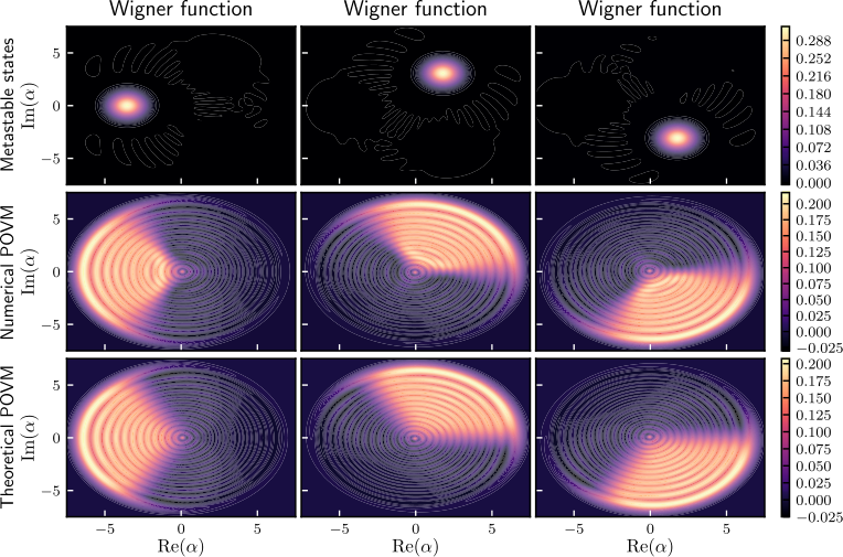
The problem of the previous POVM is the following: our goal is to identify if our system can work as an associative memory, i.e. a state converges to the most similar lobe, but this measure does not permit us to distinguish whether the state is actually over the lobe or in some region nearby.
Therefore, we propose the unambiguous measure which is used for -ary phase-shifted keys Izumi et al. 2012; Becerra et al. 2013. These types of strategies are characterized by the addition of an extra projector that captures all states different from our targets Rudolph et al. 2003, in our case, the lobes. Hence, assuming perfect detector efficiency and no optimization of the displacements, we have and which satisfies (). An example of the Wigner representation for is given in the first row of Fig. S8. In this way, when the -th operator triggers, we are certain that the state was over the -th lobe. In any other situation, the inconclusive operator will be selected.
In both cases, the probability of measuring the correct lobe at a time is where . Here, is the estimation of the most similar lobe at time that is determined using the trace norm, i.e. . Then, we average over random initial coherent states with and phase to avoid biases over particular states. Using this, we obtain the total success probability of identifying the lobe as .
S6 Critical storage capacity
The storage capacity quantifies the density of patterns that can be stored over the size of the system. In the standard HNN, the Hebbian rule is used to encode the patterns in the connections between the spins forming the network. However, it was shown that using this rule only patterns could be stored and retrieved correctly Amit et al. 1985.
In our case, the number of patterns is determined by , the power of the driving, while the size of the system is infinite (). However, only the lowest levels of the Fock space are excited once restricted to the metastable manifold Lörch et al. 2019. Therefore, we can truncate the Hilbert space to a level determining the maximum occupation number that cannot be neglected. Hence, assuming the states in the metastable manifold are coherent and the occupation number follows a Poisson distribution with mean , we have where is an arbitrary numerical accuracy threshold. This leads to the immediate definition of which corresponds to the dashed lines in Fig. 4(b).
This would mean that for small we could have a larger storage capacity compared to the HNN. Of course, this is not realistic as for low (small ) the lobes become indistinguishable, and thus, the success probability becomes . Consequently, we defined a scaled version of that takes into account the separation between lobes, this is
| (S15) |
where is the fidelity between two neighbouring lobes that depends on and . We note that as a consequence of the symmetry, the lobes are identical to each other so the fidelity is equal for all . The final result is that for which correctly describes the impossibility of measuring the lobes independently.
In comparing with the Hebbian capacity we would like to mention two points. First, it is the most well-known and established critical value for associative memories. Second, most practical examples that we encountered in the literature store few amount of patterns, even though the system size is large. For instance, Fuchs and Haken 1988 uses classical neurons to store patterns () and Fiorelli et al. 2020 uses quantum spins to store patterns (). Further, Marsh et al. 2021 found numerically that this limit persists with at least neurons.
We emphasize that in our model, corresponds to the effective dimension of the Hilbert space, which is larger than the number of lobes. To see this comparison more clearly, we show in Fig. 4(c) the minimum size of the system for the required number of patterns. There we can see that for the same amount of patterns, the dimension is smaller in our system than the one required by the Hebbian rule.
In the previous approach, we choose the Fock basis to calculate the effective dimension of the Hilbert space. It is possible to argue that in the metastable transient the states inside the metastable manifold form a displaced Fock basis spanned by the extreme metastable states Azouit et al. 2015; Chamberland et al. 2022. In such a case, the effective dimension of the system is exactly , leading to a storage capacity . Hence, the storage capacity saturates to one for large which is convenient to use as it approaches the ideal limit found by Gardner and Derrida 1988. Despite that, restricting the dynamics to the metastable manifold limits the choice of initial states as the initial dynamics are not correctly described on such a basis. In this sense, the choice of the Fock basis is the most prudent option, as it allows the dynamics of any initial state to be studied, and despite this, it displays an advantage over the storage capacity of classical systems.
S7 Wigner representation
Using the states, we aim to build a HNN Hopfield 1982 with a single quantum system that can distinguish between the solutions. The model is dissimilar once compared to the original HNN consisting of a net of coupled spins. However, there exist generalizations of the associative network for continuous space Wilson and Cowan 1972. In this case, the patterns are excitations of the neuronal field . In our system, we can represent the states using the Wigner quasi-probability distribution Carmichael 1999 that constitutes a 2d-field. Then, the patterns are the Wigner representations of the lobes in Eq. 5, . Hence, the evolution of a state is given by
| (S16) |
where is the sigmoid function and the kernel Meccia and Perazzo 2002.
The time evolution of the Wigner representation , for , is given by
| (S17) |
where has the same definition as in Eq. 4.