A dynamical definition of the sphere of influence of the Earth
Abstract
The concept of sphere of influence of a planet is useful in both the context of impact monitoring of asteroids with the Earth and of the design of interplanetary trajectories for spacecrafts. After reviewing the classical results, we propose a new definition for this sphere that depends on the position and velocity of the small body for given values of the Jacobi constant . Here we compare the orbit of the small body obtained in the framework of the circular restricted three-body problem, with orbits obtained by patching two-body solutions. Our definition is based on an optimisation process, minimizing a suitable target function with respect to the assumed radius of the sphere of influence. For different values of we represent the results in the planar case: we show the values of the selected radius as a function of two angles characterising the orbit. In this case, we also produce a database of radii of the sphere of influence for several initial conditions, allowing an interpolation.
On peut donc, dans le calcul des perturbations d’une comète qui approche très-près d’une planète, supposer à la planète une sphère d’activité dans laquelle le mouvement relatif de la comète n’est soumis qu’à l’attraction de la planète, et au-delà de laquelle le mouvement absolu de la comète autour du soleil n’est soumis qu’à l’action du soleil (P. S. Laplace, Traité de Mécanique Céleste)
1 Introduction
The concept of gravitational sphere of influence of a celestial body was first introduced by Laplace 1805 to investigate close encounters of comets with Jupiter and the Earth. In particular, Laplace applied his theory to the study of Lexell’s comet which, in the second half of the 18-th century, had close encounters with Jupiter and the Earth, producing important changes in its orbital elements. Le Verrier 1844; Le Verrier 1848; Le Verrier 1857 was able to describe the possible changes in the elements (Valsecchi et al. 2003; Valsecchi 2007, see), introducing a first simple version of the Line of Variation (Milani et al. 2005a; Milani et al. 2005b, see).
The gravitational effect of a planet on the motion of a small body was also studied by Tisserand 1889b for the capture of parabolic comets, and by Fermi 1922 in the context of hyperbolic encounters.
Opik 1976 introduced a model of close encounters, allowing to explicitly compute the changes in the orbit of the small body after the encounter. In his model, the encounters are instantaneous, with intersecting orbits. This mechanism was later generalised by Valsecchi et al. 2003 for instantaneous encounters between objects on orbits with non-zero minimum distance.
The patched-conic technique is a further generalisation that allows the encounter to last for a non-zero time interval, see Bate et al. 1971.
Besides the motion of natural bodies, the idea of sphere of influence is also useful in the study of planetary flybys of artificial bodies, like a spacecraft. This was first investigated by Crocco 1956, who studied the possibility of an Earth-Mars-Venus-Earth trajectory using the patched-conic technique.
The definitions of radius of sphere of influence that are commonly used for a planet are the following (see Appendix A):
| (1) | ||||
| (2) |
where is the mass of the Sun, and are respectively the mass and the heliocentric distance of the planet. In the case of the Earth we have
Both definitions (1), (2) give a value of the radius depending only on the mass ratio and on the distance between the planet and the Sun. The same holds true for a less-known definition of sphere of influence given by Chebotarev 1964. However, from more recent studies it results that the classical definitions based on the mass ratio are not always suitable to be employed for the patched-conic technique. Araujo et al. 2008 performed a numerical study showing that the definition of sphere of influence should also depend on the initial relative velocity between the planet and the small body. The authors give an empirical law for the radius of the sphere, but their definition is not applicable to the Earth. Through a numerical study Amato et al. 2017 show that the patched-conic approximation is more accurate by employing a sphere of influence different from classical ones, which however depends on the specific physical problem. In particular, for the Sun-Earth problem they found that the most suitable radius lies between and .
This ambiguity on the definition of the sphere of influence, confirmed by the recent works, is a well-known issue. Laplace himself observed that it is possible to take larger values of the radius of the sphere with respect to the one computed from his formula, and still obtain good results:
On peut même beaucoup augmenter le rayon de cette sphère, sans qu’il en résulte d’erreur sensible. (Laplace 1805, Chap. 2, Book IX)
The purpose of this paper is to unravel the ambiguity and determine the most suitable sphere of influence for the Earth-Sun problem for the patched-conic method, such that the main features of a close encounter and of the post-encounter trajectory are well reproduced. In light of the results cited above, our definition takes into account also the position and velocity of the small body.
The paper is organized as follows. After setting the notation and recalling some basic properties of the restricted three-body problem in Section 2, we describe some features of close encounters in Section 3. We discuss the patched-conic method in Section 4. In Section 5 we introduce the procedure used to define our sphere of influence focusing on the planar case. Some conclusions and a comparison with the classical definitions and are presented in Section 6. Additional material is included in the Appendix, where we also discuss the 3-dimensional case.
2 Dynamical model
For our purpose, we take the dynamical model of the circular restricted three-body problem (CR3BP). We consider a small body, modelled as a massless particle, moving under the gravitational influence of the Sun and the Earth, also called primaries of the problem, see Koon et al. 2011. The primaries are assumed rotating on circular orbits around their common centre of mass.
We make the system non-dimensional. Let and be the masses of the Sun and the Earth. The is chosen as unit of mass. In this way, the non-dimensional masses of the Sun and the Earth are respectively and , where
The distance between the Earth and the Sun is taken as unit of length. Finally, the unit of time is set so that the orbital period of the Earth and the Sun around their centre of mass is equal to . Thus, the universal constant of gravitation becomes equal to .
Let us consider a barycentric synodic reference frame rotating with angular velocity equal to the mean motion of the Earth and the Sun, i.e. equal to . The -plane corresponds to the plane of motion of the primaries. The -axis lies on the line passing through the primaries and it points towards the Earth. The -axis has the direction of the angular momentum of the primaries. In this reference frame the coordinates of the Sun and the Earth are and , respectively.
The Hamiltonian function of the CR3BP is
| (3) |
where
| (4) |
is the distance between the particle and the centre of the Sun, and
| (5) |
is the distance between the particle and the centre of the Earth. In the Hamiltonian function, , , are the momenta conjugated to , , , and fulfil
is an integral of motion. In particular,
| (6) |
is called Jacobi integral. This quantity can be expressed in two alternative forms, employing the heliocentric and geocentric Keplerian osculating elements of the small body:
| (7) |
where are the heliocentric semi-major axis, eccentricity and inclination and is the angle between the small body and the planet seen from the Sun;
| (8) |
where are the geocentric semi-major axis, eccentricity and inclination, and is the angle between the small body and the Sun seen from the planet. In Appendix B we show the computations leading to the three expressions for given in (6), (7) and (8).
3 Close encounters
The orbit of the small body can be approximated as a Keplerian planetocentric hyperbola when it is close to the Earth and it is not captured by the gravitational attraction of the planet. Indeed, in the neighbourhood of the planet, the gravitational influence of the Sun becomes negligible. With this hypothesis, in the following we discuss some general properties of close encounters.
3.1 Types of encounters
We classify close encounters on the basis of two quantities in the framework of the CR3BP:
- 1.
the minimum distance between the planet and the small body;
- 2.
the magnitude of the relative velocity of the small body at the time corresponding to the minimum distance .
In particular, we distinguish between deep and shallow encounters depending on the values of , and between fast and slow encounters depending on the value of .
Let us consider the osculating Keplerian orbit at . The following relations hold between and , where is the magnitude of the asymptotic velocity of the hyperbolic orbit and is its impact parameter (Valsecchi et al. 2003, see):
| (9) |
From relations
we obtain
| (10) |
so that we can write (9) as
| (11) |
Here, , . Relation (10) implies that for a fixed value of , the eccentricity is increasing if is increasing. Let us also remark that from relation , where is the deflection angle (see Fig. 2), we obtain that the greater the eccentricity is, the less the trajectory is curved. As a consequence, for a fixed value of , faster and slower encounters correspond to more straight and more curved hyperbolic trajectories, respectively. In Figure 3 we draw a sketch of the four possible cases for the trajectories. We will see in Section 3.1.1 that, depending on the value of the Jacobi constant , some of these combinations will not be possible.
3.1.1 Estimates for
We derive optimal estimates for the values of the geocentric eccentricity at depending on a chosen value of the Jacobi constant .


Let be the osculating inclination, longitude of the node and argument of perigee at . The distance from the Sun is
with
where is the longitude of the Earth. At the minimum geocentric distance along the 3-body orbit, equation (8) can be written as
with
| (12) |
From (3.1.1) we get that for , given and , the possible values of are simply
Instead, for , we get the possible values of by solving
Then, we have with
| (13) |
These are acceptable, non-spurious solutions if and if
Moreover, since we are looking for hyperbolic orbits, we ask that the condition is also satisfied. The possible values of as a function of the minimum distance are shown in Fig. 4 for . Here, we can see different possibilities depending on . For , is the only acceptable solution for all values of and the minimum and maximum values of increase as increases. For larger values of , the solutions can become acceptable starting from a certain value of . In this way, we can have hyperbolic orbits with small eccentricities for greater than some that depends on . We also note that decreases as increases, so that for values of very close to 3 there are orbits with small geocentric eccentricities for all values of the perigee distance .
3.2 The Tisserand parameter
It is well known that there exists a quantity, called Tisserand parameter, which takes almost the same value before and after a close encounter with a planet (Tisserand 1889a). Indeed, it remains almost constant when the small body is far from the planet, it decreases as the small body approaches the planet and then stabilises on a value that is very close to the pre-encounter one. The typical behaviour of the Tisserand parameter during a close encounter is shown in Fig. 5.
In terms of the orbital elements, the Tisserand parameter, denoted by , is written as
| (14) |
In this section we derive an upper bound for the time-derivative of . Our aim is to find a distance from the Earth, depending on the Jacobi constant, where the effect of the planetary gravitational attraction is negligible. For the optimisation process described in Section 5 we will consider initial conditions that depend on . From (7) and (14) we get
In the synodic barycentric reference frame, the position of the small body can be written in terms of the spherical angles and as
where is the geocentric distance. From (6) we see that the norm of the velocity is given once the value of the Jacobi integral and the position of the small body are fixed.
Then, the velocity vector of the small body can also be described by two angles , so that
The time derivative of is
Since , we have
Thus,
Let us call the constant value assumed by the Jacobi integral . Knowing that
| (15) | |||
| (16) |
from (6) we obtain
with
It holds , where
We have for every value of , considering that , with the Earth radius.
We can now look for values of the geocentric distance at which the Tisserand parameter remains approximately constant, by solving
| (17) |
with some small quantity. This bounding condition corresponds to the inequality
| (18) |
where
| (19) | ||||
with . Let us consider and set . From (19) we have
therefore for any value of there exists at least one positive solution of . Let be the positive solutions of and . From the implicit function theorem we know that
We have
which is negative for . Moreover,
From a numerical evaluation we get , therefore it must be . We then have . Furthermore, , so that for all . Since , we get that there exists for all . We then also have . Therefore, we conclude that and for every . We take as the smallest positive value of that satisfies inequality (18), i.e. . In Fig. 6 we show the evolution of as varies in the interval .
4 Patched-conic Method
Planetary close encounters can be studied by means of the patched-conic approximation. The small body is modelled as a massless particle, travelling along a heliocentric Keplerian elliptic orbit before and after the encounter. The encounter occurs inside the sphere of influence of the Earth, where the orbit of the small body is a geocentric Keplerian hyperbolic orbit.
By adopting the synodic barycentric reference frame introduced in Section 2, the Hamiltonian function of the heliocentric Kepler problem is
| (20) |
with defined in (4). Similarly, the Hamiltonian function of the geocentric Kepler problem is
| (21) |
with defined in (5). In the patched-conic method, when the small body is far from the planet we only consider the gravitational influence of the Sun, so that the trajectory of the small body is simply described by a Keplerian elliptic orbit resulting from the dynamics associated to the Hamiltonian (20). In case of close encounters with the Earth, if the geocentric distance of the small body is small enough, the gravitational attraction of the planet becomes dominant. When this happens, we instantaneously change the centre of gravity: the small body is now only affected by the influence of the Earth and its trajectory is simply given by a Keplerian hyperbolic orbit resulting from the Hamiltonian dynamics associated to (21). Then, once the small body gets far enough from the planet, we switch back again to the pure Sun-particle two-body problem.
4.1 Effective deflection
Let be the geocentric hyperbolic orbit inside the sphere of influence. will depend on the chosen radius of the sphere of influence. Let us denote by the unit vector of the geocentric velocity at the exit point from the sphere of influence, by the unit vector of the hyperbolic asymptotic velocity, and by the angle between and .
Here, we derive the relation between , where and are the pericentre distance and the eccentricity of .
The position and velocity along are given by
with the true anomaly, the geocentric distance and its derivative with respect to . In particular,
The squared magnitude of the velocity along the hyperbolic orbit is
The asymptotic value of the true anomaly is determined by
so that
Instead, the value of the true anomaly at the exit of the sphere of influence is determined by
Therefore, the normalised velocity can be written as
We note that , where is the deflection angle introduced in Section 3.1. The angle between , corresponds to half the angle of missed deflection, that we denote by , so that
5 A new definition of sphere of influence
In this section we describe the numerical method used to define a suitable radius of the sphere of influence, depending on the state variables of the small body. From now on we restrict our analysis to the planar problem.
5.1 Initial Conditions
Let us fix the value of the Jacobi integral and the initial distance between the particle and the Earth. We select such that the variation of the Tisserand parameter is small. In this way, at the initial time , the motion of the particle can be approximated by a Keplerian orbit around the Sun. We choose
| (22) |
with defined in Section 3.2 and ; is set in order to have for all (see relation 17). The initial positions of the particle are selected on the circle
| (23) |
Given an initial position , the norm of the velocity is completely determined by the value of the Jacobi integral . Indeed, from equation (6), we have
| (24) |
where , see (4). We can prove that for and for every relation (24) gives . Let us set . We have
where
The function attains its minimum at . Indeed,
and
Thus, we get
With the assumptions made in Section 3.2 (see Fig. 6) and from (22), we have , so that
We can parametrize the initial conditions with two angular coordinates and . Let us consider a geocentric synodic reference frame with the same orientation of : is the angle between the -axis and the initial position of the particle, is the angle between the initial position of the particle and its velocity, see Fig. 7. The initial conditions in barycentric synodic coordinates are given by
Since we are interested in close encounters, the initial velocities are selected in order to obtain trajectories entering the circle . This means taking . The set of initial conditions is determined by considering a regularly-spaced grid on the -plane.
5.2 Computation of the 3-body orbit
For each initial condition, we propagate the orbit in the CR3BP. The propagation is interrupted either when the particle reaches again the initial distance from the planet or when a maximum propagation time is reached. In the following, we denote by the orbit computed for each initial condition, where and is the time at which the propagation is stopped.
Since the particle can get very close to the Earth, the propagation is performed using the Levi-Civita regularization (Stiefel and Scheifele 1971). We introduce the variables through the canonical transformation
| (25) | ||||
| (26) | ||||
| (27) | ||||
| (28) |
and a fictitious time through relation
The regularized Hamiltonian is
| (29) |
where is the constant value of the Hamiltonian function in (3) evaluated at the initial conditions .
The equations of motion are then
with the primed quantities corresponding to the derivatives with respect to the fictitious time .
5.3 Optimisation process
For each initial condition and given the associated 3-body orbit , we search for minimizing the target function defined as
| (30) |
where is the orbit obtained by applying the patched-conic method with a sphere of influence of radius and and are respectively the times of minimum geocentric distance of the 3-body orbit and of the patched-conic orbit. Let us remark that and are generally different. Because of the three different terms of , the optimisation procedure allows us to determine a patched-conic orbit with the following features: it is close to the 3-body orbit in the phase space over the whole time interval ; its final state is similar to the final state of the 3-body orbit; its state at the perigee is similar to the state of the 3-body orbit at . The domain of is defined as
We remind that is the minimum geocentric distance reached by the particle along the 3-body trajectory. The upper bound is chosen as a distance from the Earth where the gravitational influence of the planet is negligible with respect to that of the Sun. In our computation, we set so that the ratio between the magnitudes of the gravitational attraction of the Earth and the Sun is
If , we assume that there is no close encounter, thus can be entirely approximated by a Keplerian heliocentric orbit. We summarise the steps performed to determine :
- 1.
sample the domain with equi-spaced points , for ;
- 2.
compute for each .
- 3.
evaluate and identify the subset of containing the minimum point of ;
- 4.
re-sample the interval with points for ;
- 5.
compute , and evaluate for all . Comparing the results, choose such that
(31)
It is important to remark that, for some in step (i) above, we could obtain a trajectory which does not enter the sphere of influence: in that case, corresponds to a Keplerian heliocentric orbit. The same can occur for some in step (v). Moreover, we are not interested in encounters that last a very short time: in these cases, the patched-conic method would give small corrections which can be neglected. Thus, we avoid the orbit patching and use a purely heliocentric orbit if
| (32) |
at the entrance of the sphere of influence. We use : this choice will be discussed in Section 6.
During the procedure, if we identify different local minimum points of with the same minimum value, we select the smallest one. Furthermore, to reduce the computational cost, if for some the value of the target function becomes larger than a certain threshold, we avoid the computation of the values of , for . In our computation we use the threshold
Finally, we check whether the selected is such that is a purely Keplerian heliocentric orbit. In that case, we set . Let us remark that the method can not be applied if the trajectory of the particle is such that the geocentric distance has multiple local minima lower than . This phenomenon typically occurs for high values of the Jacobi constant when the initial osculating semi-major axis and eccentricity are approximately close to 1 and 0, respectively, i.e. when the 3-body orbit is close to the orbit of the Earth. Sometimes, the same phenomenon is instead related to a gravitational capture by the Earth. In all these cases, we discard the initial conditions, as it is not possible to apply our procedure to compute a sphere of influence.
5.4 Selection of the radius
For all initial conditions such that , the radius of the sphere of influence is set equal to zero. Otherwise, we compute the Keplerian heliocentric orbit with and evaluate the quantity
| (33) |
where is the time of minimum distance of the small body from the planet along the heliocentric orbit. Then we compare the value of with . If we set , meaning that the best approximation is given by the heliocentric orbit. Otherwise we select .
5.5 Interpolation
With the method described in Section 5 we computed a database of values of for each point of a grid in the plane and for different values of the Jacobi constant , with . To obtain a value of for each possible data in the domain
we apply the trilinear interpolation method described below.
Let be the values of for which we apply the optimisation method described above and let be the initial conditions we have considered. Any point with
is inside the rectangular prism
This method computes by weighing the known values of at the vertices of the prism . The planes passing through and parallel to the faces of , divide this prism into eight smaller ones. The value at each of the eight nodes is weighted by the volume of the smaller prism diagonally opposite to the node, that is
where is the volume of .
The process is reduced to a simple bilinear or linear interpolation in case one or two of the values coincide exactly with the values used to generate our database.


6 Results and discussion
For fixed values of the Jacobi constant, following the procedure of the previous section, we compute for each point of a grid in the plane. In Fig. 8 left, we show our results for some values of , chosen in the most significant range for near-Earth asteroids11 1 we used the NEODyS database https://newton.spacedys.com/neodys, i.e. . Warmer colours correspond to larger values of . The dark-blue region corresponds to , i.e. where a heliocentric Keplerian orbit is chosen. In Fig. 8 right, we plot the values of the minimum geocentric distance reached along the 3-body propagation. Warmer colours correspond to larger values of . The thin, dark-blue wave represents the set of initial conditions leading to very close encounters or collisions. The dashed white line corresponds to the collision curve, i.e. the set of points for which the 3-body trajectory passes through the centre of the Earth (in Appendix C we explain the procedure to compute it). In the bottom images of Fig. 8, the white region corresponds to points where our method cannot be applied.
Comparing the images on the right with those on the left we notice that our method gives in the region surrounding the collision curve. This result was expected, since this is precisely the region where the small body gets closest to the Earth. In Fig. 9 we show the values of , defined in (30), replaced by (see 33) if . Warmer colours represent higher values of . For the considered values of , in the neighbourhood of the collision curve, achieves the highest values.


In general, the method provides a patched-conic orbit that allows us to reproduce some significant features of the 3-body orbit with a reasonable error, such as the post-encounter osculating semi-major axis and eccentricity at . To give an example, in Fig. 10 we show the relative error of these quantities for . Note that the maximum value of the relative error is less than for the semi-major axis and less than for the eccentricity. Through our method it is usually also possible to reproduce with sufficient accuracy the minimum geocentric distance and the osculating geocentric eccentricity at . An example can be seen in Fig. 11 where we show the relative errors and for . For of points we have and for .

In Fig. 12 we plot, in the plane, the percentage of achieved deflection computed by considering , where is the missed deflection, see Section 4.1. The minimum percentage obtained in the case considered in Fig. 12 is . Although this is very low, the percentage of achieved deflection gets higher as decreases. There is a region around the collision curve where the achieved deflection is very close to the maximum possible one. We argue that this is where it is important to have a high deflection percentage. Indeed, here the planetocentric eccentricity is lower and therefore the trajectory of the small body is significantly deflected by the Earth. With our method we are then able to reproduce this effect.

In Fig. 13 left we show the time spent inside the sphere of influence. Here, we selected , but the behaviour is similar for the other values of the Jacobi constant. Warmer colours denote longer encounter times, and the dark-blue region corresponds to . We can clearly distinguish the bright-yellow region, corresponding to encounters that last more than 100 hours. Outside this region the duration of the encounter is considerably smaller. By comparison with Fig. 13 right, we can notice that the time spent inside the sphere of influence is very short when the ratio is close to . If we imposed a smaller value of in (32), the region in which would be larger, replacing part of the dark-blue region. In these cases, the patched-conic method gives only a slight improvement with respect to a simple heliocentric Keplerian propagation. This can be inferred from the example in Fig. 14. On the left, we show the graph of in the neighbourhood of its minimum value for a point such that . Note that the minimum is very close to and it belongs to a very small interval of values of where is not smooth. On the contrary, the difference between the minumum of and is significant for points in the region near the collision curve, as shown in Fig. 14 right. After performing some tests, we chose , but higher values seem suitable too.
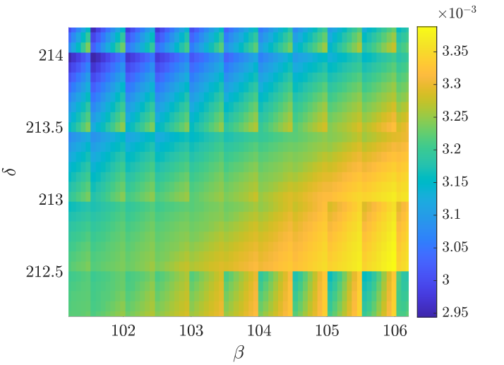
Using the interpolation technique explained in Section 5.5 we can compute for values of different from the nodes of our database. In Fig. 15 we display the target function (30) computed with interpolated values of . In this example, we consider a region close to the collision curve. Note that remains confined to small values. In Fig. 16 we compare the radius obtained by interpolation with Hill’s and Laplace’s radii (, ) by plotting the differences
In this example we can see that both quantities above are always negative. This means that, according to our selected norm, the interpolated gives a better approximation than both Hill’s and Laplace’s radii. In Fig. 17, we repeat the same experiment for points selected in a region farther from the collision curve, where . The results obtained are not as good as in the previous case. This is a consequence of the features of : as already shown, the minimum of typically belongs to a very small neighbourhood of values of where the function is not smooth. Thus, computing through an interpolation process can produce a significant error. We could reduce the error by increasing the density of the points in the database. However, this would also imply increasing significantly the computational cost required for the generation of the grid, which is not worthwhile since the minimum of is slightly smaller than . This difficulty related to the application of the interpolation process is an additional reason for increasing the value of .
Our database is available at the webpage http://adams.dm.unipi.it/cmg/rsoi/rsoi.html.


7 Conclusions
In this work we searched for an appropriate choice of the radius of the sphere of influence of the Earth within a planar patched-conic model. We developed an optimisation method, minimizing a target function that depends on the possible radius of the sphere of influence. This target function is made up of three components: 1) the sup-norm of the difference between the 3-body and the patched-conic orbits computed over a time interval including the encounter; 2) the distance between the final states of the two orbits; 3) the norm of the difference between the states at the minimum geocentric distance. This procedure was repeated for a grid of different initial conditions, defined by the Jacobi constant and by two angles, and allowed us to construct a database of values of . The resulting data can be used to define a sphere of influence for generic initial conditions, by interpolation. We found that the best choice of is typically close to Hill’s radius , or larger. This is consistent with the outcomes of Amato et al. 2017. Some exceptions can be found for initial conditions leading to a very deep close encounter, or a collision. Our procedure can be applied to the 3-dimensional case, as described in Appendix D. However, the higher number of initial conditions that we should consider in this case requires some care, both in the implementation and in the data management. In future, it would also be interesting to investigate the cases to which our method cannot be applied to more deeply understand the phenomena causing the failure.
Acknowledgments
This work was partially supported through the H2020 MSCA ETN Stardust-Reloaded, Grant Agreement Number 813644. CG, GFG and GB also acknowledge the project MIUR-PRIN 20178CJA2B “New frontiers of Celestial Mechanics: theory and applications". The authors also acknowledge the GNFM-INdAM (Gruppo Nazionale per la Fisica Matematica).
Appendix A Classical definitions of the sphere of influence
The classical definitions of the sphere of influence are
- 1.
- 2.
Hill’s sphere, defined in equation (2), approximating the distance from the planet to the Lagrangian point (Chebotarev 1964).
In Chebotarev 1964, the author introduced a further definition of sphere of influence, corresponding to "the region of space within which the attraction of the planet is greater than solar attraction", see also Souami et al. 2020. The radius of Chebotarev’s sphere is
As shown in Souami et al. 2020, relation
| (34) |
holds when . In particular, if and if . Since the ratio between the mass of Jupiter and that of the Sun is about 0.001, (34) is true for all solar system planets.
A.1 Laplace’s sphere
We derive the radius of Laplace’s sphere of action following H. 1999. We consider the Sun-Earth problem, but what follows is valid for any planet. We adopt the same non-dimensional system described in Section 2, and we denote by the heliocentric position vector of the Earth and by and the position of the small body with respect to the Sun and the Earth, respectively. Let
The small body is approximated as a massless particle. We can consider two perturbed two-body problems: the Sun-particle problem perturbed by the Earth and the Earth-particle problem perturbed by the Sun. These are described by
| (35) | ||||
| (36) |
where , are the two-body accelerations and , are the perturbing accelerations.
Laplace’s sphere of influence is obtained by finding the geocentric distance where the ratios between two-body and perturbing accelerations in (35) and (36) are the same, that is
This condition becomes
Noting that
we can write
so that
Since , the sphere of influence will be much closer to the Earth than to the Sun, so that we can assume and therefore expand in power series of . Noting also that
| (37) |
we have
and
Then, we can write
and
Considering that , we simply approximate it with and finally get the value of the radius of Laplace’s sphere of influence
The approximation performed is typical in modern works, see for example H. 1999; on the contrary, Laplace 1805 chose the alternative , leading to
A.2 Hill’s sphere
In the planar CR3BP, the region of allowed motion is given by the Hill region. Depending on its energy, the small body can be free to move everywhere, or be confined to smaller regions. In particular, if its energy is lower than the energy associated to the Lagrangian point , then the region of possible motion is closed and a small body in the vicinity of the planet is bound to stay close to the planet.
The definition of the radius of the Hill sphere of influence comes from an approximation of the distance of the Lagrangian point from the planet.
Equilibrium points are found by solving the system
From the first two equations we get . Setting to search for collinear Lagrangian points, from the third equation we get
Let . We notice that for the Lagrangian point located between the primary and the secondary body. The equation above yields an explicit expression for . For this is
which, after expanding around , becomes
The distance of the point from the planet is obtained by solving the equation above in power series of
see (Szebehely 1967). The radius of Hill’s sphere corresponds to the first term of this expansion.
A.3 Chebotarev’s sphere
Appendix B Jacobi integral
B.1 Barycentric inertial coordinates
As a first step, it is convenient to consider the coordinate change defined by
| (39) |
where is the longitude of the Earth, given by
with the non-dimensional time, its initial value and the value of at . Note that if and the value of the longitude corresponds to the value of the non-dimensional time. The coordinates are barycentric inertial coordinates. Differentiating (39) with respect to gives the transformation of the velocity components:
| (40) |
From (6), applying the transformations (39) and (40), we obtain the Jacobi integral as a function of the barycentric inertial variables:
with
It is straightforward in the new variables to express the heliocentric position and velocity vectors and of the small body, as well as the planetocentric ones, and . It holds
| (41) | ||||
| (42) | ||||
| (43) | ||||
| (44) |
B.2 Heliocentric elements
B.3 Planetocentric elements
Let us assume that the osculating planetocentric elements correspond to the orbital elements of hyperbolic trajectories, i.e. they are such that . Then, we have
and
and
we obtain
| (47) |
and
| (48) |
Substituting (47) and (48) in (B.1) and simplifying, we find
| (49) |
Equation (8) is obtained using and
in (49), with the angle between the small body and the Sun seen from the Earth.
Appendix C Collisions
Let us fix a value of the Jacobi integral and an initial distance from the Earth, as in Section 5.1. We describe the procedure applied to compute the collision curve displayed in Fig. 8, defined by the values of the angles such that the corresponding 3-body trajectory passes through the centre of the Earth. In the regularised variables, this condition corresponds to
for some value of the fictitious time. Let
and assume that is a collision condition, i.e. . From the implicit function theorem, if the Jacobian matrix
| (50) |
is non-singular in , then there exists a local parametrization
of the collision curve defined in a neighbourhood of , such that
Moreover, the tangent vectors to the collision curve can be written as
In our case the Jacobian matrix (50) can be computed as
where
is the state transition matrix of the system with Hamiltonian (see 29), and stands for vector transposition. Moreover,
To compute the collision curve, we perform the following steps: (i) we select a starting point that leads to a collision at time ; (ii) we move slightly away from along the direction of the tangent vector and look for a new collision point in the direction orthogonal to ; (iii) we iterate the process once the new collision point has been found.
Appendix D 3-dimensional case
To apply the method described in Section 5 to the 3-dimensional problem, a few changes are required. In particular, it is necessary to extend the set of initial conditions and use the KS regularisation for the 3-body propagation. Moreover, since the initial conditions will be described by more than three variables, a multi-variate interpolation method is necessary. More details on the selection of the initial conditions and a brief summary of the KS regularisation are reported below.
D.1 Initial Conditions
In the 3-dimensional configuration space, the initial position of the particle must be selected on the sphere defined as
As in the planar case, for any initial position the norm of all possible velocities is completely determined once the Jacobi constant has been fixed:
| (51) |
where (see 4). In the 3-dimensional case, especially for higher values of , we may have points for which relation (51) gives : these points must be excluded from the domain.
Four angular coordinates , , and are required to parametrize the initial conditions. The angles and are the spherical coordinates with respect to the geocentric synodic reference frame and are used to define the position vector. Consider now a reference frame centred at the position of the small body , obtained through the transformation
The angles and are spherical coordinates with respect to the reference frame and are used to define the velocity vector. Thus, the initial conditions in the barycentric synodic variables are given by
Note that if and , we obtain the initial conditions of the planar problem. Also for the 3-dimensional problem, we need to consider to obtain trajectories entering the sphere . The set of initial conditions is determined constructing a regularly-spaced grid in the 4-dimensional space .
D.2 Propagation with KS variables
For the 3-dimensional problem, we need to perform the propagation using the variables of the Kustaanheimo-Stiefel regularisation (Stiefel and Scheifele 1971). We introduce these variables through the transformation
where , and
We also introduce the fictitious time through the differential relation
Let us denote with a prime the derivative with respect to . For the fixed value of the Jacobi integral , the equations of motion are
where
As for the planar problem, after the propagation we transform the orbit back to barycentric synodic coordinates.
References
- Amato et al. [2017] D. Amato, G. Baù, and C. Bombardelli. Accurate orbit propagation in the presence of planetary close encounters. Monthly Notices of the Royal Astronomical Society, 470(2):2079–2099, Sept. 2017. doi: 10.1093/mnras/stx1254.
- Araujo et al. [2008] R. A. N. Araujo, O. C. Winter, A. F. B. A. Prado, and R. Vieira Martins. Sphere of influence and gravitational capture radius: a dynamical approach. Monthly Notices of the Royal Astronomical Society, 391(2):675–684, Dec. 2008. doi: 10.1111/j.1365-2966.2008.13833.x.
- Bate et al. [1971] R. R. Bate, D. D. Mueller, and J. E. White. Fundamentals of Astrodynamics. Dover publications, 1971.
- Chebotarev [1964] G. A. Chebotarev. Gravitational Spheres of the Major Planets, Moon and Sun. Soviet Astronomy, 7:618, Apr. 1964.
- Crocco [1956] G. A. Crocco. One year exploration trip earth-mars-venus-earth. Proc. VII International Astronautical Congress, page 227, 1956.
- Fermi [1922] E. Fermi. Collected papers. 1922.
- H. [1999] B. R. H. An introduction to the Mathematics and Methods of Astrodynamics. AIAA Education Series, New York, 1999.
- Koon et al. [2011] W. S. Koon, M. W. Lo, J. E. Marsden, and S. D. Ross. Dynamical Systems, the Three-Body Problem, and Space Mission Design. 2011.
- Laplace [1805] P. S. Laplace. Traité de Mécanique Céleste, volume IV. Courcier, 1805.
- Le Verrier [1844] U.-J. Le Verrier. Sur la comète de m. faye ; Lettre de M. Le Verrier à M. Cauchy. Comptes Rendus de l’Académie des Sciences, 19:982, 1844.
- Le Verrier [1848] U.-J. Le Verrier. Mémorie sur de la comète périodique de 1770. Comptes Rendus de l’Académie des Sciences, 26:465, 1848.
- Le Verrier [1857] U. J. Le Verrier. Thórie de la comete periodique de 1770. Annales de l’Observatoire de Paris, 3:203–270, Jan. 1857.
- Milani et al. [2005a] A. Milani, S. R. Chesley, M. E. Sansaturio, G. Tommei, and G. B. Valsecchi. Nonlinear impact monitoring: line of variation searches for impactors. Icarus, 173(2):362–384, Feb. 2005a. doi: 10.1016/j.icarus.2004.09.002.
- Milani et al. [2005b] A. Milani, M. E. Sansaturio, G. Tommei, O. Arratia, and S. R. Chesley. Multiple solutions for asteroid orbits: Computational procedure and applications. Astronomy & Astrophysics, 431:729–746, Feb. 2005b. doi: 10.1051/0004-6361:20041737.
- Opik [1976] E. J. Opik. Interplanetary encounters : close-range gravitational interactions. Elsevier, Amsterdam, 1976.
- Souami et al. [2020] D. Souami, J. Cresson, C. Biernacki, and F. Pierret. On the local and global properties of gravitational spheres of influence. Monthly Notices of the Royal Astronomical Society, 496(4):4287–4297, Aug. 2020. doi: 10.1093/mnras/staa1520.
- Stiefel and Scheifele [1971] E. Stiefel and G. Scheifele. Linear and Regular Celestial Mechanics. Springer–Verlag, 1971.
- Szebehely [1967] V. Szebehely. Theory of orbits. The restricted problem of three bodies. Academic Press, 1967.
- Tisserand [1889a] F. Tisserand. Mémoires et observations. Sur la théorie de la capture des comètes périodiques. Bull. Astron., Sér. I 6:289–292, 1889a.
- Tisserand [1889b] F. Tisserand. Traité de Mécanique Céleste, volume IV. 1889b.
- Valsecchi [2007] G. B. Valsecchi. 236 years ago… Proc. IAU Symposium 236, pages xvii–xx, 2007.
- Valsecchi et al. [2003] G. B. Valsecchi, A. Milani, G. F. Gronchi, and S. R. Chesley. Resonant returns to close approaches: Analytical theory. Astronomy & Astrophysics, 408:1179–1196, Sept. 2003. doi: 10.1051/0004-6361:20031039.