3D Single Source Localization Based on Euclidean Distance Matrices

We define the $3\times(M+1)$-dimensional positions matrix as $\mathbf{P}=[\mathbf{M}|\,\mathbf{s}]$. The corresponding $(M+1)\times(M+1)$-dimensional EDM $\overline{\mathbf{D}}$ is defined as

This matrix contains the inter-microphone EDM $\mathbf{D}=\left[D^{2}_{i,j}\right]$, with $D_{i,j}=||\mathbf{m}_{i}-\mathbf{m}_{j}||$ the distances between the $i$-th and $j$-th microphones, and the Euclidean distance vector $\mathbf{d}=\left[d^{2}_{1},\dots,d^{2}_{M}\right]^{\textrm{T}}$, with $d_{m}=||\mathbf{m}_{m}-\mathbf{s}||$ the distance between the source and the $m$-th microphone.

In [17, 12], it was shown that an EDM corresponding to a 3D geometry can be transformed to a Gram matrix, whose rank is at most 3, as

where $\mathbf{I}$ denotes the identity matrix, $\mathbf{1}$ denotes a vector with ones, and $\mathbf{e}$ denotes a vector with zeros except for the element corresponding to the reference microphone (chosen as the first microphone without loss of generality), equal to one. The Gram matrix can be written using the relative microphone and source positions $\mathbf{P}_{\textrm{rel}}$ as $\mathbf{G}=\mathbf{P}_{\textrm{rel}}^{\textrm{T}}\mathbf{P}_{\textrm{rel}}$, where the absolute positions $\mathbf{P}$ are related to the relative positions $\mathbf{P}_{\textrm{rel}}$ via a translation which places the reference microphone at the origin, and the remaining array is arbitrarily rotated and/or reflected (preserving the inter-microphone distances). Realizing that the positive semi-definite Gram matrix has at most 3 positive eigenvalues which are not equal to zero, i.e., $\lambda_{1}\geq\dotsc\geq\lambda_{3}\geq 0$ and $\lambda_{4}=\dots=\lambda_{M+1}=0$, the relative positions $\mathbf{P}_{\textrm{rel}}$ can be written using the eigenvalue decomposition of $\mathbf{G}$ as

where $\mathbf{0}_{{3}\times((M+1)-3)}$ is a $3\times((M+1)-3)$ dimensional matrix of zeros and $\mathbf{U}$ denotes the matrix containing the eigenvectors of $\mathbf{G}$. The relative positions $\mathbf{P}_{\textrm{rel}}$ can be aligned with the absolute positions $\mathbf{P}$ using orthogonal Procrustes analysis [13, 12] by aligning the relative microphone positions $\mathbf{M}_{\textrm{rel}}$ with the known microphone positions $\mathbf{M}$. This simultaneously aligns the relative source position $\mathbf{s}_{\textrm{rel}}$ with the absolute source position $\mathbf{s}$.

Defining $\alpha_{s}$ as the distance between the source and the reference microphone (i.e., $\alpha_{s}=d_{1}$), the distance between the source and the $m$-th microphone can be written as

where $\tau_{m,1}(\mathbf{s})$ denotes the TDOA between the $m$-th microphone and the reference microphone. Assuming for now that the TDOAs are known and considering the distance variable $\alpha$, we can define $d_{m}(\alpha)$ similarly to (9), i.e.,

Using $d_{m}(\alpha)$, we can construct the Euclidean distance vector $\mathbf{d}(\alpha)=\left[d^{2}_{1}(\alpha),\dots,d^{2}_{M}(\alpha)\right]^{\textrm{T}}$, the EDM $\overline{\mathbf{D}}(\alpha)$ and its Gram matrix $\mathbf{G}(\alpha)$. As mentioned in Section 3.1, the rank of $\mathbf{G}(\alpha)$ is equal to 3 if $\alpha=\alpha_{s}$. Motivated by the idea of minimizing the rank of a matrix as in [18], we now define the cost function

which considers all but the three largest eigenvalues $\lambda_{i}(\alpha)$ of $\mathbf{G}(\alpha)$. The absolute values of the eigenvalues are used, since it can not be guaranteed that the eigenvalues of $\mathbf{G}(\alpha)$ are positive for all values of $\alpha$ (e.g., in case of a mismatch with the TDOAs). If $\alpha=\alpha_{s}$, then all but the three largest eigenvalues of $\mathbf{G}(\alpha_{s})$ are equal to zero, such that $J\left(\alpha_{s}\right)=0$. The optimal value $\alpha_{s}$ can hence be found as

In practice, the TDOAs, of course, aren’t available, so we now rewrite (10) to take into account the estimated TDOAs. If the source or a microphone is close to a wall or the corner of a room, super-positions of acoustic reflections may lead to peaks in the time-domain GCC-PHAT function (1), which are higher than the peak corresponding to the direct path. Basing the TDOA estimate on these erroneous peaks can result in large errors in the source localization. We propose to consider $C$ candidate TDOA estimates per microphone pair, corresponding to the $C$ highest local peaks in the time-domain GCC-PHAT function. The index $c_{m}\in\{1,\dots,C\}$ denotes the candidate TDOA estimate $\hat{\tau}_{m,1}^{c_{m}}$ between the $m$-th microphone and the reference microphone. This means that the distance variable $d_{m}(\alpha,\hat{\tau}_{m,1}^{c_{m}})$ now becomes a function of the distance variable $\alpha$ as well as the estimated candidate TDOA estimates, i.e.,

Similarly to Section 3.2, we now construct the Euclidean distance vector $\mathbf{d}(\alpha,\hat{\tau}_{2,1}^{c_{2}},\dots,\hat{\tau}_{M,1}^{c_{M}})$, the EDM $\overline{\mathbf{D}}(\alpha,\hat{\tau}_{2,1}^{c_{2}},\dots,\hat{\tau}_{M,1}^{c_{M}})$ and its Gram matrix $\mathbf{G}(\alpha,\hat{\tau}_{2,1}^{c_{2}},\dots,\hat{\tau}_{M,1}^{c_{M}})$, and determine the optimal distance variable $\hat{\alpha}_{s}$ with (11) for all $C^{M-1}$ possible combinations of candidate TDOA estimates, taking the value with the minimal cost, i.e.,

This corresponds to the distance between the source and the reference microphone $\alpha$ and the combination of candidate TDOA estimates which best match with each-other in terms of constructing a 3D geometry. It should be noted that the minimum of (14) is not guaranteed to be 0 like in (11), due to possible estimation errors in the TDOAs. For an exemplary 3D source and microphone constellation with $\alpha_{s}=d_{1}=2.28$ m, Fig. 1 depicts the dependence of the cost function $J(\alpha,\hat{\tau}_{2,1}^{c_{2}},\dots,\hat{\tau}_{M,1}^{c_{M}})$ on the distance variable $\alpha$.

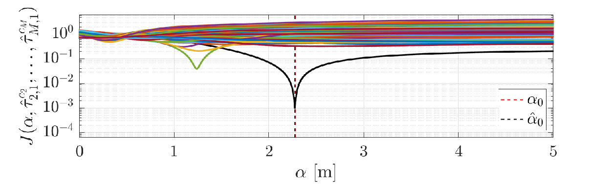
To reconstruct the estimated relative positions $\hat{\mathbf{P}}_{\textrm{rel}}$, only the three largest positive eigenvalues (for which the cost function (14) is minimized) and the corresponding eigenvectors are used in (8). The same alignment procedure is applied as described in Section 3 to map the estimated relative microphone position $\hat{\mathbf{s}}_{\textrm{rel}}$ to the estimated microphone position $\hat{\mathbf{s}}$. An overview of the EDM-based source localization is depicted in Fig. 2.

In practice, the maximization of the SRP functional $\Psi(\mathbf{p})$ in (5), which depends on 3 continuous variables, is approximated through an exhaustive search on a discrete grid $\mathbf{p}^{\prime}$. First, the integral in (4) is approximated by a sum over STFT frequency bins, i.e., i.e.,

with frequency bin index $k\in\{0,\dots,K-1\}$, with $K$ the Fourier transform length, and frame index $l\in\{1,\dots,L\}$. Assuming a static source, the source position is then estimated by maximizing the sum of the SRP-PHAT functionals over $L$ frames, i.e.,

Since we perform a summation over frames in (16), we use instantaneous estimates of $\psi_{i,j}[k,l]$ in (15) (i.e, the expectation operation in (2) constitutes an average over a single frame) in order to not perform two temporal averaging operations.

Exhaustively searching for the 3D source position estimate at a high grid resolution can be computationally demanding. Loosely based on coarse-to-fine region contraction in [6], we first evaluate (16) on a coarse 3D grid and then in the vicinity of a few points where SRP-PHAT yields the highest values, we evaluate the SRP-PHAT functional on a fine grid in those regions.

In the STFT-domain, GCC-PHAT $\psi_{i,j}[k,l]$ is estimated in each frequency bin $k$ and time frame $l$, and the the continuous Fourier transform in time-domain GCC-PHAT is approximated with an inverse discrete Fourier transform for discrete time-lags $n$, i.e.,

To achieve a more precise TDOA estimate, the time-domain GCC-PHAT function $\xi_{m,1}[n,l]$ can be interpolated between the discrete time-lags $n$ with a factor $R\geq 1$. The lower and upper limits of the possible time-lags are dependent on the distances between the microphone pair, i.e., $|n_{m}|<D_{m,1}f_{s}R/c$. Using the interpolated time-domain GCC-PHAT, the sample-delay between the $m$-th and the reference microphone is estimated as

corresponding to the estimated TDOA $\hat{\tau}_{m,1}=\hat{n}_{m}/(f_{s}R)$. Similarly to the previous section, since we perform a summation over frames in (18), we use instantaneous estimates of $\psi_{i,j}[k,l]$ in (17).

For the simulations, we considered a rectangular room with dimensions $6\times{}6\times{}2.4$ m and simulated room impulse responses using the image method [19, 20], assuming equal reflection coefficients for all walls. The $M=6$ spatially distributed microphones were randomly positioned within a cube with cube length 2 m (with a minimum distance of 2 cm between the microphones) and the source was located at one of four fixed distances $\alpha_{c}\in\{0.5,1,2,3\}$ m from the centroid of the microphone positions (in a random direction). For each source distance $\alpha_{c}$, we considered 100 acoustic scenarios, using a 5 s speech signal randomly selected from [21] (with equal probability for a male or female speaker) as the source signal. The reflection coefficients were set for each scenario such that the room impulse responses had an average direct-to-reverberant ratio of approximately $0$ dB over the microphones. This was achieved by setting $T_{60}=0.60\pm 0.14$ s for $\alpha_{c}=0.5$ m, $T_{60}=0.47\pm 0.10$ s for $\alpha_{c}=1$ m, $T_{60}=0.29\pm 0.04$ s for $\alpha_{c}=2$ m and $T_{60}=0.25\pm 0.03$ s for $\alpha_{c}=3$ m. Spherically isotropic multi-talker babble noise was generated using [22] and added to the reverberant speech component in the microphones at 5 dB signal-to-noise ratio. The sampling frequency was equal to 16 kHz.

The algorithms were implemented using an STFT framework, with a frame length of $512$ samples (corresponding to 32 ms), 50% overlap between frames, a discrete Fourier transform-length of $1024$ samples and using a square-root-Hann analysis window.

For SRP-PHAT, the functional in (15) was evaluated first on a coarse grid with 10 cm resolution in x-, y-, and z-direction, and then reevaluated for the three grid points with the highest SRP-PHAT value on a fine grid with 1 cm resolution in each dimension. For the proposed EDM-based source localization method, the time-domain GCC-PHAT function in (17) was interpolated by a factor $R=720$. To emphasize strong peaks, we weighted the time-domain GCC-PHAT function as $\widetilde{\xi}_{m,1}[n_{m},l]=\exp(15\xi_{m,1}[n_{m},l])$ prior to the TDOA estimation in (18). The candidate TDOAs were selected using a peak finding algorithm [23]. In (14), the exhaustive search for the optimal distance variable $\alpha_{s}$ was performed with a resolution of 1 mm, up to a maximal distance determined by the distance between opposite corners of the room (i.e., $\sqrt{6^{2}+6^{2}+2.4^{2}}\textrm{ m}\;\approx\;8.82\textrm{ m}$). For $C=2$ candidate TDOA estimates per microphone pair, the number of combinations of TDOA estimates was $C^{M-1}=2^{5}=32$, while for $C=3$ the number of combinations was $C^{M-1}=3^{5}=243$.

To analyze and compare the performance of the considered 3D source localization methods, we used the localization error

For different source distances $\alpha_{c}$, Fig. 3 depicts the box plots of the localization error (over 100 scenarios) for the SRP-PHAT method and for the proposed EDM-based method, for different numbers of candidate TDOA estimates. Tab. 1 presents the corresponding median localization errors.

Considering source positions outside of the array of distributed microphones (i.e., $\alpha_{c}\geq 2$ m), it is clear from Fig. 3 that by increasing the number of candidate TDOA estimates, both the median localization errors as well as the number of errors larger than 25 cm are reduced. This suggests that the proposed procedure, considering multiple candidate TDOA estimates, is able to identify the TDOA corresponding to the direct path. Using $C=2$ or $C=3$ suffices, to halve the number of localization errors larger than 25 cm, compared to using $C=1$, and the median localization error can be substantially reduced, especially for large source distances $\alpha_{c}$. For source positions within the array of distributed microphones (i.e., $\alpha_{c}\leq 1$ m), considering more than $C=1$ candidate TDOA estimates is not necessary, since the median localization error (in Tab. 1) is constantly at 1 mm or 2 mm, independently of $C$.

In Fig. 3 it can clearly be observed that when the distance between the source and the centroid of the microphones $\alpha_{c}$ is smaller than or equal to the cube length of the array of distributed microphones (i.e., $\alpha_{c}\leq 2$ m), the proposed EDM-based source localization method results in significantly lower localization errors than the SRP-PHAT method, regardless of the number of candidate TDOA estimates. For example, for $\alpha_{c}=2$ m, the median localization error for the EDM-based method is 1 cm $\pm$1 mm (depending on $C$), whereas for the SRP-PHAT method the median localization error is 6.5 cm.

For $\alpha_{c}=3$ m, the EDM-based method with $C=3$ candidate TDOA estimates and the SRP-PHAT method have overlapping distributions of localization errors and a comparable number of errors larger than 25 cm, but the EDM-based method has a lower median error, i.e., 3.3 cm, compared to 8.9 cm for the SRP-PHAT method.

References

- [1] J H DiBiase, A high-accuracy, low-latency technique for talker localization in reverberant environments using microphone arrays, Ph.D. thesis, Brown University, Providence, RI, USA, 2000.
- [2] N Madhu, R Martin, U Heute, and C Antweiler, “Acoustic source localization with microphone arrays,” Advances in Digital Speech Transmission, pp. 135–170, 2008.
- [3] Y A Huang, J Benesty, and J Chen, “Time delay estimation and source localization,” in Springer Handbook of Speech Processing, pp. 1043–1063. Springer, 2008.
- [4] P Pertilä, A Brutti, P Svaizer, and M Omologo, “Multichannel source activity detection, localization, and tracking,” Audio source separation and speech enhancement, pp. 47–64, 2018.
- [5] C Knapp and G Carter, “The generalized correlation method for estimation of time delay,” IEEE Trans. on Audio, Speech, Language Processing, vol. 24, no. 4, pp. 320–327, 1976.
- [6] H Do and H F Silverman, “A fast microphone array SRP-PHAT source location implementation using coarse-to-fine region contraction (CFRC),” in Proc. IEEE Workshop on Applications of Signal Processing to Audio and Acoustics (WASPAA), New Paltz, NY, USA, 2007, pp. 295–298.
- [7] M Cobos, A Marti, and J J Lopez, “A modified SRP-PHAT functional for robust real-time sound source localization with scalable spatial sampling,” IEEE Signal Processing Letters, vol. 18, no. 1, pp. 71–74, 2010.
- [8] L O Nunes, W A Martins, M V S Lima, L W P Biscainho, M V M Costa, F M Gonçalves, A Said, and B Lee, “A steered-response power algorithm employing hierarchical search for acoustic source localization using microphone arrays,” IEEE Trans. on Signal Processing, vol. 62, no. 19, pp. 5171–5183, 2014.
- [9] G García-Barrios, J M Gutiérrez-Arriola, N Sáenz-Lechón, V J Osma-Ruiz, and R Fraile, “Analytical model for the relation between signal bandwidth and spatial resolution in steered-response power phase transform (SRP-PHAT) maps,” IEEE Access, vol. 9, pp. 121549–121560, 2021.
- [10] T Dietzen, E De Sena, and T Van Waterschoot, “Low-complexity steered response power mapping based on Nyquist-Shannon sampling,” in Proc. IEEE Workshop on Applications of Signal Processing to Audio and Acoustics (WASPAA), New Paltz, NY, USA, 2021, pp. 206–210.
- [11] W S Torgerson, “Multidimensional scaling: I. theory and method,” Psychometrika, vol. 17, no. 4, pp. 401–419, 1952.
- [12] I Dokmanic, R Parhizkar, J Ranieri, and M Vetterli, “Euclidean distance matrices: essential theory, algorithms, and applications,” IEEE Signal Processing Magazine, vol. 32, no. 6, pp. 12–30, 2015.
- [13] P Schoenemann, A solution of the orthogonal Procrustes problem with applications to orthogonal and oblique rotation, Ph.D. thesis, University of Illinois, Urbana-Champaign, 1964.
- [14] J Velasco, C J Martin-Arguedas, J Macias-Guarasa, D Pizarro, and M Mazo, “Proposal and validation of an analytical generative model of SRP-PHAT power maps in reverberant scenarios,” Signal Processing, vol. 119, pp. 209–228, 2016.
- [15] C Zhang, D Florêncio, and Z Zhang, “Why does PHAT work well in low noise, reverberative environments?,” in Proc. IEEE International Conference of Acoustics, Speech and Signal Processing (ICASSP), Las Vegas, NV, USA, 2008, pp. 2565–2568.
- [16] J Chen, J Benesty, and Y Huang, “Time delay estimation in room acoustic environments: An overview,” EURASIP Journal on Applied Signal Processing, pp. 1–19, 2006.
- [17] J C Gower, “Euclidean distance geometry,” Math. Sci, vol. 7, no. 1, pp. 1–14, 1982.
- [18] O Roy and M Vetterli, “The effective rank: A measure of effective dimensionality,” in Proc. European Signal Processing Conference (EUSIPCO), Poznan, Poland, 2007, pp. 606–610.
- [19] E A P Habets, RIR-Generator, Available at https://github.com/ehabets/RIR-Generator.
- [20] J B Allen and D A Berkley, “Image method for efficiently simulating small-room acoustics,” Journal of the Acoustical Society of America, vol. 65, no. 4, pp. 943–950, 1979.
- [21] I Solak, M-AILABS Speech Dataset, Available at https://www.caito.de/2019/01/03/the-m-ailabs-speech-dataset/.
- [22] E A P Habets, I Cohen, and S Gannot, “Generating nonstationary multisensor signals under a spatial coherence constraint,” Journal of the Acoustical Society of America, vol. 124, no. 5, pp. 2911–2917, 2008.
- [23] Matlab findpeaks function, Documentation available at https://www.mathworks.com/help/pdf_doc/signal/signal_ref.pdf, p. 414, 2022.