Programming of channels in generalized probabilistic theories
Abstract
For a given target system and apparatus described by quantum theory, the so-called quantum no-programming theorem indicates that a family of states called programs in the apparatus with a fixed unitary operation on the total system programs distinct unitary dynamics to the target system only if the initial programs are orthogonal to each other. The current study aims at revealing whether a similar behavior can be observed in generalized probabilistic theories (GPTs). Generalizing the programming scheme to GPTs, we derive a similar theorem to the quantum no-programming theorem. We furthermore demonstrate that programming of reversible dynamics is related closely to a curious structure named a quasi-classical structure on the state space. Programming of irreversible dynamics, i.e., channels in GPTs is also investigated.
1 Introduction
In the field of quantum technology such as quantum computation, implementing unitary dynamics to a target system is one of the most important tasks. The implementation of various quantum gates is significant in general quantum computation, or, more specifically, the implementation of quantum Fourier transformation is a crucial part of Shor’s algorithm [1]. In analogy with classical computers, Nielsen and Chuang proposed implementing unitary dynamics by means of “programmable gate array” [2]. In their scenario, an apparatus was considered besides the target system, and the desired unitary dynamics on the target system were implemented by controlling states of the apparatus called “programs” and operating a unitary to the total system. It could be marvelous if there exist an apparatus and a unitary operator on the total system that realize arbitrary unitary dynamics on the system, but such protocol was proved to be mathematically impossible in [2]. In fact, there was proved that if unitary dynamics on the target system can be programmed, then a perfectly distinguishable set of states in the apparatus are used as the corresponding programs. This result is known as a quantum no-programming theorem, and has been studied extensively: for instance, its optimal protocol for approximate universal programming was found [3], or a no-programming theorem with respect to measurement processes was also studied [4]
In this paper, we study whether such a relation is general between the possibility of programming unitary (reversible) dynamics and the structure of the apparatus. We extend the programming scheme from quantum theory to generalized probabilistic theories (GPTs) [5, 6, 7, 8, 9, 10, 11, 12, 13, 14, 15], which are the most general framework of physics, and investigate how a family of states in an apparatus should behave as programs when programming reversible dynamics in a target system. It is then proved similarly to the quantum case that if we can implement a pair of distinct reversible dynamics in the system, then the corresponding programs in the apparatus are perfectly distinguishable. This observation indicates that the quantum behavior observed in the programming scheme is in fact a more general one. At the same time, when deriving this observation, we find that a curious structure (named a quasi-classical structure) appears in the target system that quantum theory does not have. Interestingly, we prove that this structure appears in the apparatus in turn when it can program a fixed number of reversible dynamics on an arbitrary target system. We also discuss another generalization of the quantum setting on the scenario of programming irreversible dynamics, i.e., channels.
This paper is organized as follows. In Section 2, we present a brief review on GPTs. Not only notions for single systems but also fundamentals for bipartite systems are explained there. In terms of those descriptions, we generalize the scheme of quantum programming to GPTs in Section 3. In addition to the generalization of the setting originally introduced by Nielsen and Chuang [2], where only reversible dynamics were focused, we also consider programming channles in Section 4. There we also give the concrete observations on how to implement channels if we use states in a family of GPTs called regular polygon theories [16].
2 Generalized probabilistic theories (GPTs)
2.1 States, effects, and transformations
A system is specified by its state space. A state space is a compact convex set in a finite-dimensional Euclidean space such that satisfies and does not contain the origin of .11 1 For a subset of a vector space, its convex hull , affine hull , and linear span are given by , , and respectively. We note that only finite-dimensional cases are treated in this paper. Elements of are called states, and if a state satisfies whenever with and , then is called a pure state. We denote by the set of all pure states in , and we call elements in mixed states. The convexity of a state space originates from the physical intuition that probabilistic mixtures of states are possible: if we can prepare two states and , then we can also prepare a state through the probabilistic mixture of and with respective probabilities and respectively. Measurements on the system are described by the notion of effects. An effect is a real-valued linear function on that satisfies , and the set of all effects is denoted by . For a state and effect , the quantity represents the probability of observing some specific outcome when the system is prepared in . We note that in this article we follow the no-restriction hypothesis [9, 17], which means that all effects are physically valid. We often write the expression also as in the following. The effect satisfying for all is called the unit effect. An observable is a family of effects satisfying . In this expression, the index set represents the set of all outcomes observed in the measurement of , and each effect outputs the probability of observing the outcome acting on states. In this article, we assume that the outcome set of an observable is a finite set. A family of states is called perfectly distinguishable if there exists an observable such that . On the other hand, a family of states with an index set is called pairwise distinguishable if any pair of its distinct elements is perfectly distinguishable. Although the two notions above coincide with each other in quantum and classical theories [6, 18], they are in general different notions: a perfectly distinguishable set of states is pairwise distinguishable, but the converse does not necessarily hold in GPTs. For a finite-dimensional state space , while a perfectly distinguishable set of states is seen easily to be a finite set (bounded by the dimension of the vector space ), we can prove that a pairwise distinguishable set of states is also a finite set (see Proposition A.1 in Appendix A).
Transformations between systems are described through the notion of channels. For state spaces and whose underlying vector spaces are and respectively, we define the set as , and call its elements channels. When , we write simply as . Among channels from a system described by to itself, reversible dynamics are of particular importance. A channel is called a reversible dynamics if it is bijective, and the set of all reversible dynamics on is written as . We remark that not all elements of are physically realizable: in quantum theory, only reversible dynamics described by unitary operators are allowed [19, 20].
We have so far explained transformations in terms of state changes (the Schrödinger picture), but we can also describe them through transitions between effects (the Heisenberg picture). For a channel , its dual map , where and are the respective effect spaces for and , is defined by the affine map satisfying for all and . We note that the dual map can be extended linearly to , where and are the dual space of the underlying vector spaces of and respectively, and that the dual of a reversible dynamics becomes a bijection on (and ) as well.
2.2 Bipartite systems
In this part, the description of bipartite systems in GPTs is briefly reviewed. Let and be state spaces embedded in finite-dimensional Euclidean spaces and respectively, and let and be the respective effect spaces for and . We remember that and are subsets of the dual spaces and of and respectively, and and hold due to the assumption of finite dimensionality. For a bipartite system composed of systems with state spaces and , we write its state space by . Then, requiring several physical principles, we obtain the following observations (see [13, 14, 15] for detailed explanations).
- 1.
The bipartite state space is embedded in the Euclidean space , that is, (thus the bipartite effect space is a subset of );
- 2.
When states and are prepared independently in each single system, the bipartite state is given by ;
- 3.
When effects and are measured independently in each single system, the bipartite effect is given by ;
- 4.
The unit effect for is given by , where and are the unit effects for and respectively;
- 5.
The bipartite state space satisfies
(2.1) where
(2.2) and
(2.3) - 6.
The convex sets and in (2.2) and (2.3) are called the minimal tensor product and the maximal tensor product of and respectively (similarly for and ). These convex sets do not coincide with each other unless either state space is classical (a simplex) [21]. We note that if the bipartite state space is given by , then the corresponding effect space is , and if , then holds. We also remark that these tensor products are compatible with the notion of complete positivity [14]. That is, for a channel and an arbitrary state space ,
and
hold, where is the identity channel on and is the tensor product of the linear maps and . For a bipartite state space , we can introduce the notion of partial trace. In fact, we can prove that there exists for a bipartite state such that
holds, where is the unit effect for and and represent the action of an effect on a state in and respectively (the same observation can be obtained also for ). In the following, when considering a bipartite state space composed of state spaces and , we often use the tensor product notation instead of to represent the bipartite state space. We remark that the symbol used in the expression does not have any specific meaning as in the tensor product of two vector spaces.
2.3 Fidelity in GPTs
How “close” two states are can be quantified by means of fidelity in classical and quantum theory [1]. In this part, we show that fidelity also can be introduced in GPTs, and present its properties. The quantity plays a crucial role to prove our main results.
For a state space and a pair of states , the fidelity between them is defined by [22, 23]
| (2.5) |
where the infimum is taken over all the observables on . The fidelity takes a value in . For states , holds if and only if . On the other hand, holds if and only if there exists an effect such that and , i.e., is perfectly distinguishable. In addition to these observations, the fidelity has the following properties [22, 23].
Proposition 2.1.
Let and be state spaces.
(i) holds for an arbitrary channel and states .
(ii) holds for an arbitrary reversible dynamics and states .
(iii)
holds for arbitrary states and .
(iv)
holds for arbitrary states and .
3 Programming of reversible dynamics in GPTs
In this section, we study how to program reversible dynamics in GPTs generalizing the idea of programming quantum dynamics in [2].
3.1 Programming in quantum theory
We first review the quantum scenario discussed in [2]. Suppose that there exist a quantum system and a quantum apparatus associated with finite-dimensional Hilbert spaces and respectively. We consider programming a unitary (i.e., reversible) dynamics on the system by choosing a state of the apparatus. Let be a unitary operator on . We say that a state (called a program) in the apparatus implements a unitary dynamics on the system through if the following condition holds for any :
| (3.1) |
where is a state of the apparatus. In [2], it was proved that when programs and implement unitary operators and respectively, is possible only if holds. It implies that the number of programs is at most the dimension of . We note that one can program number of distinct unitary dynamics by choosing the unitary operator to be , where is an orthonormal basis of . The original proof for the necessity of goes as follows. First it is shown in (3.1) that does not depend on . In fact, assuming
we take their inner product to obtain
Since the above equality holds for an arbitrary pair of nonorthogonal and , it follows that . Now we have
Their inner product indicates
It implies that the term does not depend on unless . Thus for nonorthogonal programs and we find for some and due to the unitarity. That is, the program states must be orthogonal with each other.
3.2 Programming in GPTs
Let us formulate a similar problem in GPTs. We have a system and an apparatus associated with state spaces and respectively. The total system is described by their tensor product . We introduce a subset of such that any satisfies for the bipartite system . This condition is not satisfied for every in general (e.g. the transpose map in quantum theory with the usual composite rule), while in the minimal and maximal tensor product and holds respectively for any . We also assume that the subset has a group structure with respect to the concatenation, that is, the identity channel , whenever , and whenever .
Now let us consider a reversible dynamics on the total system. We say that a state (called a program) implements a reversible dynamics on through if the following equation holds for any and :
| (3.2) |
where is the unit effect for . The condition (3.2) implies that the dynamics restricted on the system coincides with . In particular, if we consider a pure state of the system, then (3.2) indicates that the state after the reversible evolution is written as
| (3.3) |
with some because the pure state cannot have any correlation with the apparatus [24]. On the other hand, it follows from a similar observation that programs can be assumed to be pure. To see this, let be a program that can be decomposed into a convex combination as with . Then, from (3.3), it holds for any that
where . Because the restriction (partial trace) of the left hand side to the system is a pure state , we can find that holds with some state . Thus hereafter we assume programs to be pure.
We investigate conditions that enable distinct reversible dynamics to be programmed in GPTs. While the original proof for the quantum setting relies on the inner product of the Hilbert spaces (see the last subsection), fidelity introduced in (2.5) plays a crucial role to mimic the argument in its generalization to GPTs. Let be a program implementing through . The following lemma is important.
Lemma 3.1.
Let be a program implementing through . For distinct pure states of the system, define states of the apparatus by
If and are not perfectly distinguishable (i.e., the fidelity between them is nonzero), then .
Proof.
Based on this lemma, we can introduce a disjoint decomposition of by the following rule. We define a binary relation on by if and only if either or there exists a set of elements of such that holds for every (here we set and ). It is easy to see that this relation is an equivalence relation, and that if and only if for . Then we obtain a disjoint decomposition , where is the quotient set and is the set of all elements of that belong to an equivalence class . It can be shown that when ,
| (3.4) |
hold for any with due to Lemma 3.1, and that holds for any and since . Moreover, the latter observation implies that a family of states with each is pairwise distinguishable, and thus is a finite set.
Example 3.2.
A classical system with pure states is described by a simplical state space with extreme points. All pure states are inequivalent in this case.
Example 3.3.
Consider a quantum system described by a Hilbert space (). Its state space is the set of all density operators on , where is the set of all linear operator on . In this case, all states are equivalent.
Example 3.4.
Consider a classical-quantum hybrid system whose state space is described by a direct sum , where is the quantum state space with a finite-dimensional Hilbert space (see Example 3.3). The associated observable algebra is given by . The system is sometimes called a quantum system with a superselection rule. In this case, there are inequivalent classes.
Example 3.5.
Consider a system described by a square state space. The square has four pure staets , where and form a diagonal. In this case all four pure states are inequivalent.

Besides the decomposition , we introduce another decomposition of based on the program . Let us define a set by
| (3.5) |
In addition, for each we define by
| (3.6) |
Thus we obtain a disjoint decomposition of (see Figure 1). We can find from Lemma 3.1 that if , i.e., , then holds for some . It follows that there in general exist with for such that . That is, the decomposition is finer than (the latter decomposition will be studied further in the next section). We note that we can in particular obtain because is finite (see the argument above Example 3.2).
Now we investigate how programs should be organized to implement dynamics in GPTs. Let us first consider the case where all elements of are equivalent to each other, i.e., . In this case, if we consider two distinct programs , then it holds for any that
with since can be represented as a mixture of pure states. Letting , where is a fixed point for (see e.g. [25] for its construction), in the above equations, we obtain
Again the properties of fidelity are applied to show
Furthermore, for arbitrary , we find
Thus we conclude that is possible only if is satisfied.
Remark 3.6.
In [26], a similar mathematical setting and result to the ones in the above argument were shown under a condition called the “covariant condition” similar to our . In this paper, as we shall demonstrate below, we treat more general cases without the mathematical assumption of , and observe that the conclusion holds also in those general cases.
Let us next consider the general case where a nontrivial decomposition may exist for some program . For distinct programs implementing through , suppose first that there exists a pure state of the system satisfying . Since are programs, it holds that
| (3.7) | ||||
with . Because , we obtain
Thus , i.e., and must be distinguishable. On the other hand, suppose that holds for all , and pick up an arbitrary pure state . Defining the reversible dynamics , we can see from (3.7) that
| (3.8) |
hold. Let denote the convex hull of : . We remember that the condition implies , and thus is a bijection on , which induces an affine bijection on . It follows that similar relations to (3.8) hold for an invariant state of :
Comparing the fidelity, we find
| (3.9) |
Therefore, for arbitrary , we obtain
It concludes that is possible only if . We have proved the following theorem.
Theorem 3.7.
If states and of the apparatus implement distinct reversible dynamics of the system, then they are distinguishable.
3.3 Quasi-classical structure
In this part, we study the decomposition of the pure states of the system introduced by a program in the previous subsection. To do this, we need some terminologies.
Definition 3.8.
Let and be the state space of a system and the set of all its pure states respectively, and consider a disjoint decomposition of with each and . We call the decomposition a quasi-classical decomposition of degree if there exists an observable called a quasi-classical observable satisfying for each . A system that yields a quasi-classical decomposition is called to have a quasi-classical structure.
We can prove that the decomposition introduced previously is quasi-classical.
Proposition 3.9.
Assume that a program implements through . If , then the decomposition is quasi-classical.
Proof.
For each , define as the convex hull of . We observe for since implies . Let us consider a reversible dynamics , which gives for
We remember that the channel is assumed to be an element of . For a general , because it can be decomposed as with and a probability distribution , it follows that
Thus we can define successfully an affine map as
Now we iterate this map. We introduce an affine map , where the right-hand side consists of the mixtures of with and [14]. We note that this affine map is well-defined. It can be seen that the map
gives for
We iterate this procedure to obtain a map such that
holds for . Let us consider an observable on (note that ) , and write . Due to the assumption of distinctness of , the observable can be chosen so that it distinguishes , i.e., the observed probability distributions satisfy for (see Proposition B.1 in Appendix B). If we measure an observable on the apparatuses , we obtain
| (3.10) |
as a probability to observe . According to the law of large numbers (Theorem 12.2.1 in [27]), the freqeuncy distribution behaves as
| (3.11) |
where denotes the relative entropy of probability distributions and . It follows that for sufficiently large the frequency distribution becomes very close to in almost probability one. Thus, by counting the frequency, we can estimate with arbitrarily high accuracy. Hence, taking , we conclude that there exists an observable satisfying for (see Theorem 1 in [6] for the mathematically rigorous construction of such ).
Example 3.10.
A classical system has a quasi-classical structure.
Example 3.11.
A quantum system (see Example 3.3) does not have a quasi-classical structure. To see this, suppose that is a quasi-classical decomposition with a quasi-classical observable , where is the set of all pure states of . Then an effect of should output or when acting on an arbitrary pure state. However, for pure states obtained by superpositions of elements in and , the effect in general does not output or , which is a contradiction.
Example 3.12.
A quantum system with a superselection rule (see Example 3.4) described by a state space has a quasi-classical structure: with
In this case, with the identity operator on , the observable gives a quasi-classical observable.
Example 3.13.
For a family of state spaces (), define by a direct sum: . Then the state space has a quasi-classical structure in a similar way to the previous example.
Example 3.14.
A square system in Example 3.5 has a quasi-classical structure. It has two distinct decompositions: .
Example 3.15.
Consider a state space described by a triangular prism in Figure 2. For the set of its pure states , we have quasi-classical decompositions
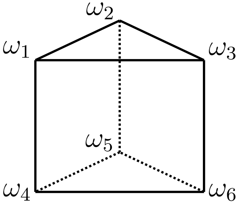
The last two examples show a difference between a quasi-classical structure and a classical system. For example, in the square system, each state is decomposed as , where is a mixture of and and of and . For a given , while is uniquely determined, and are not unique.
To conclude this subsection, we exhibit several properties of quasi-classical structures.
Proposition 3.16.
Let be a state space with and be the set of all its pure states, If there exists a quasi-classical decomposition for , then holds, and the equality is satisfied only if is a simplex with pure states.
Proof.
To prove the first claim, we introduce a set of its elements with each and consider a relation . Applying the corresponding quasi-classical observable , we find that for all , i.e, is a linearly independent set, which implies . To prove the second claim, assume that holds. In this case, we can find that each is composed of only one element. In fact, if we suppose , then can be expressed as with each and (note that such is a basis of due to the assumption ). Then, applying the corresponding quasi-classical observable , we find . Hence the pure states of is given by linearly independent states.
Proposition 3.17.
Let and be a state space and the set of all pure states respectively, and let be a disjoint decomposition for .
The decomposition is quasi-classical if and only if it satisfies the following condition ():
()
if is expressed as , where each with the convex hull of and and probability
distributions on , then holds for all .
The proof of this proposition is given in Appendix C.
3.4 Universal programmings in GPTs
In the previous part, we found that a quasi-classical structure naturally appears in a system when we consider implementing reversible dynamics via a program in an apparatus. In the following, we show that an apparatus with a quasi-classical structure also plays an important role.
Definition 3.18.
Let be an integer with . An apparatus has an -universal programming property if for any with and arbitrary there exist a composite system and such that there are states implementing the reversible dynamics through .
We obtain the following theorem.
Theorem 3.19.
An apparatus has the -universal programming property if and only if has a quasi-classical structure such that with .
The following two lemmas prove the claim.
Lemma 3.20.
Let be an apparatus with a quasi-classical strucutre . For a system with and , one can construct a composite system and a reversible dynamics such that each pure state works as a program implementing its corresponding .
Proof.
Let be a quasi-classical observable corresponding to the quasi-classical decomposition . We employ the minimum tensor product to define . We first note that the composite system also has a quasi-classical structure. In fact, we can see that the set of all its pure states is given by . It has a decomposition
This decomposition is quasi-classical because the observable satisfies for . It follows that each is decomposed as with (). The probability distribution is uniquely determined due to Proposition 3.17. Now we define a map by . This map can be extended safely to an affine bijection . We can further extend this map to the whole by . It is easy to see that holds.
We write a simplex with pure states as : with affinely independent .
Lemma 3.21.
Let be a classical system with pure states, i.e., , and be an apparatus. If for arbitrary reversible dynamics on there exists a reversible dynamics on the composite (remember that holds because is a simplex) through which are implemented, then has a quasi-classical structure with degree .
Proof.
Let be the pure states of . Each reversible dynamics on is described by a permutation of . Let us consider a reversible dynamics on . For any and , a pure state is mapped to . It is expressed as , where are affine maps defined on . Since is pure, there exists (depending on ) such that and for . Operating , we find that holds, where is the dual map for (the Heisenberg picture), that is, with is an observable satisfying either or for . On the other hand, there exists a family of permutations such that for each , and we introduce reversible dynamics by for all . Assume that implements . By the assumption, there exist programs such that holds except for , that is, holds. Therefore, we conclude that has a quasi-classical structure of degree .
We should remember that the degree satisfies and that the equality is attained by a classical system with pure states (see Proposition 3.16).
4 Programming of channels in GPTs
We have so far considered programming reversible dynamics in the framework of GPTs to prove that this is possible only when the apparatus is close to classical theory. In this section, we investigate whether similar observation can be obtained when programming more general state changes, i.e., channels.
4.1 Irreversible universal programming
We start with introducing a similar notion to the one in Definition 3.18.
Definition 4.1.
Let be an integer with . An apparatus has an irreversible -universal programming property if for any with and arbitrary , there exist a composite system and such that there are states implementing distinct channels of through .
Similarly to Theorem 3.19, we obtain the following observation.
Theorem 4.2.
An apparatus has an irreversible -universal programming property if and only if there exists a family of perfectly distinguishable states in .
Remark 4.3.
A similar result to Theorem 4.2 was obtained also in [28]. They both manifest that if we use a set of states as programs to implement arbitrary channels on an arbitrary system via a channel on a total system, then it is necessary and sufficient that the states are perfectly distinguishable. This indication can be compared with our previous result Theorem 3.19, where quasi-classical structures appear as a consequence of considering reversible dynamics instead of channels.
The following two lemmas prove the claim of the theorem.
Lemma 4.4.
Let be a perfectly distinguishable set of states, and be a system with and . One can construct a composite system and a channel such that each state works as a program implementing its corresponding channel .
Proof.
Let be an observable for the perfectly distinguishable such that . We employ the minimum tensor to define . Now we constitute in the following way. First, we define a map by the relation with some and its affine extension, where is a simplex with pure states . We note that this map defines successfully a channel: . Next, we define another map as a measure-and-prepare channel [14] on by the observable and states with the unit effect for and states in . That is, is given by the tensor product of the identity channel on and the corresponding measure-and-prepare channel on , which particuarly satisfies
Finally, we introduce by the tensor product of the identity channel on and the channel on defined via and its affine extension such that . We note that each is not necessarily bijective. It is easy to see that the map given by the composite of the channel and the partial trace implements .
Lemma 4.5.
Let be a classical system with pure states, i.e., . Assume that an apparatus implements arbitrary distinct channels on with programs . Then is perfectly distinguishable.
Proof.
Let be the pure states of . We introduce channels by , where is a family of permutations satisfying for each . Assume that states programs through a channel . We obtain with for each pure state of the system. The term has another expression through maps on . It follows that
or
where is the unit effect on and is the dual map for . We note that holds, i.e., defines an observable on for each . Therefore, if we define an observable with , then it satisfies , i.e., is perfectly distinguishable.
4.2 Approximate programmings via regular polygon theories
In the previous subsection, we demonstrated that channels can be programmed by means of perfectly distinguishable set of states in any GPT. Then it is natural to ask how well one can program them if we use a set of states that are not perfectly distinguishable. In this part, following the argument in Lemma 3.21 and Lemma 4.5, we consider programming channels on a classical system by using pure states of the regular polygon theory [16] with sides as programs, and investigate how well those programs can realize the desired channels.
The state space of the regular polygon theory with sides is given by the convex hull of pure states in with
where . The corresponding effect space is given by
or
| (4.7) |
In this expression, we identify effects with elements in the vector space spanned by the state space through the Riesz representation theorem [29] (thus the action of an effect on a state is given by their inner product). We also note that under this parameterization, holds, i.e., for any , there exists such that .
Let us consider the following game between two parties, Alice and Bob. Alice has a classical system with sufficiently large , and hopes to implement a family of reversible dynamics on . Representing each as through a permutation of , we assume that they satisfy for all and . On the other hand, Bob has a polygon system , and can control the total system, that is, Bob can determine channel on the total system . The game goes as follows: Alice chooses randomly one of the dynamics , and then Bob prepares the corresponding initial state (program) of (see (4.2)). Our question is how well Bob can choose the channel to make the state a good program. To tackle this problem, let us consider the case where Alice’s initial state is . Because
| (4.8) |
holds for all , where are affine maps on , the probability of observing the successful dynamics for this is given by with the dual map for . The average with respect to the initial state is . Since Alice chooses the dynamics randomly, the total success probability is written as
| (4.9) |
Then what we want to obtain is the maximum success probability with respect to every channel on the total system implementing by Bob, that is,
| (4.10) |
To evaluate (4.9), we focus on the expression (4.8). We can find that the maps satisfy for all . Thus defines a family of observables , where each observable is given by by means of the dual maps for . On the other hand, for a given family of observables with , one can construct such that for all . In fact, if we set with an arbitrary state for each , then the map defined through the expression (4.8) is a channel on and satisfies the condition for all . It follows that the maximization over all channels in (4.10) can be replaced by the maximization over all families of observables on with outcomes. Now (4.10) becomes
where is the set of all observables on with outcomes and is its products. Because is assumed, the above equation can be rewritten as
| (4.11) |
We note that the last equation is obtained by identifying an observable with outcomes with observable with outcomes.
The problem is to search how well we can optimize (4.11), that is, to find an observable that maximizes (4.11). This problem is equivalent to the so-called state discrimination problem, and there have been studies on this problem not only in quantum theory [30] but also in GPTs [31, 32, 33, 34]. Here we refer to the results in [31] by Kimura et al. According to their results, if we can find a set of states and positive numbers with each (called a “weak Helstrom family”) for such that
| (4.12) |
and
| (4.13) |
for all , then holds. They also revealed that the equality holds if the observable satisfies for all . In the regular polygon theory , we can easily find a weak Helstrom family for . In fact, if we set
| (4.14) |
then it is easy to see that they satisfy (4.12) and (4.13). Moreover, we can find that the condition is satisfied with each given by (remember (4.2) and (4.7))
| (4.15) |
We note that the coefficients and are determined so that holds. This is realized by a channel satisfying
where the linear operator on is defined as with the Euclidean inner product on . For this , the probability (4.9) attains its maximum value as
| (4.16) |
We can see, for example, that , and . The above result (4.16) is compared with the success probability to program reversible dynamics on the system by a single bit (thus the total system is ). Since has two pure states, it can program perfectly at most two reversible dynamics on . It follows that in this case the optimal value of average success probability is . This manifests that when implementing reversible dynamics on a classical system, using the regular polygon theory as apparatus with sides results in a better or equal success probability than using classical bit.
5 Conclusion
In this study, we considered the generalization of quantum programming scheme to GPTs. It was found that a family of reversible dynamics on a target system is programmable only if a pairwise distinguishable set of states in an apparatus is used as programs. While this result seems to be just a straightforward generalization of the quantum result, it should be emphasized that this was obtained for any physically valid composite of the system and apparatus, i.e., any bipartite state space between the minimal and the maximal tensor products of them. On the other hand, we also considered changing the programming scenario itself: universal programming of reversible dynamics and channels, and investigated when an apparatus makes them possible. It was demonstrated that the former scheme is realizable if and only if the apparatus has a quasi-classical structure, which was originally derived for the target system in the initial programming scheme, and that the latter is possible if and only if the corresponding programs in the apparatus are perfectly distinguishable. We believe that the former result is particularly important in that it is peculiar to GPTs beyond quantum theory. We also presented numerical evaluations for how well we can implement channels on a classical system if states in regular polygon theories (that are in general not perfectly distinguishable) are used as programs, where only approximate programming is possible. It will be interesting to present similar evaluations for more general cases when channels on non-classical GPTs are to be programmed. Future study will be also needed to give further investigations of quasi-classical structures. As Example 3.15 shows, state spaces with quasi-classical substructures seem to have properties that the classical (triangle) and square theories have. Since these two theories exhibit respectively minimum and maximum values for the CHSH value [8, 35] or incompatibility [36], it may be possible to give other theoretical characterizations for quasi-classical structures.
Acknowledgment
The authors thank Yui Kuramochi for helpful suggestions. TM acknowledges financial support from JSPS (KAKENHI Grant No. JP20K03732). RT acknowledges financial support from JSPS (KAKENHI Grant No. JP21J10096).
Appendix Appendix A A pairwise distinguishable family of states is always finite.
In this appendix, we prove that a pairwise distinguishable family of states in a finite-dimensional state space is a finite set.
Proposition A.1.
Let be a state space in with , and let be a pairwise distinguishable set of states. Then is a finite set, i.e., .
Proof.
Since , we can choose a linearly independent set of states that forms a basis of . Then a set of linear functions on defined as can be introduced. It can be seen that is a linearly independent set of vectors, and thus forms a basis of the dual space . For such vectors, we define and . We note that and are finite quantities because is a compact set. Now we divide the interval into parts as . It defines a pairwise disjoint partition of by
where . In other words, a state satisfies for each . Let us suppose that the set is an infinite set. Because is infinite, there exists at least one such that is an infinite set ( is enough for the following argument). For such , we take its elements . Since are perfectly distinguishable, there exists an effect such that and holds. On the other hand, representing in terms of the basis as , we have for each because holds. It follows that
but, because we can choose arbitrarily large , it contradicts.
Appendix Appendix B distinct states can be discriminated by an -outcome observable via the observed statistics
In this appendix, we prove that distinct states can be discriminated by an observable with outcomes in terms of the observed probability distributions.
Proposition B.1.
Let be a state space in with , and let be a finite set of distinct states. There exists an observable with outcomes such that the observed probability distributions are all distinct.
Proof.
Let be a subspace of , and let be its dimension. Then there exists a linearly independent set . Also, there is a linearly independent set of states such that forms a basis of . We introduce a set of elements of defined as , which is a basis of . It can be seen easily that the unit effect for is represented as . Now we construct an -outcome observable that discriminates states in . Let be a set of elements in defined as
We note that holds. The vectors discriminates states in . In fact, if states satisfy for all , then, representing the states as and via the basis of , we obtain for all , that is, . Let . We have for all and . In addition, the vectors discriminate states in because the condition is equivalent to whenever . Then we take a suitable normalization for to obtain an observable that discriminates states in (remember that holds). Adding the zero effect to if necessary, we have an -outcome observable that discriminates states in .
Remark B.2.
From the above proof, we obtain the following observation: for a state space , there exist observables with at most outcomes such that an arbitrary number of distinct states can be discriminated through the probability distributions observed in their measurements. Those observables are called informationally complete observables [37, 38], and informationally complete observables with outcomes (i.e. observables whose effects compose a basis of ) are called particularly minimal informationally complete observables [6].
Appendix Appendix C Proof of Proposition 3.17
In this appendix, we present the proof of Proposition 3.17 shown as follows.
Proposition 3.17.
Let and be a state space and the set of all pure states respectively, and let be a disjoint decomposition for .
The decomposition is quasi-classical if and only if it satisfies the following condition ():
()
if is expressed as , where each with the convex hull of and and probability
distributions on , then holds for all .
Proof.
(the ‘only if’ part)
Due to the Krein-Milman theorem [29], any can be
decomposed as
, where
and is a probability distribution.
We introduce
and
for satisfying to obtain
.
To prove the uniqueness of , suppose that there are two decomposition
with .
Applying the quasi-classical observable associated with the quasi-classical decomposition, we obtain
for each .
(the ‘if’ part)
The claim is proved by induction on the integer .
First we consider the case of , i.e., .
For the corresponding decomposition , it holds that .
To see this, suppose that and .
There exist positive numbers , , , and , and pure states , , , and such that
| (C.1) | ||||
| (C.2) |
It follows that
or
where . Because
hold, we have from the assumption
This contradicts (C.1), and thus is concluded. Then, according to the separating hyperplane theorem (Theorem 11.2 in [39]), there exist hyperplanes and in such that , , and (in particular, and are parallel). They can be represented as and as and respectively, where with and , and is an inner product in . We note that we identify the dual space with via the inner product in the following. We can observe that the vector , where is the unit effect, satisfies
| (C.3) |
In particular, is properly an effect because for all due to (C.3), and thus is quasi-classical ( gives the corresponding quasi-classical observable).
Assume that the claim holds when , and consider the decomposition with satisfying the relevant condition . Expressing , we introduce the disjoint decomposition , where
It is not difficult to see that this decomposition satisfies , and thus there exists a quasi-classical observable such that
On the other hand, if we consider the disjoint decomposition , where
then there similarly exists an observable such that
Now we obtain easily for . Besides, we can observe that is a proper effect satisfying
Therefore, a family of effects defined as
is an observable that satisfies
that is, the initially considered decomposition is quasi-classical.
References
- [1] M. A. Nielsen and I. L. Chuang, Quantum Computation and Quantum Information: 10th Anniversary Edition. Cambridge University Press, 2010.
- [2] M. A. Nielsen and I. L. Chuang, “Programmable quantum gate arrays,” Physical Review Letters, vol. 79, pp. 321–324, July 1997.
- [3] Y. Yang, R. Renner, and G. Chiribella, “Optimal universal programming of unitary gates,” Physical Review Letters, vol. 125, p. 210501, Nov. 2020.
- [4] T. Heinosaari, T. Miyadera, and M. Tukiainen, “Limitations on post-processing assisted quantum programming,” Quantum Information Processing, vol. 16, p. 85, Feb. 2017.
- [5] L. Hardy, “Quantum theory from five reasonable axioms,” 2001, arXiv:quant-ph/0101012.
- [6] H. Barnum, J. Barrett, M. Leifer, and A. Wilce, “Cloning and broadcasting in generic probabilistic theories,” 2006, arXiv:quant-ph/0611295.
- [7] H. Barnum, J. Barrett, M. Leifer, and A. Wilce, “Generalized no-broadcasting theorem,” Physical Review Letters, vol. 99, p. 240501, Dec. 2007.
- [8] J. Barrett, “Information processing in generalized probabilistic theories,” Physical Review A, vol. 75, p. 032304, Mar. 2007.
- [9] G. Chiribella, G. M. D’Ariano, and P. Perinotti, “Probabilistic theories with purification,” Physical Review A, vol. 81, p. 062348, June 2010.
- [10] G. Chiribella, G. M. D’Ariano, and P. Perinotti, “Informational derivation of quantum theory,” Physical Review A, vol. 84, p. 012311, July 2011.
- [11] L. Masanes and M. P. Müller, “A derivation of quantum theory from physical requirements,” New Journal of Physics, vol. 13, p. 063001, June 2011.
- [12] H. Barnum, J. Barrett, M. Leifer, and A. Wilce, “Teleportation in general probabilistic theories,” in Proceedings of Symposia in Applied Mathematics, vol. 71, pp. 25–48, 2012.
- [13] L. Lami, Non-classical correlations in quantum mechanics and beyond. PhD thesis, Universitat Autònoma de Barcelona, 2017.
- [14] M. Plávala, “General probabilistic theories: An introduction,” 2021, arXiv:2103.07469.
- [15] R. Takakura, Convexity and uncertainty in operational quantum foundations. PhD thesis, Kyoto University, 2022.
- [16] P. Janotta, C. Gogolin, J. Barrett, and N. Brunner, “Limits on nonlocal correlations from the structure of the local state space,” New Journal of Physics, vol. 13, no. 6, p. 063024, 2011.
- [17] P. Janotta and R. Lal, “Generalized probabilistic theories without the no-restriction hypothesis,” Physical Review A, vol. 87, p. 052131, May 2013.
- [18] N. Brunner, M. Kaplan, A. Leverrier, and P. Skrzypczyk, “Dimension of physical systems, information processing, and thermodynamics,” New Journal of Physics, vol. 16, p. 123050, Dec. 2014.
- [19] P. Busch, P. J. Lahti, J.-P. Pellonpää, and K. Ylinen, Quantum Measurement. Theoretical and Mathematical Physics, Springer International Publishing, 2016.
- [20] T. Heinosaari and M. Ziman, The Mathematical Language of Quantum Theory: From Uncertainty to Entanglement. Cambridge: Cambridge University Press, 2011.
- [21] G. Aubrun, L. Lami, C. Palazuelos, and M. Plávala, “Entangleability of cones,” Geometric and Functional Analysis, vol. 31, pp. 181–205, May 2021.
- [22] C. Zander and A. R. Plastino, “Fidelity measure and conservation of information in general probabilistic theories,” EPL (Europhysics Letters), vol. 86, p. 18004, Apr. 2009.
- [23] G. Kimura, K. Nuida, and H. Imai, “Distinguishability measures and entropies for general probabilistic theories,” Reports on Mathematical Physics, vol. 66, no. 2, pp. 175 – 206, 2010.
- [24] I. Namioka and R. R. Phelps, “Tensor products of compact convex sets,” Pacific Journal of Mathematics, vol. 31, no. 2, pp. 469 – 480, 1969.
- [25] R. Takakura and T. Miyadera, “Preparation uncertainty implies measurement uncertainty in a class of generalized probabilistic theories,” Journal of Mathematical Physics, vol. 61, no. 8, p. 082203, 2020.
- [26] Z. Wu, C. Zhu, and X. Zhang, “Measurement interpretation and information measures in general probabilistic theory,” Central European Journal of Physics, vol. 11, pp. 317–324, Feb. 2013.
- [27] T. M. Cover and J. A. Thomas, Elements of Information Theory. Hoboken, New Jersey: John Wiley & Sons, Inc., 2nd ed., 2006.
- [28] G. Chiribella, “Distinguishability and copiability of programs in general process theories,” International Journal of Software and Informatics, vol. 8, no. 3-4, p. 209, 2014.
- [29] J. B. Conway, A Course in Functional Analysis, vol. 96 of Graduate Texts in Mathematics. Springer-Verlag New York, 1st ed., 1985.
- [30] J. Bae and L.-C. Kwek, “Quantum state discrimination and its applications,” Journal of Physics A: Mathematical and Theoretical, vol. 48, p. 083001, Jan. 2015.
- [31] G. Kimura, T. Miyadera, and H. Imai, “Optimal state discrimination in general probabilistic theories,” Phys. Rev. A, vol. 79, p. 062306, Jun 2009.
- [32] J. Bae, D.-G. Kim, and L.-C. Kwek, “Structure of optimal state discrimination in generalized probabilistic theories,” Entropy, vol. 18, no. 2, 2016.
- [33] R. Takagi and B. Regula, “General resource theories in quantum mechanics and beyond: Operational characterization via discrimination tasks,” Phys. Rev. X, vol. 9, p. 031053, Sept. 2019.
- [34] Y. Yoshida, H. Arai, and M. Hayashi, “Perfect discrimination in approximate quantum theory of general probabilistic theories,” Phys. Rev. Lett., vol. 125, p. 150402, Oct. 2020.
- [35] S. Popescu and D. Rohrlich, “Quantum nonlocality as an axiom,” Foundations of Physics, vol. 24, pp. 379–385, 1994.
- [36] A. Jenčová and M. Plávala, “Conditions on the existence of maximally incompatible two-outcome measurements in general probabilistic theory,” Physical Review A, vol. 96, p. 022113, Aug. 2017.
- [37] P. Busch, “Informationally complete sets of physical quantities,” International Journal of Theoretical Physics, vol. 30, pp. 1217–1227, Sept. 1991.
- [38] M. Singer and W. Stulpe, “Phase‐space representations of general statistical physical theories,” Journal of Mathematical Physics, vol. 33, no. 1, pp. 131–142, 1992, https://doi.org/10.1063/1.529975.
- [39] R. T. Rockafellar, Convex Analysis, vol. 28 of Princeton Mathematical Series. Princeton University Press, 1970.