Automating In-Network Machine Learning
Abstract.
Using programmable network devices to aid in-network machine learning has been the focus of significant research. However, most of the research was of a limited scope, providing a proof of concept or describing a closed-source algorithm. To date, no general solution has been provided for mapping machine learning algorithms to programmable network devices. In this paper, we present Planter, an open-source, modular framework for mapping trained machine learning models to programmable devices. Planter supports a wide range of machine learning models, multiple targets and can be easily extended. The evaluation of Planter compares different mapping approaches, and demonstrates the feasibility, performance, and resource efficiency for applications such as anomaly detection, financial transactions, and quality of experience. The results show that Planter-based in-network machine learning algorithms can run at line rate, have a negligible effect on latency, coexist with standard switching functionality, and have no or minor accuracy trade-offs.
1. Introduction
The rapid growth of data volume and the increasingly heavy demands for data exploitation are creating an ever-increasing processing burden on computing systems (Zhang et al. 2017). Concerns about a future shortage of computing resources drove the networking community to consider the underused processing resources within the network (Sanvito et al. 2018; Xiong and Zilberman 2019). Programmability within the network has been promoted by the emergence of programmable network devices (Feamster et al. 2014; Bosshart et al. 2013). These potential computing resources in the network boost performance, while at the same time increasing power efficiency (Tokusashi et al. 2019).
Building upon the programmability of network devices and their high packet processing rate, in-network computing was demonstrated to improve a range of applications, from network services and monitoring (Katta et al. 2016; MacDavid et al. 2021; Ben Basat et al. 2020; Kim et al. 2016; Bhamare et al. 2019) to caching and consensus (Jin et al. 2017; Dang et al. 2020). These computing tasks require low latency, high throughput and power efficiency, while at the same time flooding the network with data exchanges. As such, in-network computing was suggested as a means to improve machine learning (ML) performance, both in the acceleration of traditional host-based ML training using in-network aggregation (Sapio et al. 2021; Lao et al. 2021), and ML inference by using in-network ML (Sanvito et al. 2018; Xiong and Zilberman 2019; Zheng et al. 2022). In-network ML is advantaged by its deployment location, illustrated in Figure 1, enabling latency benefits and high throughput. Unlike server-based traditional ML, it does not introduce additional traffic into the network.

Researchers have so far demonstrated the offloading of algorithms such as Support Vector Machines (SVM)11 1 Appendix A provides a list of all acronyms used in this paper. (Xiong and Zilberman 2019; Swamy et al. 2020; Zheng et al. 2022), Naïve Bayes (NB) (Xiong and Zilberman 2019; Zheng et al. 2022), K-means (KM) (Xiong and Zilberman 2019; Friedman et al. 2021; Swamy et al. 2020; Zheng et al. 2022), Decision Trees (DT) (Zheng and Zilberman 2021; Xiong and Zilberman 2019; Zheng et al. 2022), Random Forest (RF) (Zheng and Zilberman 2021; Lee and Singh 2020; Busse-Grawitz et al. 2019; Xavier et al. 2021; Zhang et al. 2021; Zheng et al. 2022), and (Binary) Neural Networks (NN) (Sanvito et al. 2018; Zhong et al. 2021; Siracusano et al. 2018; Swamy et al. 2020; Siracusano and Bifulco 2018; Siracusano et al. 2020; Qin et al. 2020). These works have provided proofs-of-concept and laid the foundation of in-network ML. However, despite five years of research towards in-network ML, most of the works remained as preliminary implementations, or had prohibitive limitations such as limited model type, size and complexity, compromised accuracy, and lack of comparison to other alternatives.
Previous in-network ML works have used a wide range of targets, architectures, and mapping procedures. This makes it difficult to reproduce or extend the state-of-the-art, thereby hindering the development and adoption of in-network ML. To that end, a framework that integrates the development and evaluation of commonly-used in-network ML models is needed.
In this paper, we present Planter, a framework for plug-and-play in-network ML development and deployment. Plant-er supports a range of ML models (e.g., SVM, XGB, BNN, PCA), multiple architectures (PSA (Group 2017), TNA (Intel 2021), v1model (Peterson et al. 2021)), multiple targets (Tofino (Gurevich and Fingerhut 2021), P4Pi (Laki et al. 2021) & BMv2 (Consortium 2020a)), and several use cases (e.g., attack detection, financial transactions). Planter is a modular and scalable solution, enabling support for future in-network classification models and use cases. It also enables a comparison between different ML mapping methods.
The main contributions of this paper are:
- •
Introducing Planter, a modular framework for streamlined deployment of different in-network ML algorithms across multiple architectures and targets. Plant-er’s modular design enables easily adding new models, targets, architectures, and features.
- •
Generalizing, and implementing a wide range of state-of-the-art in-network ML algorithms, upgrading several previous in-network ML implementations, and proposing multiple new in-network ML algorithms mappings.
- •
Evaluating and comparing state-of-the-art and newly proposed in-network ML algorithms in terms of functionality, resources, scalability, and throughput. The comparison results can be used as a selection and referencing guidelines for future in-network ML research.
2. Background
This section provides the background and the motivation for Planter, as well as setting guidelines for its design.
Programmable Network Devices
The introduction of programmable network devices has enabled users to create customizable data planes. This was further driven by the introduction of the P4 programming language(Bosshart et al. 2014) and the RMT architecture (Bosshart et al. 2013). Today, programmable data planes are supported on a range of hardware and software targets, using different architectures (PSA (Group 2017), TNA (Intel 2021), v1model (Peterson et al. 2021), and others).
In-network ML
This paper defines in-network ML as the partial or full offloading of ML algorithms to run within network devices. In this work, we limit the scope to the forward classification process of ML algorithms being offloaded to the data plane, while the training part remains on the host (including accelerators) or in the control plane. In-network ML algorithms follow an offline training, online (in-band) inference pattern. Feature extraction can be done either by parsing within the data plane or customized headers. A mapped ML model is typically implemented within the Match/Action (M/A) pipeline, and the decision can be stored in a header or turned to an action within the network device. In-network aggregation (Sapio et al. 2021; Lao et al. 2021) is outside this scope.
2.1. Motivation
In network deployments, programmable network devices provide primarily switching and routing-support functions. These functions require a significant portion of the programmable devices’ resources, but often don’t exhaust them, as demonstrated by Tofino’s switch.p4. In-network ML tasks can utilize remaining resources, co-existing with mandatory and traditional switch functions (see §7.3).
Several use cases are commonly tied with ML for networking, and are applicable to in-network ML too:
Traffic Engineering
The use of ML to improve traffic engineering can allow reducing communication overheads between cloud and edge (Paolucci et al. 2019; Paolucci et al. 2021), improve heavy hitter detection (Zhang et al. 2021) and quality of experience (QoE) prediction (Wassermann et al. 2020), and support IoT classification at line-rate (Xiong and Zilberman 2019).
Anomaly Detection
An important use case of in-network computing and in-network ML is network security (Xavier et al. 2021; Lee and Singh 2020; Consortium 2020b), allowing early detection and fast mitigation of attacks, potentially preventing distributed attacks.
Financial Transactions
ML models are widely used to perform financial tasks, and stock market forecasting is a significant one of them (Choudhry and Garg 2008; Shen et al. 2012; Leung et al. 2014; Henrique et al. 2018). In the meanwhile, hardware and software solutions are designed for accelerating the development of financial applications (Leber et al. 2011; Lockwood et al. 2012). In a field where every nanosecond counts, the two-fold goal is to increase prediction accuracy, while minimizing latency.
2.2. State-of-the-Art In-Network ML
The in-network ML algorithms realized to date can be divided into three categories: tree-based models (including decision trees and ensemble models), BNN-based models, and other classic ML models.
Work ML Models Targets PC2 MS2 SC2 PP2 SwitchTree (Lee and Singh 2020) RF BMv2 ✗ ✗ P ✗ pForest (Busse-Grawitz et al. 2019) RF Tofino, BMv2 ✗ ✗ ✗ ✗ IIsy (Xiong and Zilberman 2019; Zheng et al. 2022) SVM, KM, DT NetFPGA-SUME ✗ ✓ ✓ ✗ NB BMv2 Clustream (Friedman et al. 2021) KM Spectrum-3 ✗ ✗ ✗ ✗ toNIC (Siracusano et al. 2018) NN NFP4000 ✗ ✗ ✗ ✗ BaNaNa (Sanvito et al. 2018) NN RMT-NIC ✗ ✗ ✗ ✗ N3IC (Siracusano et al. 2020) NN NetFPGA-SUME ✗ ✗ ✗ ✗ Qin (Qin et al. 2020) NN Agilio CX, BMv2 ✗ ✗ P ✗ Planter1 SVM, KM, DT Tofino, BMv2 ✓ ✓ ✓ ✓ XGB, RF, NB P4Pi-BMv2 NN, PCA, AE P4Pi-T4P4S IF, KNN 1 Planter builds upon IIsy (Xiong and Zilberman 2019; Zheng et al. 2022), which supports NetFPGA-SUME. However, as SUME is EoL, Planter currently does not support it. 2 PC - Peer Comparison Provided, MS - Multiple Solutions Provided, SC - Source Code Available, PP - Plug-and-Play Ability Enabled.

Table 1 presents a partial snapshot of recent in-network ML works, with more works discussed in this section. Two types of solutions have been presented to tree-based models. The first type, presented in IIsy (Xiong and Zilberman 2019; Zheng et al. 2022) is referred to in this paper as an encode-based (EB) solution (see §4.1). This solution was also implemented in (Xavier et al. 2021). The second type, used by pForest and SwitchTree (Busse-Grawitz et al. 2019; Lee and Singh 2020), is direct-mapping (DM) (§4.3). BNN-based models are mainly based on the XNOR Net(Rastegari et al. 2016). With the help of XNOR operations and Hamming Weight (Pop count), Siracusano (Sanvito et al. 2018; Siracusano et al. 2020; Siracusano and Bifulco 2018; Siracusano et al. 2018; Siracusano et al. 2022) and Qin (Qin et al. 2020) realized binarized Multiple Layer Perceptron (MLP) in the data plane. They mainly targeted SmartNICs, which have less rigid limitations than switch ASIC. Other traditional ML models, including SVM, NB, and KM, were introduced by IIsy (xiong2019switches.zheng2022iisy), with multiple mappings per model. However, the implementations are FPGA-based and are not resource optimized. Clustreams (Friedman et al. 2021) suggested a different KM mapping of IIsy’s. Taurus (Swamy et al. 2020) and IOI (Zhong et al. 2021) use modified ASIC to realize complex operations, and are outside the scope of this paper.
2.3. The Gap in In-Network ML
Although the development of in-network ML solutions is promising, a gap remains between a functional prototype and a plug-and-play solution on commodity devices. As shown in Table 1, most of the existing in-network ML works support only one type of ML model and one type of a target, typically a SmartNIC or a software switch. A proposed algorithm has only one model mapping solution (in most cases) and is not compared with other in-network ML solutions. Moreover, many solutions have no publicly available source code. Where an artifact was published (Qin et al. 2020; Xiong and Zilberman 2019), only P4 code is available. Aspects such as weight transformers are missing, and a lot of manual changes are needed when updating a model.
These aforementioned limitations can be divided into four groups of challenges: high reproduction difficulty, limited model and target options, limited model size, and limited comparison.
2.4. Planter Design Guidelines
Planter aims to narrow the gap in production in-network ML, and sets the following design guidelines:
Ease of use. Mapping ML models to programmable network devices using P4 is not trivial. New targets, architectures, and models may result in significant changes in (i) trained models, (ii) P4 programs, (iii) mapped model parameters to M/A tables or registers, and (iv) table loading process. An easy-to-operate in-network ML end-to-end solution is needed to handle the process and flexibly adapt to changes (§3.1).
Optimized models. Programmable network devices are primarily designed for packet processing and forwarding. They have limited memory and stages, and support a constrained set of mathematical operations and data types. Map-ped ML algorithms need to trade off model size and performance to fit on a network device. Thus, the framework should support a wide range of predefined and optimized ML models. The resource overhead of the mapped ML algorithms should be minimized as not to affect mandatory network functionality (§4).
Modularity. ML algorithms are emerging rapidly. New architectures and software/hardware targets are reaching the market. The framework should be able to support new ML algorithms, architectures, and targets. It should be easy to update application scenarios. This calls for a modular design with elements easily added, updated, or replaced, independent of other framework components (§3.2 - §5).
3. Planter Framework
Planter is a framework for offloading ML models into programmable network devices. The framework uses configuration files to identify the chosen ML model, architecture, target, dataset, and use case. It automatically generates, compiles, loads, and runs the mapped ML models on the target.
3.1. Workflow and Main Components
The workflow of Planter, shown in Figure 2, has seven steps. In the first two steps, Planter loads a dataset ❶ and trains it ❷. The model is mapped to P4 ❸, using the selected architecture and target. Generated P4 code is compiled ❹ and loaded to the data plane target ❺. In step ❻, table entries and registers are loaded through the control plane. In the final step ❼, the auto generated testing module runs a functionality test on the target.
The generated data plane, shown in Figure 2 ![[Uncaptioned image]](2205.08824v1/c_A.png) , has three functional parts: standard switching functionality, feature extraction for ML models, and ML inference. The ML feature extraction and inference can be parallel to the standard functionality (parser operation is merged).
, has three functional parts: standard switching functionality, feature extraction for ML models, and ML inference. The ML feature extraction and inference can be parallel to the standard functionality (parser operation is merged).
The workflow is realized using five components: Input Configurations, Data Loader, Model Trainer & Converter, P4 Generator, and Model Compiler & Tester. The detailed design of each component is described next.
Input configurations
Planter is using configuration files to drive its one-click operation. The configurations can be loaded from a file, or entered through an interactive CLI.
Data Loader
The data loader loads datasets for training purposes. It is use-case specific, based on used features and data format. All loaded data are stored in the same format.
Model Trainer & Converter
ML Training is conducted by the Model Trainer, which drives a standard training framework. Trained models are next mapped to the M/A pipeline in the Model Converter. A software test is generated to test the validity of the mapped model.
P4 Generator
There are three parts to the P4 Generator. The Standard P4 Generator contains architecture-specific P4 code and is the main program that integrates the other P4 codes. This is where the standard network functionality resides. The Common P4 Generator contains the use case specific P4 code, such as bespoke feature extraction. The Dedicated P4 Generator creates the model-related P4 code.
Model Compiler & Tester
The Model Compiler & Tester are deployed in the control plane. The Model Compiler generates bash scripts to compile, load, and run mapped ML models. The Tester generates testing scripts and runs the functionality test on the selected target.
3.2. Modular Framework Design
Planter is a modular framework. Modules are independent and can be flexibly and easily replaced. The framework supports many ML models, architecture models, target modules, and use case modules. For navigation simplicity, modules are arranged in folders by type. This can be rearranged by users. In addition to the above, Planter provides a set of common functions, such as exact-to-LPM table conversion, which can be used by other modules. More details are provided in Appendix B.
4. ML Models in Planter
This section provides a detailed look into the Model Trainer & Converter component (Figure 2 step ❷). Planter supports a range of in-network ML algorithms, e.g., SVM, NB, DT, RF, XGB, IF, KM, KNN, and NN. Among these implemented algorithms, Planter also upgrades some previously proposed implementations (e.g., DT, RF, and NB), and supports new ML algorithms (e.g., XGB, IF, KNN, AE, and PCA). The modularity of the framework allows future support in Planter of other types of in-network algorithms, as well as other enhancements.
Types SVM DT RF XGB IF NB KM KNN PCA AE NN EB ✧3 ✧3 ✧ ✧2 ✓ ✧ LB ✓3 ✧2 ✓3 ✧ ✧ DM ✓ ✓ ✓
In Planter, ML algorithms mapping can be classified into three types: encode-based (EB), lookup-based (LB), and direct-mapping (DM). Table 2 shows all the ML models supported under these three approaches. EB solutions encode the feature space for algorithms based on input feature space partitioning. LB solutions are based on lookup in tables of intermediate results. DM approaches map the model directly into the pipeline, using alternative operations or result approximation. This section introduces the details of one variation of each model. All variations’ implementations can be found in Planter’s repository (Zheng 2022).
4.1. Encode-Based Solutions
Classification algorithms essentially aim to find borders in a feature space, either the original or a mapped one. The area confined by a set of borders (partitions) is labeled as a class. Algorithms use different methods to define their borders. Some use complex functions, while others use linear functions for approximation. EB solutions mainly use linear borders to slice the feature space with codes representing each part of the area in the space.
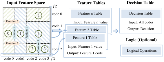

To describe the mapping of a general EB model, consider the input features. To slice input features into classes, a typical method uses feature tables and a decision table. As shown in Figure 3, based on a well-trained model, feature space (e.g., two-dimensional space) is sliced into 6 areas (i.e., area ![[Uncaptioned image]](2205.08824v1/00.png) to area
to area ![[Uncaptioned image]](2205.08824v1/05.png) ) by 5 partitions (i.e., partition
) by 5 partitions (i.e., partition ![[Uncaptioned image]](2205.08824v1/p1.png) to partition
to partition ![[Uncaptioned image]](2205.08824v1/p5.png) ). To map this ML model to M/A pipeline, this input feature space uses two feature tables to record the mapping from feature values to codes, where codes of features represent each area (e.g., area
). To map this ML model to M/A pipeline, this input feature space uses two feature tables to record the mapping from feature values to codes, where codes of features represent each area (e.g., area ![[Uncaptioned image]](2205.08824v1/03.png) coded as: f1-code 3 & f2-code 2). The model stores the mapping from codes to labels in a decision (code) table. Similarly, for the case of dimensional feature space, the model needs feature tables and 1 decision table. Based on this general method, EB solutions vary depending on how algorithms split the feature space.
coded as: f1-code 3 & f2-code 2). The model stores the mapping from codes to labels in a decision (code) table. Similarly, for the case of dimensional feature space, the model needs feature tables and 1 decision table. Based on this general method, EB solutions vary depending on how algorithms split the feature space.
4.1.1. Decision Tree (DT)
DT uses a top-down decision process, and it splits the feature space at each branch (node) until reaching the leaf nodes (Wu et al. 2008). Figure 5 shows a sample DT model and a two-dimensional input feature space split by its branches.

The similarity between Figures 3 and 5 shows that a DT model fits the general EB solution. For any features input space, an encode-based DT (DTEB) requires feature tables, encoding each feature value. The encoded feature space is mapped using a decision table to labels. All feature tables share a pipeline stage (within target limitations) and the entire mapping requires only two logical stages.
In order to generate features tables and decision tables from a trained model, as shown in Figure 4 (illustrating Tree 2 generation process), there are four steps. The process starts with an input of a trained DT. In the step titled “Find feature splits”, the algorithm collects all the branches related to each feature. Then, feature values are encoded (mapping area to a code word) and saved as feature tables in the step “Generate feature table”. The encoding is according to the splitting conditions of the branches. The algorithm next looks at each leaf node and determines which part of the feature space belongs to the node and what range of values it includes. Finally, the step “Generates the tree (also named as code or decision) table” links the mapping from these leaf nodes to the codes pointing to their pieces.
Different from IIsy’s (Xiong and Zilberman 2019) implementation, the DTEB model uses Ternary match in all feature tables, and uses default actions in a tree table to store the most common label. These improvements can significantly reduce the number of table entries stored in the M/A pipeline, and they are applied in all of Planter’s EB ensemble models.
4.1.2. Random Forest (RF)
RF is an ensemble model built from a set of DT models (Ho 1995). The EB RF (RFEB) encodes the trees in parallel and concludes the label by a voting table. In the voting table, the RFEB model groups the results of all DTEB constructing the forest as votes in the forward process. Different from the DT model, a key challenge in the RF mapping is looking up multiple trees in parallel. Figure 4 shows the RF workflow and a toy example of how to map a two-tree RF model to M/A format. For larger models with feature input and -tree models, the mapped M/A model uses feature tables and code tables. Every feature table stores as actions the codes for all trees. In the final stage of the model, voting table are used instead of logic, ao all feature tables and all tree tables are theoretically able to share one logical stage respectively.
4.1.3. XGBoost
XGBoost (XGB) is another type of an ensemble model based on DT. One of the primary differences between XGB and RF is in the value stored at each leaf node. XGB accumulates probabilities from each tree’s leaf nodes to make the final decision (Chen and Guestrin 2016). Due to the operation limitation in some types of programmable devices, it is hard to calculate probablities within the M/A pipeline. To address this issue, the EB XGB (XGBEB) encodes all probabilities in each tree. Then, to create the decision (codes-to-label) table, the XGB mapping workflow calculate all combinations of codes and their cumulative probabilities as well as their final label. The probabilities addition and comparison operation thus can be replaced by simple codes-to-label look-ups in the final decision process.
4.1.4. Isolation Forest
Isolation Forest (IF) is an unsupervised ensemble model based on RF (Liu et al. 2008). To make the decision, the total number of branches used in the forest decision is compared to an anomaly threshold, as shown Equation 1, where is the input instance, is the path length, is the total number of training instance, and is the average of a collection of trees.
| (1) |
EB IF (IFEB) uses a similar method to XGBEB to build the M/A pipeline. The main difference between IFEB and XGBEB is in the M/A table generation process on top of Equation 1.
4.1.5. K-means

The EB KM (KMEB) labels the input based on the distance between the data point and each centroid (Fix and Hodges 1989). The input feature space thus can be divided into small pieces. Figure 6 shows a KMEB toy example in Planter, based on Clustream’s (Friedman et al. 2021) solution, which encodes the feature space (2 dimensional) by using the Quadtree. In the higher dimensional feature space, at each depth of the tree, the input dimensional feature space is divided and labeled into equal parts with the same order. The KMEB requires bits code to represent each area when the maximum depth is . The feature space is split continuously until the tree reaches the maximum depth or all vertices of the current unit belong to one class. According to its tree-like splitting approach, all these codes are stored in the ternary tables. Compared with the EB tree models, the KMEB requires preprocessing before inference.
4.1.6. K-nearest Neighbors
The K-nearest Neighbor (KNN) method splits the feature space in a similar way to KM. The difference is that KNN uses the distance between the vertices and nearest neighbors instead of the centroid.
4.2. Lookup-Based Solutions
Many ML algorithms involve complex mathematical operations between input features and the final logic. These mathematical operations are commonly too complex to implement in the data plane. Lookup-based solutions use M/A tables to store the intermediate results of these operations and thus are able to realize in-network ML in the data plane.

Any ML algorithms with a Decision Process can use the LB solutions as shown in Figure 7. In LB solutions, feature tables store the mapping between each input feature value and intermediate results. These intermediate values then do the remaining basic mathematical operations, typically addition, as the final stage logic. Multiplication operations between middle results are not performed in the final stage logic, and are only supported through lookup tables.
4.2.1. Support Vector Machine (SVM)
SVM maps inputs to hyperplanes, and uses hyperplanes to separate pairs of classes. For a classification task, SVM model requires hyperplanes. Each hyperplane is equivalent to a vote. The final vote can be determined by counting the votes from all hyperplanes and using logic or a decision table (Cortes and Vapnik 1995).
| (2) |
For LB SVM (SVMLB), IIsy (Xiong and Zilberman 2019) proposed three similar solutions by storing the intermediate result of each hyperplane. The solutions are mainly differentiated by the stored intermediate results. Planter realizes the solution that has the most similar structure with the general solution in Figure 7 and with the best scalability, by using feature tables to store the related middle results from all hyperplanes (e.g., Input: , Output ). Each feature table belongs to a logical stage and uses the addition operation for all hyperplanes (initialized by bias ). This method has an optimal memory and stage consumption compared to other IIsy approaches.
4.2.2. Naïve Bayes (NB)
For every set of inputs, NB calculates the posterior probability of each class (Domingos and Pazzani 1997). As shown in Equation 3, the Bayes model chooses the label that maximizes the probability as the final decision.
| (3) |
IIsy provides one NB solution that belongs to the LB solution, which directly uses all features as the M/A table input and outputs the respective posterior probabilities of all their classes (Xiong and Zilberman 2019). This method only works when each input feature has a relatively narrow value domain. Otherwise, the table will be too large for a programmable device. This is because all intermediate results are connected through multiplication rather than of addition, and most switch ASICs do not support multiplication.
In Planter, we realize an upgraded LB Bayes model, which uses logarithm operations to convert multiplication into addition, as shown in Equation 4.
| (4) |
The upgraded Bayes model now fits the standard LB solution, shown in Figure 7, which uses feature tables (e.g., Input: , Output ) for any classes inference task.
4.2.3. K-means
The KM workflow labels inputs according to their distance to the trained centroid (Fix and Hodges 1989), as described in Equation 5. Based on the LB approach, the LB KM (KMLB) (IIsy’s implementation (Xiong and Zilberman 2019)) workflow can use the standard solution. The workflow uses feature tables to store the intermediate result in parallel.
| (5) |
The final step of the distance calculation is square root operation. It is hard to do this operation directly in data plane. The square root function is monotonically increasing in a specific domain (). This final square root step can be ignored when the workflow has no value located outside that specific domain. The KMLB solution thus uses operation and construct feature table with input , output . The function maps all input value to a domain , where is the width of each action data.
4.2.4. Autoencoder
Autoencoder workflow is composed of an encoder and a decoder (Liou et al. 2014). The forward path of a trained encoder is equivalent to a small encode network. The single-layer encoder network has a similar format as the Decision Process in Figure 7 and thus can be realized by using the standard LB solution.
| (6) |
Equation 6 demonstrates the signal layer encoder. When has dimensions, is a weight matrix. The workflow uses feature tables to store the intermediate result of all output feature dimensions under the corresponding feature . The final logic add all the intermediate results in each output dimension and the bias as the output.
4.2.5. Principle Component Analysis (PCA)
PCA finds a new axis with a predefined dimension that can best represent the feature space (F.R.S. 1901). As shown in Equation 7, the forward path of a trained PCA has two main steps: move and map.
| (7) |
In this equation, the input is the array with input features, and the mean of each feature is , , , . The is a transferring matrix with rows and columns. The output is the array , , , with output features. This equation fits the LB solutions. The LB Autoencoder thus uses feature tables. The intermediate result in feature table is
4.3. Direct-Mapping Solutions
Some of the ML algorithms have a relatively similar structure to the data plane architecture, which can be deployed into the data plane without significant structural change. However, there are still many operations that should be replaced to meet the data plane architecture before being able to be mapped to the pipeline.
4.3.1. Decision Tree (DT)
The workflow of the DT model is similar to the M/A pipeline. In the DM DT (DTDM) model, the workflow goes through the nodes from top to bottom, does the value comparison, and finally uses the compared result as keys to find the next layer’s branch until reaching the leaf node. As shown in Figure 8, take Tree 2 as an example, the workflow presents how the DT model can be realized in programmable network devices by using the direct-mapping approach. The DTDM in Planter is based on the work pForest (Busse-Grawitz et al. 2019) and SwitchTree (Lee and Singh 2020). For a depth DT model, the mapped model can use depth table. In each table, based on the key from lower depth, the workflow checks the current branch ID, its threshold and the used feature. After the lookup, the process does the comparison based on the threshold and the feature. The comparison result and the current bran ID are used as the keys when the workflow dives into deeper layers.

The DTDM approach consumes little memory. However, after each lookup, the logic operations are complex. First, the workflow needs to choose which feature value to be used, then compares it with the threshold. These operations are stage-consuming and latency-consuming especially when input feature numbers are large.
4.3.2. Random Forest (RF)
RF and any other ensemble tree models can use a similar workflow. As shown in Figure 8, the toy example of two trees on the top left corner can be mapped to the data plane via the top right format. The mapped table for the toy example for two trees is represented in the purple and red box respectively. After obtaining all the votes from each tree by using the figure’s workflow, the DM RFDM applies a similar decision process as the EB RFEB, which uses logic or a decision table. Planter supports the logic version in the end.
4.3.3. Neural Networks (NN)
Based on the work toNIC (Siracusano et al. 2018) and N3IC (Siracusano et al. 2020), the trained NN can be mapped into the M/A pipeline as BNN via DM approach. The matrix multiplication between each layer’s input and weights are replayed by XNOR and PopCount operations (Rastegari et al. 2016). Not all programmable network devices can realize this model.

| (8) |
Figure 9 shows a NN toy example with one four-node hidden layer based on Planter implementation. After weights binarizing the trained NN or directly using the weight from the XNOR net, the model stores the weight in registers. The DM workflow firstly concatenates the input feature as an input vector. For any input for layer , the workflow performs XNOR, PopCount, and SIGN operations between inputs and weight as illustrated in Equation 8, where layer have nodes with weight . The next layer input is calculated by concatenating the results of all nodes in the current layer (). In the final layer, the model can choose to directly output PopCount results without activation.
5. P4 Architectures and Targets
In the Planter framework, P4 architectures are the shell for the in-network ML models, as shown in Figure 2 . Planter currently supports three architectures: Intel Tofino Native Architecture (TNA) (Intel 2021), v1model, and Portable Switch Architecture (PSA) (Group 2017). Other architectures, such as Portable NIC Architecture (PNA) for NICs and SimpleSumeSwitch (Ibanez et al. 2019) for FPGAs are subject to future support. Support for new architectures requires adding architecture-specific Standard P4 module in the P4 generator block (Figure 2 ❸).
P4 targets refer to the software or hardware platform of a data plane, such as a SmartNIC or a Switch ASIC. Planter currently supports Intel Tofino, BMv2, and P4Pi (Laki et al. 2021) using either T4P4S over DPDK or BMv2. Targets can use different architectures. For example, P4Pi supports PSA and simple_switch_grpc (based on v1model). Support of new targets will affect the Model Tester and Compiler (shown in Figure 2 ❹), and requires adding scripts driving the target’s compiler and a target testing environment.
6. Implementation
The Planter framework is implemented in 17697 lines of code in Python, and is available at Planter’s GitHub repository(Zheng 2022). The framework trains a model using a python-based learning framework, such as PyTorch/Scikit-learn. A trained model is mapped into M/A format, and the framework saves table entries and generated weights (for NN) into JSON/txt (target dependent) files. Data plane P4 codes are consequently automatically generated. Planter further generates Bash scripts to interact with the target for model deployment and verification. Control plane support is target dependent, and loading table using P4Runtime is supported.
Python Architecture Target Model Use Case Data Function Average 137 542 477 91 88 29 Maximum 145 793 665 127 148 130 Minimum 123 291 293 54 16 6
To illustrate the modularity of Planter, Table 3 presents the average, minimum and maximum lines of code (LOC) required to support different modules in Planter. ML models require an average of 477 LOC, and no more than 665 LOC. Supporting a new P4 architecture requires less than 150 LOC, and supporting a target requires less than a thousand LOC. This lightweight implementation of architectures, targets, and models is a key enabler and an advantage of Planter. New datasets and use cases may require bespoke parsing or dataset processing, captured under “Use Case” and “Data” columns. Shared framework functionality, denoted by “Function”, requires 377 lines in total.
7. Evaluation
The evaluation of Planter focuses on three aspects: inference performance of different in-network ML algorithms, system performance, and model scalability under different scenarios. Our results show:
- (1)
Most In-network ML algorithms can be implemented on a commercial switch (Tofino), and coexist with L2/L3 switching functions.
- (2)
Planter-generated in-network ML algorithms reach line rate on a commercial switch (Tofino), with negligible change in latency. Over half of the algorithms exceed 80% of maximum throughput on P4Pi.
- (3)
Most in-network ML algorithms have the same accuracy as server based models, or have a slight accuracy loss, for the same model size. Large server-side models can lead to small accuracy differences.
- (4)
For most models, the framework runtime is less than 10 seconds.
- (5)
The scalability of some algorithms is independent of hyperparameters and use case, while in others there is an increase in resource consumption.
7.1. Methodology and Testbed Setup
Testbed setup: Our testbed uses a Tofino switch (APS-Networks BF6064X), a server (ESC4000A-E10, AMD EPYC 7302P CPUs, 256GB RAM, Ubuntu 20.04LTS), and a Raspberry Pi 4 Model B with 8GB RAM. The Raspberry Pi set as P4Pi running v1model over BMv2 software switch. The Tofino switch uses a snake configuration for throughput tests. More details in Appendix D.
Workloads: Our evaluation explores four use cases: attack detection (using AWID3 (Chatzoglou et al. 2021), CICIDS 2017 (Sharafaldin et al. 2018), KDD99 (Stolfo et al. 2000), and UNSW-NB15 (Moustafa and Slay 2015)), finance (NASDAQ TotalView-ITCH (PSX 2014), Jane Street Market Prediction (Group 2020)), QoE (Requet (Gutterman et al. 2019)) and flowers classification (Iris (Fisher 1936)). The results for attack detection (using CICIDS and UNSW) and finance are presented below, and the rest are described in appendix E.3. The attack detection use case uses 5 features: Source IP, Destination IP, Source Port, Destination Port, and protocol (KDD uses duration, protocol_type, service, flag, and land). We use three packet-level fields (order side, size, and price) as features in NASDAQ dataset and five packet-level features (stock market data 42, 43, 120, 124 and 126) in Jane Street Market dataset. In this manner, the evaluation explores both stateless feature extraction (attack detection) and stateful features (finance).
Parameter settings: Mapped in-network ML models are explored using four different model sizes: small (S), medium (M), large (L), and huge (H). Parameters’ setting per use case are provided in Appendix E Table 6. The model size refers to the converted data plane model size, which is a function of both training and conversion parameters. Small to large in-network ML models are expected to fit on the target data plane. Huge models represent the maximum inference potential of each type of model per dataset.
Evaluation metrics: The following metrics, explained in Appendix E, are used in the evaluation:
- (1)
Inference performance: Accuracy, F1 score and Pearson correlation coefficient are used to evaluate the inference performance of ML algorithms.
- (2)
System performance: Throughput and latency are used to evaluate the system performance of mapped models.
- (3)
Model scalability: Memory utilization, table entries, and number of stages are used to evaluate scalability.
- (4)
Framework performance: model training time and train-ed model conversion time are used to assess Planter’s run time performance.
On Tofino, following NDA, we record the memory utilization and latency relative to reference switch program.
7.2. Framework Execution Time
We measure the time required to load a dataset, train a model, convert the trained model, test table entries, compile the mapped model to a target, and load the generated tables. Among these, we focus on training and conversion time, the two time-consuming components in Planter’s functionality. As shown in Figure 10, for a small model, most of the models’ training time (except SVM, NN, and AE) and all of the models’ conversion time are less than . Due to their intrinsic structure and mapping algorithm, the conversion time of trained XGB and KMEB models is sensitive to the model size more than other models. The conversion time of these two models noticeably increases when using a medium size model (Appendix E Figure 17).
Accuracy System Performance CICIDS UNSW UNSW Switch (M) Sklearn (M) Switch (M) Sklearn (M) Server (H) ACC (Switch) Memory (Relative) Latency (Relative) Stage (Tofino) Model ACC F1 ACC F1 ACC F1 ACC F1 ACC F1 S M L S M L S M L S M L SVM 59.24 37.20 95.04 94.94 97.31 49.32 99.23 93.51 99.23 93.51 97.31 97.31 99.23 4.13 5.57 7.09 26.37 35.27 35.30 9 9 9 DTEB 99.92 99.92 99.92 99.92 99.40 94.53 99.40 94.53 99.40 94.31 99.34 99.40 99.41 2.27 2.54 2.54 26.37 26.37 26.37 4 4 4 DTDM 99.92 99.92 99.92 99.92 99.40 94.53 99.40 94.53 99.40 94.31 99.34 99.40 99.41 2.51 2.96 3.41 81.16 88.36 88.36 11 13† 15† RFEB 99.80 99.79 99.80 99.79 99.37 94.41 99.38 94.44 99.42 94.51 99.25 99.37 99.39 3.17 4.79 7.11 39.04 39.40 45.89 5 5 8 RFDM 99.80 99.79 99.80 99.79 99.38 94.44 99.38 94.44 99.42 94.51 99.25 99.38 99.39 13.29 24.15 NF 88.36 89.04 NF 41† 77† NF XGB 99.98 99.98 99.98 99.98 99.42 94.53 99.42 94.53 99.43 94.59 99.40 99.42 99.45 6.40 NF NF 33.22 NF NF 7 NF NF IF 44.89 35.35 37.90 31.08 84.86 58.90 63.83 45.07 86.33 55.05 81.74 84.86 NF 7.24 9.01 NF 36.30 43.33 NF 5 5 NF NB 98.99 98.95 98.99 98.96 99.25 93.68 99.25 93.68 99.25 93.68 99.25 99.25 99.25 5.66 7.27 10.70 28.77 28.77 28.77 8 8 8 KMLB 58.40 56.80 58.40 56.80 71.28 41.88 71.28 41.88 71.28 41.88 71.55 71.28 71.28 5.37 6.82 9.96 21.58 21.58 21.58 7 7 7 KMEB 56.92 55.75 58.40 56.80 72.69 42.37 71.28 41.88 71.28 41.88 77.21 72.69 71.30 0.78 6.26 NF 19.52 19.52 NF 2 2 NF KNN 69.33 60.63 99.38 99.36 87.51 31.55 99.30 93.17 99.30 93.17 78.24 87.51 92.73 0.64 5.55 62.18 20.74 20.74 22.22 1 1 5 NN 92.09 92.00 99.96 99.96 98.33 85.68 99.25 93.67 99.25 93.68 98.33 98.33 97.50 NF NF NF NF NF NF NF NF NF P1 P2 P1 P2 P1 P2 P1 P2 P1 P2 P1 P1 P1 00.00 00.00 00.00 00.00 00.00 00.00 000 000 000 PCA 100 100 100 100 100 100 100 100 100 100 99.96 100 100 9.96 9.96 9.96 20.89 20.89 20.89 6 6 6 AE 100 100 100 100 100 100 100 100 100 100 99.91 100 100 10.14 10.14 10.14 21.58 21.58 21.58 7 7 7
7.3. Inference Performance
The inference performance evaluation explores if the mapped in-network ML models have similar inference accuracy as running the same inference task on a server, and how the size of the model affects its accuracy.
Results: The results are presented in Table 4. As the Accuracy column (left side of the table) shows, for the same model size, all the models have a similar accuracy performance on the programmable switch as on the sklearn or baseline server, verifying Planter’s mapping. We evaluate the models in Planter from the following aspects: i) dataset: The models on Planter show very similar results to sklearn (for the same model size) on both datasets with different types of attacks. In-network classification results even reach a similar level as on the baseline server with a huge model size. ii) model type: different implementations of the same type of model mapping (e.g. DM tree models) show little difference in accuracy. However, the model structure can present different inference capabilities. For instance, NB and KM (LB model) have lower accuracy than other models for the UNSW dataset. iii) model size: The right half of Table 4 presents the accuracy performance for different sizes of models. As the model size increases, some models achieve slightly higher accuracy. As larger models require more processing on the switch, we also evaluate the relative memory consumption and the relative latency caused by the in-network inference. The results show that the EB models consume less memory and M/A stages, but lead to longer inference latency than LB models, as the model size increases. In spite of the tolerable impact, such extra overheads can be avoided by deploying the smaller size model and consuming fewer resources, while still achieving a fair accuracy.
switch.p4 Integration: Planter was integrated with the , an Intel reference L2/L3 switch, without additional stage consumption. This indicates that standard switching functions can coexist with Planter, with no or minimal cost in stages and latency, but with higher resource utilization.
In general, switch-based solutions have similar results to the same model running on a server using the same selected set of hyper-parameters. How these hyperparameters influence the inference accuracy is discussed next.
7.4. Scalability
This section explores Planter’s performance as the model scales up with different hyperparameter settings. UNSW-NB15 dataset is used as the input workload for the evaluation.
7.4.1. Scalability and relative accuracy
Various hyperparameters have a different relative effect of the accuracy performance of an in-network ML model. As an example, we study the effect of action data bits and model depth on models’ relative accuracy performance. The number of action bits heavily impacts LB models, while the model depth impacts EB models. The results refer to the relative accuracy, meaning the ratio between the accuracy of switch output and the accuracy of sklearn output.
(a) R-ACC vs Action Bits
(b) R-ACC vs Model Depth.
Figure 11 shows the switch accuracy relative to sklearn accuracy. The relative accuracy increases as action data increase. Except for SVM, the relative accuracy in other models reaches 100% when 8 action data bits or more are used. The SVM model is more sensitive to the accuracy trade-off of stored intermediate results, and requires 18 action bits to the same accuracy as sklearn.
(a) Model Depth vs Entries
(b) Model Depth vs Stages.
(c) Number Trees vs Entries
(d) Number Trees vs Stages.
(e) Unique Values vs Entries
(f) Unique Values vs Stages.
(g) Num Features vs Entries
(h) Num Features vs Stages.
7.4.2. Resources scalability
Resource scalability evaluation focuses on the number of table entries and the number of pipeline stages. Table entries indicate the potential memory requirement from the switch, and the number of stages remaining M/A stages for model growth and non-parallel functionality. Two dimensions are evaluated: model/convert hyperparameters (model depth, action data bits, and number of trees) and dataset inputs (number of features and unique feature values).
(a) Action Bits vs Entries
(b) Action Bits vs Stages.
Results: Figure 12 (a) & (b) show that as a model’s depth increases, more table entries are required in all EB models and direct-mapping tree-based models. Among them, DM solutions have a comparatively slower increment. EB tree models are more stable in terms of stage consumption. Figure 12 (c) & (d) show that as the number of trees increases, EB tree models require 8 stages less than DM tree models, unless the number of table entries is excessive. In Figure 12 (e) & (f), the feature range, which is the number of unique feature values per feature, only influences LB models’ stage and memory consumption. Figure 12 (g) & (h) show that except for DM tree-based models, models consume more table entries as the number of feature values increases. In terms of stage consumption, only LB based models have a strong correlation to the number of features. In Figure 13 (a) & (b), show that the number of action data bits does not influence the required number of table entries and the required number of stages. Note that the evaluated models are those where action bits are a parameter. In others, the other of action of action bits is a result of other hyperparameters (e.g., depth).
The insights from this evaluation are:
- (1)
LB-based mapped models are sensitive to use case characteristics more than model/convert hyperparameters. EB models have a relatively steady number of stages, but their scalability is influenced by the number of required entries (e.g., range of feature values). DM approach has the best scalability in table entries requirements, but performs badly in terms of stages consumption.
- (2)
When the size of a model is changed (S/M/L), EB tree models have advantage in controlling the number of stage compared with DM tree models. In contrast to KMLB, KMEB has a more steep trend in the consumption of table entries but uses less stages when the model is small.
- (3)
Table entries and stage consumption are determined mainly by the model mapping methodology. Under extreme circumstances, too many table entries can increase the number of M/A stages used. For example, in Figure 12 (c) & (d), due to the number of table entries, XGB has a different trend compared to RFEB, when the number of trees exceeds 7.
7.5. Baselines and Comparisons
This section evaluates the merit of the new encoded-based (EB) tree models design and the upgraded NB model, in terms of resources.
(a) NBLB vs NB Baseline
(b) RFEB vs RF Baseline.
EB tree models are compared with the baseline from (Xiong and Zilberman 2019), which used only exact match tables and no default actions. As shown in Figure 12, with the help of M/A stage sharing, EB tree models perform much better in terms of growth in stage number. In addition, as shown in Figure 14 (a), the upgraded NB requires fewer entries compared to IIsy’s NB (when multiplication operation is not allowed). Except for Clustreams (KMEB), most of the in-network ML algorithms use only exact match. Widely used ternary or LPM tables can significantly reduce table entries usage. As shown in Figure 14 (b), take RFEB as an example, Planter’s EB tree model variations use less table entries compared with the baseline. Clustreams performs well when the number of features is small, and the range of unique feature values is large, otherwise it is outperformed by KBLB.
7.6. Throughput & Latency
The evaluation of throughput of different models is shown under the attack detection use case, which is a volumetric use case. Latency is shown using financial transaction prediction use case, which is latency sensitive. Setup details are provided in Appendix C. The results presented in this section are a subset of the tests.
Throughput tests record the throughput of each in-network ML algorithm on a Tofino switch and P4Pi, as shown in Fig. 15. The baseline throughput of basic forwarding is 6.4 Tbps on Tofino and 64 Mbps on P4Pi. On a Tofino switch, full 6.4Tbps is achieved for all feasible models (Table 4. On P4Pi, the results vary for different models. Seven of the models achieve more than 80% of the baseline throughput. Ensemble models (RFEB, RFDM, and XGB) and NN have degraded throughput on P4Pi, due to their increased use of resources. XGB and RFEB do run at line rate on Tofino.
In latency tests, relative latency results based on Tofino are illustrated in Figure 16. The baseline is the latency of switch.p4. When only ML models are deployed, without additional functions, the latency is lower than 22% of switch.p4 in most cases. When the ML models are combined with switch.p4, there is an overhead of less than for all applicable algorithms. EB solutions and LB dimensional reduction algorithms have better compatibility with other switch functions in resource-constrained targets, as less logic is required.
8. Discussion
ML Performance
Planter-based ML models provide inference accuracy similar to running the exact same model on the host, as the evaluation shows. However, there is a trade-off between model size and inference accuracy. In some cases, a large model can achieve higher accuracy at the price of additional switch resources. While Planter can’t avoid that, the models that fit on a switch, while coexisting with standard functionality, achieve high accuracy.
Pipeline Stages
The number of stages required by a model relates both to the type of mapped model and its size. For the UNSW dataset, at least 2 stages are consumed, and some models do not fit. This is where the benefits of encode-based solutions are shown over direct-mapping solutions. Planter also shows that many of the stages can be shared with standard switch functionality. Moreover, some designs can be hand-modified to reduce stages, e.g., where network and ML functions have similarities. Our experience shows that a manually optimized code can save 2-3 stages, by improving the final logic and forcing stage allocation.
Use cases
Planter provides a one-click in-network ML solution for emerging use cases. Due to space limitations, only a subset of datasets and use cases are presented, including in Appendix E.3. While current use-cases of in-network ML are focused on network applications and network security, we believe this is a chicken-and-egg problem, due to the lack of a suitable framework. Planter aims to be to in-network ML what CUDA was to GPUs (Natoli 2010) the enabler for wide adoption, leading to a proliferation of use cases.
Future Work
Extensions of the Planter framework focus on targets and resource consumption. This includes adding support for a smartNIC or FPGA, along with the required architecture support. From resource perspective, this includes minimizing table sizes, which is also expected to reduce runtime.
9. Conclusion
This paper presented Planter, a modular framework for one-click implementation of in-network ML algorithms. Planter’s modular design enables integration of new ML models, architectures, targets, and use cases. Planter implements a wide range of in-network ML algorithms, including two new dimensional reduction algorithms, and an upgrade to two previously proposed algorithms. The evaluation shows that Planter provides accurate mapping of trained models to a switch, can achieve high accuracy and line rate throughput, and can be integrated with switch.p4 without consuming additional stages. As an open-source platform, Planter is the enabler for the research of in-network machine learning, and its code is available at (Zheng 2022).
This paper complies with all applicable ethical standards of the authors’ home institutiona.
Acknowledgements This work was partly funded by VM-Ware. We acknowledge support from Intel.
References
- (1)
- Avin et al. (2021) Shahar Avin, Haydn Belfield, Miles Brundage, Gretchen Krueger, Jasmine Wang, Adrian Weller, Markus Anderljung, Igor Krawczuk, David Krueger, Jonathan Lebensold, Tegan Maharaj, and Noa Zilberman. 2021. Filling gaps in trustworthy development of AI. Science 374, 6573 (2021), 1327–1329.
- Ben Basat et al. (2020) Ran Ben Basat, Sivaramakrishnan Ramanathan, Yuliang Li, Gianni Antichi, Minian Yu, and Michael Mitzenmacher. 2020. PINT: Probabilistic in-band network telemetry. In Proceedings of the Annual conference of the ACM Special Interest Group on Data Communication on the applications, technologies, architectures, and protocols for computer communication. 662–680.
- Bernasconi-De-Luca et al. (2021) Martino Bernasconi-De-Luca, Luigi Fusco, and Ozrenka Dragić. 2021. martinobdl/ITCH: ITCH50Converter. https://doi.org/10.5281/ZENODO.5209267
- Bhamare et al. (2019) Deval Bhamare, Andreas Kassler, Jonathan Vestin, Mohammad Ali Khoshkholghi, and Javid Taheri. 2019. Intopt: In-band network telemetry optimization for nfv service chain monitoring. In ICC 2019-2019 IEEE International Conference on Communications (ICC). IEEE, 1–7.
- Bosshart et al. (2014) Pat Bosshart, Dan Daly, Glen Gibb, Martin Izzard, Nick McKeown, Jennifer Rexford, Cole Schlesinger, Dan Talayco, Amin Vahdat, George Varghese, et al. 2014. P4: Programming protocol-independent packet processors. ACM SIGCOMM Computer Communication Review 44, 3 (2014), 87–95.
- Bosshart et al. (2013) Pat Bosshart, Glen Gibb, Hun-Seok Kim, George Varghese, Nick McKeown, Martin Izzard, Fernando Mujica, and Mark Horowitz. 2013. Forwarding metamorphosis: Fast programmable match-action processing in hardware for SDN. ACM SIGCOMM Computer Communication Review 43, 4 (2013), 99–110.
- Busse-Grawitz et al. (2019) Coralie Busse-Grawitz, Roland Meier, Alexander Dietmüller, Tobias Bühler, and Laurent Vanbever. 2019. pForest: In-Network Inference with Random Forests. CoRR abs/1909.05680 (2019). arXiv:1909.05680 http://arxiv.org/abs/1909.05680
- Chatzoglou et al. (2021) Efstratios Chatzoglou, Georgios Kambourakis, and Constantinos Kolias. 2021. Empirical Evaluation of Attacks Against IEEE 802.11 Enterprise Networks: The AWID3 Dataset. IEEE Access 9 (2021), 34188–34205.
- Chen and Guestrin (2016) Tianqi Chen and Carlos Guestrin. 2016. XGBoost: A Scalable Tree Boosting System. In Proceedings of the 22nd ACM SIGKDD International Conference on Knowledge Discovery and Data Mining (KDD ’16). ACM, New York, NY, USA, 785–794. https://doi.org/10.1145/2939672.2939785
- Choudhry and Garg (2008) Rohit Choudhry and Kumkum Garg. 2008. A hybrid machine learning system for stock market forecasting. World Academy of Science, Engineering and Technology 39, 3 (2008), 315–318.
- Consortium (2020a) P4 Language Consortium. 2020a. P4 behavioral-model. https://github.com/p4lang/behavioral-model
- Consortium (2020b) P4 Language Consortium. 2020b. Performance of bmv2. https://github.com/p4lang/behavioral-model/blob/main/docs/performance.md
- Cortes and Vapnik (1995) Corinna Cortes and Vladimir Vapnik. 1995. Support-vector networks. Machine learning 20, 3 (1995), 273–297.
- Dang et al. (2020) Huynh Tu Dang, Pietro Bressana, Han Wang, Ki Suh Lee, Noa Zilberman, Hakim Weatherspoon, Marco Canini, Fernando Pedone, and Robert Soulé. 2020. P4xos: Consensus as a network service. IEEE/ACM Transactions on Networking 28, 4 (2020), 1726–1738.
- Domingos and Pazzani (1997) Pedro Domingos and Michael Pazzani. 1997. On the optimality of the simple Bayesian classifier under zero-one loss. Machine learning 29, 2 (1997), 103–130.
- Feamster et al. (2014) Nick Feamster, Jennifer Rexford, and Ellen Zegura. 2014. The road to SDN: an intellectual history of programmable networks. ACM SIGCOMM Computer Communication Review 44, 2 (2014), 87–98.
- Fisher (1936) Ronald A Fisher. 1936. The use of multiple measurements in taxonomic problems. Annals of eugenics 7, 2 (1936), 179–188.
- Fix and Hodges (1989) Evelyn Fix and Joseph Lawson Hodges. 1989. Discriminatory analysis. Nonparametric discrimination: Consistency properties. International Statistical Review/Revue Internationale de Statistique 57, 3 (1989), 238–247.
- Friedman et al. (2021) Roy Friedman, Or Goaz, and Ori Rottenstreich. 2021. Clustreams: Data Plane Clustering. Association for Computing Machinery, New York, NY, USA, 101–107.
- F.R.S. (1901) Karl Pearson F.R.S. 1901. LIII. On lines and planes of closest fit to systems of points in space. The London, Edinburgh, and Dublin Philosophical Magazine and Journal of Science 2, 11 (1901), 559–572. https://doi.org/10.1080/14786440109462720
- Group (2020) Jane Street Group. 2020. Jane Street Market Prediction. https://www.kaggle.com/c/jane-street-market-prediction. [Online; accessed January 2021].
- Group (2017) The P4.org Architecture Working Group. 2017. P4_16 PSA Specification (v1.1). https://p4.org/p4-spec/docs/PSA-v1.1.0.html
- Gurevich and Fingerhut (2021) Vladimir Gurevich and Andy Fingerhut. 2021. P4-16 Programming for Intel Tofino Using Intel P4 Studio. In 2021 P4 Workshop.
- Gutterman et al. (2019) Craig Gutterman, Katherine Guo, Sarthak Arora, Xiaoyang Wang, Les Wu, Ethan Katz-Bassett, and Gil Zussman. 2019. Requet: Real-Time QoE Detection for Encrypted YouTube Traffic. In Proceedings of the 10th ACM Multimedia Systems Conference (MMSys ’19). Association for Computing Machinery, New York, NY, USA, 48–59.
- Henrique et al. (2018) Bruno Miranda Henrique, Vinicius Amorim Sobreiro, and Herbert Kimura. 2018. Stock price prediction using support vector regression on daily and up to the minute prices. The Journal of finance and data science 4, 3 (2018), 183–201.
- Ho (1995) Tin Kam Ho. 1995. Random decision forests. In Proceedings of 3rd international conference on document analysis and recognition, Vol. 1. IEEE, 278–282.
- Ibanez et al. (2019) Stephen Ibanez, Gordon Brebner, Nick McKeown, and Noa Zilberman. 2019. The p4-> netfpga workflow for line-rate packet processing. In Proceedings of the 2019 ACM/SIGDA International Symposium on Field-Programmable Gate Arrays. 1–9.
- Intel (2021) Intel. 2021. P4_16 Intel® Tofino™ Native Architecture – Public Version. https://github.com/barefootnetworks/Open-Tofino/blob/master/PUBLIC_Tofino-Native-Arch-Document.pdf
- Jepsen et al. (2020) Theo Jepsen, Ali Fattaholmanan, Masoud Moshref, Nate Foster, Antonio Carzaniga, and Robert Soulé. 2020. Forwarding and routing with packet subscriptions. In Proceedings of the 16th International Conference on emerging Networking EXperiments and Technologies. 282–294.
- Jin et al. (2017) Xin Jin, Xiaozhou Li, Haoyu Zhang, Robert Soulé, Jeongkeun Lee, Nate Foster, Changhoon Kim, and Ion Stoica. 2017. Netcache: Balancing key-value stores with fast in-network caching. In Proceedings of the 26th Symposium on Operating Systems Principles. 121–136.
- Katta et al. (2016) Naga Katta, Mukesh Hira, Changhoon Kim, Anirudh Sivaraman, and Jennifer Rexford. 2016. Hula: Scalable load balancing using programmable data planes. In Proceedings of the Symposium on SDN Research. 1–12.
- Kim et al. (2016) Changhoon Kim, Parag Bhide, E Doe, H Holbrook, A Ghanwani, D Daly, M Hira, and B Davie. 2016. In-band network telemetry (INT). Tech. Spec (2016).
- Laki et al. (2021) Sándor Laki, Radostin Stoyanov, Dávid Kis, Robert Soulé, Péter Vörös, and Noa Zilberman. 2021. P4Pi: P4 on Raspberry Pi for networking education. ACM SIGCOMM Computer Communication Review 51, 3 (2021), 17–21.
- Lao et al. (2021) ChonLam Lao, Yanfang Le, Kshiteej Mahajan, Yixi Chen, Wenfei Wu, Aditya Akella, and Michael Swift. 2021. ATP: In-network Aggregation for Multi-tenant Learning. In 18th USENIX Symposium on Networked Systems Design and Implementation (NSDI 21). USENIX Association, 741–761. https://www.usenix.org/conference/nsdi21/presentation/lao
- Leber et al. (2011) Christian Leber, Benjamin Geib, and Heiner Litz. 2011. High frequency trading acceleration using FPGAs. In 2011 21st International Conference on Field Programmable Logic and Applications. IEEE, 317–322.
- Lee and Singh (2020) Jong-Hyouk Lee and Kamal Singh. 2020. SwitchTree: in-network computing and traffic analyses with Random Forests. Neural Computing and Applications (2020), 1–12.
- Leung et al. (2014) Carson Kai-Sang Leung, Richard Kyle MacKinnon, and Yang Wang. 2014. A machine learning approach for stock price prediction. In Proceedings of the 18th International Database Engineering & Applications Symposium. 274–277.
- Liou et al. (2014) Cheng-Yuan Liou, Wei-Chen Cheng, Jiun-Wei Liou, and Daw-Ran Liou. 2014. Autoencoder for words. Neurocomputing 139 (2014), 84–96.
- Liu et al. (2008) Fei Tony Liu, Kai Ming Ting, and Zhi-Hua Zhou. 2008. Isolation forest. In 2008 eighth ieee international conference on data mining. IEEE, 413–422.
- Lockwood et al. (2012) John W Lockwood, Adwait Gupte, Nishit Mehta, Michaela Blott, Tom English, and Kees Vissers. 2012. A low-latency library in FPGA hardware for high-frequency trading (HFT). In 2012 IEEE 20th annual symposium on high-performance interconnects. IEEE, 9–16.
- MacDavid et al. (2021) Robert MacDavid, Carmelo Cascone, Pingping Lin, Badhrinath Padmanabhan, Ajay Thakur, Larry Peterson, Jennifer Rexford, and Oguz Sunay. 2021. A P4-based 5G User Plane Function. In Proceedings of the ACM SIGCOMM Symposium on SDN Research (SOSR). 162–168.
- Moustafa and Slay (2015) Nour Moustafa and Jill Slay. 2015. UNSW-NB15: a comprehensive data set for network intrusion detection systems (UNSW-NB15 network data set). In 2015 military communications and information systems conference (MilCIS). IEEE, 1–6.
- Natoli (2010) Vincent Natoli. 2010. Kudos for CUDA. https://www.hpcwire.com/2010/07/06/kudos_for_cuda/
- Paolucci et al. (2019) Francesco Paolucci, Federico Civerchia, Andrea Sgambelluri, Alessio Giorgetti, Filippo Cugini, and Piero Castoldi. 2019. P4 Edge node enabling stateful traffic engineering and cyber security. IEEE/OSA Journal of Optical Communications and Networking 11 (2019), A84–A95.
- Paolucci et al. (2021) Francesco Paolucci, Filippo Cugini, Piero Castoldi, and Tomasz Osinski. 2021. Enhancing 5G SDN/NFV Edge with P4 Data Plane Programmability. IEEE Network 35, 3 (2021), 154–160. https://doi.org/10.1109/MNET.021.1900599
- Peterson et al. (2021) Larry Peterson, Carmelo Cascone, Brian O’Connor, Thomas Vachuska, and Bruce Davie. 2021. Software-Defined Networks: A Systems Approach. Systems Approach, LLC. https://sdn.systemsapproach.org
- PSX (2014) NASDAQ OMX PSX. 2014. NASDAQ OMX PSX TotalView-ITCH 5.0. (2014). http://www.nasdaqtrader.com/content/technicalsupport/specifications/dataproducts/PSXTVITCHSpecification_5.0.pdf
- Qin et al. (2020) Qiaofeng Qin, Konstantinos Poularakis, Kin K Leung, and Leandros Tassiulas. 2020. Line-speed and scalable intrusion detection at the network edge via federated learning. In 2020 IFIP Networking Conference (Networking). IEEE, 352–360.
- Rastegari et al. (2016) Mohammad Rastegari, Vicente Ordonez, Joseph Redmon, and Ali Farhadi. 2016. Xnor-net: Imagenet classification using binary convolutional neural networks. In European conference on computer vision. Springer, 525–542.
- Sanvito et al. (2018) Davide Sanvito, Giuseppe Siracusano, and Roberto Bifulco. 2018. Can the network be the AI accelerator?. In Proceedings of the 2018 Morning Workshop on In-Network Computing. 20–25.
- Sapio et al. (2021) Amedeo Sapio, Marco Canini, Chen-Yu Ho, Jacob Nelson, Panos Kalnis, Changhoon Kim, Arvind Krishnamurthy, Masoud Moshref, Dan Ports, and Peter Richtarik. 2021. Scaling Distributed Machine Learning with In-Network Aggregation. In NSDI). 785–808.
- Sharafaldin et al. (2018) Iman Sharafaldin, Arash Habibi Lashkari, and Ali A Ghorbani. 2018. Toward generating a new intrusion detection dataset and intrusion traffic characterization. ICISSp 1 (2018), 108–116.
- Shen et al. (2012) Shunrong Shen, Haomiao Jiang, and Tongda Zhang. 2012. Stock market forecasting using machine learning algorithms. Department of Electrical Engineering, Stanford University, Stanford, CA (2012), 1–5.
- Siracusano and Bifulco (2018) Giuseppe Siracusano and Roberto Bifulco. 2018. In-network neural networks. arXiv preprint arXiv:1801.05731 (2018).
- Siracusano et al. (2022) Giuseppe Siracusano, Salvator Galea, Davide Sanvito, Mohammad Malekzadeh, Gianni Antichi, Paolo Costa, Hamed Haddadi, and Roberto Bifulco. 2022. Re-architecting Traffic Analysis with Neural Network Interface Cards. In 19th USENIX Symposium on Networked Systems Design and Implementation (NSDI 22). 513–533.
- Siracusano et al. (2020) Giuseppe Siracusano, Salvator Galea, Davide Sanvito, Mohammad Malekzadeh, Hamed Haddadi, Gianni Antichi, and Roberto Bifulco. 2020. Running neural networks on the nic. arXiv preprint arXiv:2009.02353 (2020).
- Siracusano et al. (2018) Giuseppe Siracusano, Davide Sanvito, Salvator Galea, and Roberto Bifulco. 2018. Deep learning inference on commodity network interface cards. In Proc. Workshop Syst. ML Open Source Softw. NeurIPS.
- Stolfo et al. (2000) S.J. Stolfo, Wei Fan, Wenke Lee, A. Prodromidis, and P.K. Chan. 2000. Cost-based modeling for fraud and intrusion detection: results from the JAM project. In Proceedings DARPA Information Survivability Conference and Exposition. DISCEX’00, Vol. 2. 130–144 vol.2. https://doi.org/10.1109/DISCEX.2000.821515
- Swamy et al. (2020) Tushar Swamy, Alexander Rucker, Muhammad Shahbaz, and Kunle Olukotun. 2020. Taurus: An intelligent data plane. arXiv preprint arXiv:2002.08987 (2020).
- Tokusashi et al. (2019) Yuta Tokusashi, Huynh Tu Dang, Fernando Pedone, Robert Soulé, and Noa Zilberman. 2019. The case for in-network computing on demand. In Proceedings of the Fourteenth EuroSys Conference 2019. 1–16.
- Wassermann et al. (2020) Sarah Wassermann, Michael Seufert, Pedro Casas, Li Gang, and Kuang Li. 2020. ViCrypt to the Rescue: Real-Time, Machine-Learning-Driven Video-QoE Monitoring for Encrypted Streaming Traffic. IEEE Transactions on Network and Service Management 17, 4 (2020), 2007–2023.
- Wu et al. (2008) Xindong Wu, Vipin Kumar, J Ross Quinlan, Joydeep Ghosh, Qiang Yang, Hiroshi Motoda, Geoffrey J McLachlan, Angus Ng, Bing Liu, S Yu Philip, et al. 2008. Top 10 algorithms in data mining. Knowledge and information systems 14, 1 (2008), 1–37.
- Xavier et al. (2021) Bruno Missi Xavier, Rafael Silva Guimarães, Giovanni Comarela, and Magnos Martinello. 2021. Programmable switches for in-networking classification. In IEEE INFOCOM 2021-IEEE Conference on Computer Communications. IEEE, 1–10.
- Xiong and Zilberman (2019) Zhaoqi Xiong and Noa Zilberman. 2019. Do switches dream of machine learning? Toward in-network classification. In Proceedings of the 18th ACM workshop on hot topics in networks. 25–33.
- Zhang et al. (2021) Xiaoquan Zhang, Lin Cui, Fung Po Tso, and Weijia Jia. 2021. pHeavy: Predicting Heavy Flows in the Programmable Data Plane. IEEE Transactions on Network and Service Management (2021).
- Zhang et al. (2017) Yaoxue Zhang, Ju Ren, Jiagang Liu, Chugui Xu, Hui Guo, and Yaping Liu. 2017. A survey on emerging computing paradigms for big data. Chinese Journal of Electronics 26, 1 (2017), 1–12.
- Zheng et al. (2022) Changgang Zheng, Zhaoqi Xiong, Thanh T Bui, Siim Kaupmees, Riyad Bensoussane, Antoine Bernabeu, Shay Vargaftik, Yaniv Ben-Itzhak, and Noa Zilberman. 2022. IIsy: Practical In-Network Classification. https://doi.org/10.48550/ARXIV.2205.08243
- Zheng and Zilberman (2021) Changgang Zheng and Noa Zilberman. 2021. Planter: seeding trees within switches. In Proceedings of the SIGCOMM’21 Poster and Demo Sessions. 12–14.
- Zheng (2022) Changgang Zheng, et al. 2022. Planter’s GitHub Repository. https://github.com/Changgang-Zheng/Planter
- Zhong et al. (2021) Zhizhen Zhong, Weiyang Wang, Manya Ghobadi, Alexander Sludds, Ryan Hamerly, Liane Bernstein, and Dirk Englund. 2021. IOI: In-network Optical Inference. In Proceedings of the ACM SIGCOMM 2021 Workshop on Optical Systems. 18–22.
Appendix A List of Acronyms
The following acronyms, as shown in Figure 5, are used in this paper.
Acronyms Definition Autoencoder Binary Neural Network Direct Mapping Decision Tree Direct Mapping Decision Tree (SwitchTree, pForest) Encode-based Decision Tree (IIsy) Encode-based False Positive False Negative High Frequency Trading K-means Encode-based K-means (Clustreams) Lookup-based K-means (IIsy) Lookup-based Lines of Codes Machine Learning Multiple Solutions Match/Action Naïve Bayes Non-Disclosure Agreement Not Feasible Peer Comparison Principal Component Analysis Protocol Independent Switch Architecture Plug-and-Play ability enabled Portable Switch Architecture Protocol-Independent Packet Processors Portable NIC Architecture Quality of Experience Random Forest Direct Mapping Random Forest (SwitchTree, pForest) Encode-based Random Forest (Planter) Relative Accuracy Relative Latency Source Code available Support Vector Machine Small/Medium/Large/Huge True Negative Tofino Native Architecture True Positive Extreme Gradient Boosting (XGBoost)
Appendix B Modular Design Details
Planter is a modular framework. Each module is in charge of their own function without influences. Many ML model modules, Architecture Models, Target Modules, and Use Case modules exist in the framework. Based on actual needs, user can design their own module and plug it into other modules or simply select existing modules. There are usually four modular designed components: Modular Models, Modular Architectures, Modular Targets, and Modular Use Cases.
- •
Models Modularity. Each model-related script is stored by two files in a folder. All these folders are stored under . Main file integrates Model Trainer and Model Converter and file focus on generating Dedicate P4 codes. These codes include Metadata and part of Ingress and Egress pipeline.
- •
Architectures Modularity. Architecture defines the st-ructure of the P4 codes. Like a shell of the hermit crab, use case and model-related P4 codes live in it. In the Planter framework, There are parallel architecture folders under that support different architectures. Under each folder, there is a file to generate architecture-specific P4 codes, for example, and pipeline structures. The Planter main program chooses the selected architecture module based on configurations.
- •
Targets Modularity. Modular targets allow new designs to be easily compiled, tested, and deployed. Each target uses two python scripts: Model Compiler and Model Tester in a Target folder under directory . The model compiler compiles the generated P4 codes and prepares the switch model. The model tester will send packets to the switch model for testing.
- •
Use Cases Modularity. The same model and architecture may support different use cases. One use case may also be used on different data plane devices. Modular use case hides under architecture folder. Under , each use case has a folder. Under the folder, there is a Python file file, which is responsible for generating use case related headers, parsers, and metadata.
Besides, under , Planter supports many useful functions, such as exact-to-ternary and exact-to-LPM table transformer. These functions can assist in-network ML and in-network computing algorithms.
Appendix C Use case Setups
Considering the throughput requirement, we conduct the throughput tests under attack detection use case to evaluate the potential overhead from Planter. To achieve the attack detection function, we use the UNSW dataset for training and 5-tuple traffic features as feature sets. We enable the basic forwarding function as in p4lang/tutorials as the baseline. In parallel, we deploy attack detection function with ML models in Planter. To configure the Planter to support the use case function, we modify the common_p4.py file for L3/L4 protocol header and parser definitions. The 5-tuple features are extracted to metadata once the header fields are parsed. The features stored in metadata are then input and processed to the converted ML model. A detection decision is then output, deciding if the packet can be forwarded or dropped.
For the financial prediction use case, we aim to predict future stock price movements based on the historical record of trade transaction data files provided by NASDAQ. Given the raw data feed, we reconstruct a csv file containing order messages using an open-source constructor (Bernasconi-De-Luca et al. 2021). Based on the messages adding a new order, we use the side (whether an order is buy or sell), size, and price of individual message as features. Labels are created based on the change of mid-price which can indicate price movements. It is worth noting that the common_p4.py file can be modified for a customized protocol header (Nasdaq especially uses ITCH protocol to communicate market data (Jepsen et al. 2020)) and high-level feature extraction. Additionally, in the Jane Street Market Prediction dataset, to make the case closer to reality, for each trading opportunity, Planter allows each feature data to be encapsulated inside a specialized protocol or in the payload with ASCII format (csv in payloads).
Appendix D Testbed Description
The system test environment uses APS-Networks BF6064X, an Intel Barefoot Tofino platform with ports. The switch runs Ubuntu 18.04.1 and Barefoot’s SDE 9.6.0 is used on the switch. The software development environment uses SDE 9.4.0.
ESC4000A-E10 servers using AMD EPYC 7302P CPUs with 256GB RAM, Ubuntu 20.04LTS, and equipped with Mellanox ConnectX-5 100G NICs are used to send traffic to the switch using DPDK 20.11.1 and PktGen 21.03.0. Four CPU cores are dedicated per port.
To test full throughput, a snake configuration is used, where traffic is looped from each port to the following one, enabling traffic across all 64 ports, which is a common practice (Dang et al. 2020). A set of python scripts is used to generate, capture and check traffic. Simple forwarding achieves on this baseline 6.4Tbps on the switch.
The P4Pi environment uses Raspberry Pi 4 Model B with 8GB of RAM. It runs P4Pi code released v0.0.3. The throughput test is conducted referring to the benchmark python script for BMv2 performance test with performance mode configured as suggested in (Consortium 2020b). The Raspberry Pi set as P4Pi running v1model over BMv2 software switch.
Appendix E Evaluation Details
E.1. Evaluation Metrics:
For each part of evaluation, the detailed explanation of our used metrics is as follows:
- (1)
Accuracy. , shows the percentage of correct inference. It directly reflects many percentage of data points are correctly classified.
- (2)
F1 score. , shows a more comprehensive inference performance of each class. We use the macro result to avoid the biased label distribution misleading the classification result.
- (3)
Pearson correlation coefficient. , is used for all dimensional reduction algorithms to represent the linear correlation between two sets of data. For the system performance portion, following the NDA, we record the relative memory and latency of each model to the reference switch program: .
- (4)
Memory & Table Entries. The memory consumption of each in-network ML model directly depends on the total number of generated table entries. Except for the memory on Tofino, we use the number of table entries to refer to memory consumption.
- (5)
Latency & Stage. The latency on each in-network ML model is highly correlated to the number of stages consumed. The stage is the key index depending on whether the mapped ML algorithms can be deployed on the network devices. The latency and stage consumption we record depend on the ML model itself. As the models can be executed in parallel with the networking functions, they are not equal to the extra costs.
- (6)
Throughput. We record the switch throughput as the average value among 5 independent trial results.
Small (S) Action Bits Depth Num Tree Max Leaf lr Batch Size Epoch SVM 8 DTEB 4 1000 DTDM 4 1000 RFEB 4 6 1000 RFDM 4 6 1000 XGB 4 6 1000 IF 3 128 (Num Instance) NB 8 KMLB 8 KMEB 2 KNN 2 5 (Num Neighbors) NN binary 1(16) 0.01 100 50 PCA 8 AE 8 0.01 100 50 Medium (M) Action Bits Depth Num Tree Max Leaf lr Batch Size Epoch SVM 16 DTEB 5 1000 DTDM 5 1000 RFEB 5 9 1000 RFDM 5 9 1000 XGB 5 9 1000 IF 9 128 (Num Instance) NB 16 KMLB 16 KMEB 3 KNN 3 5 (Num Neighbors) NN binary 1(32) 0.01 100 50 PCA 16 AE 16 0.01 100 50 Large (L) Action Bits Depth Num Tree Max Leaf lr Batch Size Epoch SVM 32 DTEB 6 1000 DTDM 6 1000 RFEB 6 12 1000 RFDM 6 12 1000 XGB 6 12 1000 IF 12 128 (Num Instance) NB 32 KMLB 32 KMEB 4 KNN 4 5 (Num Neighbors) NN binary 1(48) 0.01 100 50 PCA 32 AE 32 0.01 100 50 Huge (H) Action Bits Depth Num Tree Max Leaf lr Batch Size Epoch SVM F DTEB 30 100000 DTDM 30 100000 RFEB 30 200 100000 RFDM 30 200 100000 XGB 30 200 100000 IF 200 1280 (Num Instance) NB F KMLB F KMEB F KNN F 5 (Num Neighbors) NN F 1(48) 0.01 100 50 PCA F AE F 0.01 100 50
Iris KDD99 AWID3 Requet Switch (M) Sklearn (M) Switch (M) Sklearn (M) Server (H) Switch (M) Sklearn (M) Server (H) Switch (M) Sklearn (M) Server (H) Model ACC F1 ACC F1 ACC F1 ACC F1 ACC F1 ACC F1 ACC F1 ACC F1 ACC F1 ACC F1 ACC F1 SVM 97.78 97.81 97.78 97.81 97.17 95.15 97.17 95.15 97.17 95.15 97.17 49.28 97.00 69.23 97.00 69.23 98.13 92.03 98.13 92.03 98.13 92.03 DTEB 95.56 95.56 95.56 95.56 98.92 98.31 98.92 98.31 99.04 98.49 99.73 97.47 99.73 97.47 99.87 98.77 98.13 92.03 98.13 92.03 98.13 92.03 DTDM 95.56 95.56 95.56 95.56 98.92 98.31 98.92 98.31 99.04 98.49 98.92 98.31 99.73 97.47 99.87 98.77 98.13 92.03 98.13 92.03 98.13 92.03 RFEB 95.56 95.56 95.56 95.56 98.84 98.19 98.93 98.33 99.04 98.49 99.27 92.31 99.27 92.31 99.87 98.77 98.13 92.03 98.13 92.03 98.13 92.03 RFDM 95.56 95.56 95.56 95.56 98.93 98.33 98.93 98.33 99.04 98.49 99.27 92.31 99.27 92.31 99.87 98.77 98.13 92.03 98.13 92.03 98.13 92.03 XGB 97.78 97.81 97.78 97.81 98.82 98.16 98.82 98.16 99.04 98.50 99.79 98.00 99.79 98.00 99.87 98.77 98.13 92.03 98.13 92.03 98.13 92.03 IF 15.56 18.18 11.11 8.48 80.31 44.54 17.77 17.51 14.55 13.67 14.40 13.37 62.39 44.23 78.08 48.00 NF NF 23.95 14.63 25.12 16.09 NB 95.56 95.56 95.56 95.56 96.26 93.93 95.01 91.60 95.01 91.60 85.45 59.35 85.26 59.16 85.26 59.16 91.97 78.76 91.97 78.76 91.97 78.76 KMLB 88.89 88.19 88.89 88.19 19.51 16.34 19.51 16.34 19.51 16.34 70.97 47.5 70.97 47.57 70.97 47.57 87.06 46.54 87.06 46.54 87.06 46.54 KMEB 77.78 75.93 88.89 88.19 19.55 16.37 19.51 16.34 19.51 16.34 70.97 47.5 70.97 47.57 70.97 47.57 87.06 46.54 87.06 46.54 87.06 46.54 KNN 80.0 66.43 100.0 100.0 40.99 40.98 99.01 98.45 99.01 98.45 97.22 49.37 99.87 98.78 99.87 98.78 90.33 64.96 99.88 99.76 99.88 99.76 NN 93.33 93.42 95.56 95.56 75.85 71.69 99.02 98.47 99.03 98.47 96.69 62.73 99.84 98.50 99.85 98.54 93.19 48.24 98.13 92.03 98.13 92.03 P1 P2 P1 P2 P1 P2 P1 P2 P1 P2 P1 P2 P1 P2 P1 P2 P1 P2 P1 P2 P1 P2 PCA 100 100 100 100 100 99.92 100 100 100 100 100 100 100 100 100 100 100 100 100 100 100 100 Auto 99.94 99.95 100 100 99.99 100 100 100 100 100 100 100 100 100 100 100 99.97 100 100 100 100 100
NASDAQ Jane Street Market Switch (M) Sklearn (M) Switch (M) Sklearn (M) Server (H) Model ACC F1 ACC F1 ACC F1 ACC F1 ACC F1 SVM 33.10 16.58 66.30 65.33 72.22 64.42 72.22 64.44 72.22 64.44 DTEB 89.48 89.42 89.48 89.42 72.58 67.18 72.58 67.18 75.09 71.88 DTDM 89.48 89.42 89.48 89.42 72.58 67.18 72.58 67.18 75.09 71.88 RFEB 86.21 86.14 89.68 89.64 72.62 65.91 72.62 66.43 79.94 76.63 RFDM 85.14 85.06 90.02 89.94 72.62 66.43 72.62 66.43 79.94. 76.63 XGB† 90.25 90.20 90.26 90.21 72.50 66.80 72.50 67.24 78.73 75.61 IF† 20.69 13.51 20.50 15.40 61.57 53.65 66.11 56.16 65.31 54.36 NB 70.94 70.46 70.90 70.41 71.70 67.17 71.64 67.26 71.64 67.26 KMLB 47.31 47.66 47.31 47.66 70.42 67.87 70.42 67.87 70.42 67.87 KMEB 47.20 36.00 47.31 47.66 71.64 60.90 70.42 67.87 70.42 67.87 KNN 22.94 12.96 92.41 92.40 67.21 40.22 73.68 69.63 73.68 69.63 NN 49.50 47.77 92.51 92.50 64.15 58.32 72.66 67.01 72.58 67.18 P1 P2 P1 P2 P1 P2 P1 P2 P1 P2 PCA 100 100 100 100 100 100 100 100 100 100 Auto 100 100 100 100 99.99 99.99 100 100 100 100 † XGB and IF use (S)mall size model in Switch and Sklearn.
E.2. Hyperparameter Settings
Section 7.3 provides the functionality tests on the ML models in Planter. For the two datasets CICIDS 2017 (CICIDS) and UNSW-NB15 (UNSW), we use 5-tuple (source and destination port, source and destination IP, and protocol) information as input features.
The detailed hyperparameter setup for each model is summarized in Table 6. Hyperparameters related to the converted model size are defined in a gradient scale to differentiate the S/M/L model size. For the huge models, large hyperparameter values are used for full precision accuracy. Other hyperparameters for each model remain as the default values as defined in the scikit-learn package.
E.3. Evaluation on Additional Datasets
As for the datasets, besides the two attack detection datasets presented in the main contents, we also evaluate the accuracy performance on public datasets collected from different application scenarios as presented in Table 7 and Table 8. Among these six datasets, KDD99 (Stolfo et al. 2000) and AWID3 (Chatzoglou et al. 2021) are Intrusion Detection datasets; Requet (Gutterman et al. 2019) is a QoE dataset; Iris (Fisher 1936) dataset is a pattern recognition dataset; NASDAQ (PSX 2014) and Jane Street Market Prediction dataset (Group 2020) are stock market datasets.
Datasets and features In AWID3 dataset, we input the 5-tuple (source and destination port, source and destination IP, and protocol) information. While in KDD99 dataset, it depicts the traffic flows from another scope and does not provide 5-tuple features, so we choose five basic characteristics for the L4 connection: duration, protocol_type, service, flag, and land, as input features for each model. Considering the different types of data and use cases might affect the model performance, Requet, Iris, Jane Street Market Prediction and NASDAQ datasets are also tested. Requet is a Quality of Experience (QoE) metric detection dataset collected from video streaming services. The QoE metric like buffer warning is a binary prediction for resource provisioning to avoid streaming stall events. In our case, five features reflecting the streaming sources and states are used: Buffer Progress, Playback Progress, source IP, Playback Quality, and Buffer Valid. Iris is a classic pattern recognition dataset including four features to classify Iris flower type. In our experiments, we use all four features as input to the ML models. As to NASDAQ dataset, we test with add-order messages for one stock. We choose three features (order side, size, and price) in raw messages and use data oversampling to deal with class imbalance. In the Jane Street Market Prediction dataset, five features (42, 43, 120, 124 and 126) among 130 anonymized real stock market data are used to predict buy or sell for each trading opportunity (Group 2020).
Results The results show that the ML models deployed on the switch with Planter are able to reach the similar performance as on the server. It aligns with the results in section 7.3 Table 4. Most of the models are not that sensitive to the differences among the input data in datasets. Nonetheless, KMEB presents the accuracy loss on the switch than the server in Iris dataset, while NN presents different levels of loss in all the datasets.
Appendix F Additional Evaluation Details
The train and convert time (average value of 5 independent trial results) of each ML algorithm in Figure 10 are evaluated with the small models. In addition to that, we also record the time with the medium model size. The small and medium models are defined with the hyperparameters listed in Table 6. The overall time consumption of each model is similar between the small and medium size. With larger model sizes, the main differences are XGB and KMEB yield longer convert time. It shows that the model size (hyperparameters) affects the number of converted table entries and stages, thereby affecting the convert time of those models sensitive to the model/convert hyperparameters. It corresponds to the results in Figure 12 where XGB and KMEB are sensitive to the hyperparameter change.
(a) R-ACC vs. Action Bits
(b) R-ACC vs. Model Depths.
Following the accuracy evaluation in Table 4, we study the accuracy performance with different hyperparameter settings in both UNSW and CICIDS datasets. Figure 11 in the main contents plots the results with UNSW dataset, and Figure 18 portrays the results with CICIDS dataset. Both two figures indicate that the model accuracy on switch can reach the same level as on server as long as the key hyperparameters are set to reach a relatively large converted model size. The difference is that the model might not be able to give accurate results when the model size is relatively small in CICIDS dataset. For instance, KMLB, KMEB, SVM and NB can only give relatively high accuracy when the converted model is set to a large size.
Appendix G Ethics and Trust
The development of AI and ML raises questions of ethics and trustworthiness of the developed system. In this section we extend on these aspects in the context of this work. We distinguish between the development of Planter and the use of Planter.
Development:
The development of Planter complied with all applicable ethical standards of the authors’ home institution. No human participants and no personal data were involved in this research. All the datasets used in this research were publicly available and not collected by the authors.
Use:
The authors acknowledge that use of AI and ML can be for unethical purposes, and that systems such as Planter can be leveraged by malicious actors, however Planter does not provide such actors new capabilities that are not already available through the use of GPUs and bespoke accelerator cards. Planter focuses on the classification of data, rather than on its training, and does not provide any innovation in training. Same as using scikit-learn directly, misconfiguration of Planter can lead to sub-optimal training results. The authors have conducted a thorough evaluation to test the accuracy of classification results, compared with other methods, and inaccuracies in some cases are reported.
Trust:
The authors follow guidelines proposed in previous works (e.g. (Avin et al. 2021)) to increase the trustworthiness of Planter. In particular, Planter is made available under an open-source license, and means for the reproducibility of the results presented in this paper are provided.