Realistic scheme for quantum simulation of lattice gauge theories
with dynamical matter in D
Abstract
Gauge fields coupled to dynamical matter are ubiquitous in many disciplines of physics, ranging from particle to condensed matter physics, but their implementation in large-scale quantum simulators remains challenging. Here we propose a realistic scheme for Rydberg atom array experiments in which a gauge structure with dynamical charges emerges on experimentally relevant timescales from only local two-body interactions and one-body terms in two spatial dimensions. The scheme enables the experimental study of a variety of models, including D lattice gauge theories coupled to different types of dynamical matter and quantum dimer models on the honeycomb lattice, for which we derive effective Hamiltonians. We discuss ground-state phase diagrams of the experimentally most relevant effective lattice gauge theories with dynamical matter featuring various confined and deconfined, quantum spin liquid phases. Further, we present selected probes with immediate experimental relevance, including signatures of disorder-free localization and a thermal deconfinement transition of two charges.
I Introduction
It has been a long sought goal to faithfully study lattice gauge theories (LGTs) with dynamical matter in the realm of strong coupling. Since their discovery, LGTs have sparked the interest of physicists from various different fields including high-energy Wilson 1974, condensed matter Wegner 1971; Fradkin and Susskind 1978; Kogut 1979 or biophysics Lammert et al. 1993. The seminal work by Fradkin and Shenker Fradkin and Shenker 1979 in 1979 predicted the existence of two phases in their model, in which charged particles are either confined or deconfined in D. This insight made it a particularly promising candidate theory that could capture some of the essential physics of quark confinement in QCD Wilson 1974 while hosting a much simpler gauge group. Likewise, it provides one of the most fundamental instances of the Higgs mechanism. Since then the study of LGTs has inspired physicists because of their intimate relation to topological order Wen 2007, quantum spin liquids Read and Sachdev 1991; Sachdev 2019 and quantum information Kitaev 2003, to name a few. While the physics of these models could give insights into outstanding problems, e.g., how to define confinement in the presence of dynamical matter, the numerical (e.g. Refs. Trebst et al. 2007; Vidal et al. 2009; Tupitsyn et al. 2010; Gazit et al. 2017; Borla et al. 2022) and experimental exploration is at the same time very challenging beyond D (e.g. Refs. Schweizer et al. 2019; Barbiero et al. 2019; Homeier et al. 2021; Zohar 2021).
The experimental developments over the past years have driven the field of analog quantum simulation towards exploring many-body physics in system sizes out of reach for any numerical simulation and offering a new toolbox to approach complex, physical phenomena such as quantum spin liquids Semeghini et al. 2021. The difficulty to implement gauge constraints and robustness against ever-present gauge-breaking errors in analog quantum simulators, however, has hindered the field to push forward into the aforementioned direction and a scalable, reliable implementation of LGTs with dynamical matter in (2+1)D remains a central goal.

The rich structure of gauge theories emerges from locally constraining the Hilbert space. This constraint can be formulated by Gauss’s law, which requires all physical states to fulfill . For the LGT with dynamical matter ( mLGT) we consider in this work the symmetry generators are given by
| (1) |
where is the number operator for (hard-core) matter on site and the Pauli matrix defines the electric field on the link between site and ; hence . Our starting point throughout this work are link and site qubits on a two-dimensional honeycomb lattice, see Fig. 1a.
We propose to realize matter and link variables as qubits, implementable e.g. by the ground and Rydberg states of atoms in optical tweezers Labuhn et al. 2016; Bernien et al. 2017; Keesling et al. 2019; Browaeys and Lahaye 2020; Ebadi et al. 2021; Semeghini et al. 2021, see Fig. 1a-c. Thus, the product in Eq. (1) measures the parity of qubit excitations of matter and links around vertex .
By encoding the degrees-of-freedom in qubits the enlarged Hilbert space contains physical () and unphysical () states: The latter do not fulfill Gauss’s law. Since any local perturbations present in a realistic quantum simulation experiment mix the two subspaces, quantum simulations can become unreliable, effectively breaking gauge-invariance. Nevertheless, by energetically separating the physical from unphysical states transitions into the latter can be suppressed and the gauge structure emerges from the enlarged Hilbert space.
The simplest way, theoretically, to achieve such gauge protection, is by adding to the Hamiltonian with large Halimeh and Hauke 2020; Halimeh et al. 2021a; Halimeh and Hauke 2022. But since this would require strong four-body interactions, it is experimentally not feasible in current experimental platforms.
Here we demonstrate that simple two-body Ising-type interactions, which are readily available in e.g. Rydberg tweezer arrays Labuhn et al. 2016; Bernien et al. 2017; Keesling et al. 2019; Browaeys and Lahaye 2020; Ebadi et al. 2021; Semeghini et al. 2021, combined with longitudinal and weak transverse fields provide a minimal set of ingredients which allow to robustly implement a variety of LGTs with dynamical matter Sachdev 2019. The scheme we propose not only offers inherent protection against arbitrary gauge-breaking errors; it also provides a surprising degree of flexibility, including cases with global conserved particle number, global number-parity conservation, and quantum dimer models on a bipartite lattice which map to gauge theories.
In the following, we show that readily available Ising-type two-body interactions, in addition to local fields, are sufficient to protect Gauss’s law on experimentally relevant timescales by employing the so-called local pseudogenerator (LPG) method Halimeh et al. 2022a. Moreover, we show that the proposed protection scheme provides a generic means to engineer a variety of effective mLGT Hamiltonians by weakly driving the qubits. As an example, we demonstrate how this allows to realize the celebrated Fradkin-Shenker model Fradkin and Shenker 1979, and discuss the phase diagrams of several related effective Hamiltonians. Finally, we elaborate on some realistic experimental probes that we view as most realistic in state-of-the-art quantum simulators.
II Results
Local pseudogenerator on the honeycomb lattice.– The main ingredient of the experimental scheme proposed in this Article is the local pseudogenerator (LPG) interaction term . As shown in Fig. 1a, consists of equal-strength interactions among all qubits (matter and gauge) around vertex , taking the form
| (2) |
We assume that defines the largest energy scale in the problem, which separates the Hilbert space into constrained subspaces. This overcomes the most challenging step, imposing different gauge constraints in the emerging subspaces (Supplementary note 1).
We obtain three distinct eigenspaces of the LPG term: 1) Two (distinct) quantum dimer model (QDM) subspaces with static matter at low-energy, 2) physical states of a mLGT at intermediate energies, and 3) trivial, polarized states at high energy, see Fig. 1b-d.
The LPG method requires that acts identical to the full protection term on all physical states in the target gauge sector, i.e. . For unphysical states, instead, the LPG term splits into many manifolds that can be energetically above and below the target sector Halimeh et al. 2022a. This construction allows to reduce experimental complexity from four- to two-body interactions.
Experimentally, we propose to implement strong LPG terms in the Hamiltonian such that quantum dynamics are constrained to remain in LPG eigenspaces by large energy barriers enabling the large-scale quantum simulation of mLGTs in (2+1)D. To introduce constraint-preserving dynamics within the LPG subspaces, the latter are coupled by weak on-site driving terms of strength as discussed below. Through the constrained dynamics, a mLGT emerges in an intermediate-energy eigenspace of , which is accessible in quantum simulation platforms and which distinguishes our work from previous studies on emergent gauge symmetries, e.g. Hermele et al. 2004; Glaetzle et al. 2014; Samajdar et al. 2023.
The LPG method is built upon stabilizing a high-energy sector of the spectrum, which comes with the caveat that a few unphysical states are resonantly coupled when considering the entire lattice. In particular, there is a subset of unphysical states that violate Gauss’s law on four vertices with energy lowered on three vertices and raised on one vertex; hence these states are on resonance with physical states. However, numerical simulations in small systems suggest that these gauge-breaking terms only play a subdominant role and gauge-invariance remains intact (Supplementary note 2).
Ultimately, the problem of resonances with a few unphysical states can be remedied by promoting to be site-dependent such that high-energy sectors can be faithfully protected Halimeh et al. 2021b; Halimeh et al. 2022b against potential gauge non-invariant processes described above (see Methods section). Site-dependent protection terms do not require any additional experimental capabilities in our protocol described below. Even more, experimental imperfections inherently give disorder stabilizing the gauge sectors further. It is also important to note that the presence of only weak disorder (compared to the energy scale ) is enough, which does not alter the effective couplings in the emergent gauge-invariant effective Hamiltonian.
In the following, we introduce the microscopic model that we propose to implement in an experiment. From the microscopic model, effective Hamiltonians for the mLGT and QDM subspaces can be derived by a Schrieffer-Wolff transformation (Supplementary note 2 and 4). On realistic timescales of experiments, the effective models are gauge-invariant by construction and studied further below.
Experimental realization in Rydberg atom arrays.– Here, we propose the microscopic model which can be directly implemented in state-of-the-art Rydberg atom arrays in optical tweezers, see Fig. 1a.
The constituents are qubits, which can be modeled by the ground and Rydberg states of individual atoms. As shown in Fig. 1a, we label the atoms as matter atom or link atom depending on their position on the lattice. The gauge structure then emerges from nearest-neighbor Ising interactions realized by Rydberg-Rydberg interactions and hence the real space geometric arrangement plays a key role. The dynamics is induced by a weak transverse field (), which corresponds to a homogeneous drive between the ground and Rydberg states of the matter (link) atoms. Moreover, tunability of parameters defining the phase diagram is achieved by a longitudinal field or detuning () of the weak drive.
The interesting physics emerges in different energy subsectors of the LPG protection term in Eq. (2); in particular the mLGT is a sector in the middle of the spectrum of . The suitability for Rydberg atom arrays comes from the flexibility in geometric arrangement required for the LPG term as well as from the natural energy scales in the system, which we use to derive the effective models below, see Eqs. (4) and (5).
Matter atoms form the sites of a honeycomb lattice and we map the empty (occupied ) state on the ground state (Rydberg state ) of the atoms. Link atoms are located on the links of the honeycomb lattice, i.e. a Kagome lattice, and analogously we map the () state on the atomic state (). Moreover, we want the matter and link atoms to be in different layers and those layers should be vertically slightly apart in real space to ensure equal two-body interactions between matter and link atoms (Supplementary note 5). Using the out-of-plane direction has the advantage that it only requires atoms of the same species and with the same internal states. However, the equal strength interaction can also be achieved in-plane by using e.g. two atomic species or different (suitable) internal Rydberg states for the matter and link atoms.
We first propose a non gauge-invariant microscopic Hamiltonian from which we later derive an effective model with only gauge-invariant terms. To lowest order in perturbation theory and on experimentally relevant timescales, the system evolves under an emergent gauge-invariant Hamiltonian. The microscopic Hamiltonian is given by
| (3) | ||||
where bosonic operators and annihilate (create) excitations on the matter and link atoms, respectively; is the LPG term introduced in the main text Eq. (2). The last two terms describe driving of matter () and link atoms () in the rotating frame. Rewriting (3) in the atomic basis yields Rydberg-Rydberg interactions of strength and renormalized, large detunings and . In a Rydberg setup the driving terms can be realized by an external laser, which couples , while the detunings , of the laser relative to the resonance frequency controls the electric field and chemical potential in the rotating frame.
In the limit , the energy subspaces defined by the LPG term , Eq. (2), are weakly coupled by the drive to induce effective interactions and it is convenient but not required to choose . The mLGT emerges as an intermediate-energy eigenspace of the LPG term . The effective interactions in the constrained mLGT and QDM subspaces of can be derived by a Schrieffer-Wolff transformation (Supplementary note 2 and 4) and yielding the models discussed in the next section.
In the experiment we propose, the Rydberg-Rydberg interactions are not only restricted to nearest neighbours but are long ranged. We emphasize that beyond nearest neighbour interactions are inherently gauge invariant and hence do neither influence the LPG gauge protection scheme nor the Schrieffer-Wolff transformation. However, the long-range interactions can have strong influence on the invariant dynamics. While the interaction strength decreases as , where is the distance between atoms, the interaction is still comparable to the effective perturbative dynamics (Supplementary note 5). We note that the dynamics might be slowed down but the qualitative features of the mLGT remain intact.

Effective mLGT model.– A model is locally invariant if its Hamiltonian commutes with all symmetry generators , i.e. for all . This ensures that all dynamics is constrained to the physical subspace without leaking into unphysical states. In Eq. (2), the target sector is for all but our scheme can be easily adapted for any (Supplementary note 1).
In the presence of strong LPG protection, the system is energetically enforced to remain in a target gauge sector and unphysical states are only virtually occupied by the drive . To be precise, resonant couplings to unphysical sectors are suppressed by the (experimentally feasible) disorder protection scheme discussed above and in the Methods section. Otherwise emergent gauge-breaking terms appear in third-order perturbation theory. However, in small systems we have numerically confirmed that even without disorder in the LPG terms Gauss’s law is well conserved (Supplementary note 2), which in larger systems we expect to crossover to an approximate gauge invariance. In the following we assume disorder protection or small systems, where leading order gauge-breaking terms are absent or can be neglect, respectively.
For the proposed on-site driving terms discussed above and shown in Fig. 1a, we derive the following effective Hamiltonian from the microscopic model (3) in the intermediate-energy LPG eigenspace (Supplementary note 2):
| (4) | ||||
The first terms in Eq. (4) describe gauge-invariant hopping of matter excitations with amplitude and (anomalous) pairing (). The term is the magnetic plaquette interaction on the honeycomb lattice. The last two terms are referred to as electric field term and chemical potential , respectively. Note that deriving Hamiltonian (4) from the microscopic model in Eq. (3) yields additional higher-order terms , etc. In the effective model we treat these higher-order terms on a mean-field level of the electric field and matter density (Supplementary note 2). Moreover, we emphasize that the effective model is solely derived from the microscopic Hamiltonian, which only requires a simple set of one- and two-body interactions between the constituents.
For any site , one can take and ; hence the effective Hamiltonian (4) has a local symmetry, , qualifying it as mLGT in D. In particular, in our proposed scheme we do not have to apply involved steps to engineer -invariant interactions but rather we exploit the intrinsic gauge protection by dominant LPG terms, which enforces any weak perturbation to yield an effective mLGT. This approach also inherently implies robustness against gauge-symmetry breaking terms in experimental realizations.
In the following, we discuss the rich physics of the effective model (4). However, due to the complexity of the system, it is challenging to conduct faithful numerical studies in extended systems. As a first step, we examine well-known limits of the model and conjecture phase diagrams of the effective Hamiltonian when the gauge field is coupled to or quantum- dynamical matter, respectively. We note that the strength of the plaquette interaction can only be estimated (Supplementary note 2) and competes with the long-range Rydberg interactions. Moreover, the disorder protection scheme underlying the derivation of the effective Hamiltonian ensures gauge-invariance of the leading order contributions but higher-order gauge breaking terms can in principle appear and affect the physics at very long timescales.
Our effective model describes the physics of experimental system sizes and timescales; the efficiency of the LPG gauge protection in the thermodynamic limit is a subtle open question. Hence, in the following we discuss phases of the effective model (4) that may (or may not) emerge from the microscopic model (3).
matter.– By fixing the number of matter excitations in the system, i.e. in Hamiltonian (4), the model has a global symmetry of the matter (hard-core) bosons, which can be achieved by choosing the detuning at the matter sites comparable to in our proposed experimental scheme Eq. (3). Here, we consider the phase diagram when the filling of matter excitations is controlled by the chemical potential . To map out different possible phases, we fix the hopping and study limiting cases.
First, we consider the pure gauge theory with no matter excitations (), see Fig. 2a (bottom). The Hamiltonian then reduces to the pure Ising LGT Wegner 1971 with matter vacuum - an even LGT. The dual of this model exhibits a continuous (2+1)D Ising phase transition, corresponding to a confined (deconfined) phase below (above) a critical , respectively Wegner 1971; Kogut 1979. At the toric code point () the system is exactly solvable Chandran et al. 2013 and the gapped ground state has topological order.
Because for the gauge field has no fluctuations, we can fix the gauge by setting and map out the pure matter theory in Fig. 2a (right). For finite we find a model with free hopping of hard-core bosons, for which the filling can be tuned by changing the chemical potential . Hence, for increasing and results based on the square lattice Bernardet et al. 2002; Melko et al. 2004 we expect two continuous phase transitions: vacuum-to-superfluid and superfluid-to-Mott insulator. The Mott insulator phase is an odd LGT because the matter is static and acts as background charge and thus can be treated as a pure gauge theory with Sachdev 2019. In the opposite limit , the same Mott state gives rise to a hard-core quantum dimer constraint for the electric field lines. On the square lattice, the quantum dimer model and odd LGT exhibit a phase transition from a confined to deconfined phase Borla et al. 2022. The honeycomb lattice and next-nearest neighbor Rydberg-Rydberg interactions might feature additional symmetry-broken phases. Hence it requires a sophisticated analysis to map out the substructure of the Mott insulating phase in Fig. 2a.
In the limit of low fillings and small but finite , the matter excitations form two-body mesonic bound states Borla et al. 2022, which are -charge neutral and can be considered as point-like particles. We can derive an effective meson model yielding hard-core bosons on the sites of a Kagome lattice (Supplementary note 3).
At and sufficiently low densities, the mesons can condense and spontaneously break the emergent global symmetry associated with meson number conservation. To determine the phase boundary of the meson condensate, we consider a single pair of matter excitations doped into the vacuum. This pair cannot alter the pure gauge phases and thus the two charges can be considered as probes for the (de)confined regime. For the latter, the matter excitations are bound into mesons, in contrast to free excitations above the deconfined regime. Hence, the effective description of bound mesonic pairs breaks down at the phase transition of the pure gauge theory indicating the phase boundary of the meson condensate phase at small filling.
At higher densities, dimer-dimer interactions and fluctuations of the gauge field play a role, requiring a more sophisticated analysis to predict the ground state. We emphasize that the rich physics in this model emerges from the gauge constraint generated by the LPG terms. Moreover, we note that by lifting the hard-core boson constraint, which is beyond our experimental scheme, the model maps onto a classical XY model coupled to a gauge field Sachdev 2019. This model has been studied on the square lattice in the context of topological phases of matter Sachdev 2019 and high-Tc superconductivity Senthil and Fisher 2000; Sedgewick et al. 2002; Podolsky and Demler 2005, to name a few.
Classical mapping.– For and the model is well-studied and maps onto a classical Ising lattice gauge theory coupled to Ising matter Fradkin and Shenker 1979. In our experimental proposal and cannot be independently tuned, but due to the relevance of the model and its proximity to our effective model we briefly summarize the most important results for the square lattice here, see Fig. 2b.
In the limit with frozen gauge fields (pure matter axis, ) the resulting pure matter theory corresponds to a transverse field Ising model with a global symmetry, which maps to a classical D Ising model and exhibits a continuous phase transition. On the pure gauge axis () the model exhibits a topological phase transition without local order parameters Wegner 1971. Instead, the scaling of non-local Wegner-Wilson loops with their area/perimeter distinguishes the confined from the deconfined phase. Remarkably, the pure gauge model is also dual to a classical D Ising model, rendering the pure gauge axis dual to the pure matter axis. The same pure gauge phases are realized for in the case with matter.
For more general , the model’s self-duality yields a symmetry in the phase diagram, which allows to study the pure gauge and matter theory in Fig. 2b but does not reveal the interior away from the axis. Fradkin’s and Shenker’s accomplishment was to show the existence of two distinct, extended phases: the confined and deconfined “free charge” phase, which have been confirmed numerically Vidal et al. 2009; Tupitsyn et al. 2010. From today’s perspective, the latter would be characterized as topological phase of matter in the toric code universality class.
Quantum- matter.– Now, we consider the full effective Hamiltonian (4), where hopping and pairing are anisotropic and the pairing strength can depend on the electric field configuration , and relate it to Fig. 2b. Here, the pure matter theory can no longer be mapped on the classical D Ising model. Hence, we introduce the term quantum- matter, which emphasizes the matter’s symmetry group but points out that a mapping to a known classical model is lacking.
We note that close to the toric code point ( and ) in Fig. 2b, the expectation value of the electric field vanishes, , and thus in mean-field approximation the anomalous terms should be negligible and renormalize the pairing . For the pure gauge theory it has been shown Trebst et al. 2007 that the expectation value continuously changes by tuning the electric field term . Hence, by performing a mean-field approximation in the electric field, the quantum- mLGT maps onto the classical Ising mLGT (Supplementary note 2 C).
Due to its proximity to the Ising mLGT and its common symmetries generated by the proposed LPG term, we anticipate that the phase diagram of the quantum- mLGT shares all essential features of the Ising mLGT as shown in Fig. 2b.
Quantum dimer model (QDM).– Rokhsar and Kivelson introduced the QDM in the context of high- superconductivity, which has the constraint that exactly one dimer is attached to each vertex Rokhsar and Kivelson 1988; Moessner and Raman 2010. The QDM is an odd LGT, i.e. a pure gauge theory with replaced by , with , and its fundamental monomer excitations are gapped and can only be created in pairs.
Our proposed scheme allows to directly implement the gauge constraint of the QDM experimentally by preparing the system in the ground-state manifold of the LPG term as shown in Fig. 1b and d. Note that the LPG term splits the ground-state manifold into two distinct subspaces, QDM1 and QDM2, which can be seen by entirely removing the matter atoms and setting in Eq. (2), such that only the link atom Kagome lattice remains; hence it can be implemented in-plane. A dimer then corresponds to either (QDM1) or (QDM2). Due to the LPG protection the QDM subspaces are energetically protected and monomer excitations cost a finite energy .
By weakly driving the system, the motion of virtual, gapped monomer pairs perturbatively induces plaquette terms of strength , and we can derive an effective model (Supplementary note 4) given by
| (5) |
Here, the NNN link-link interaction can be tuned by the blockade radius of the Rydberg-Rydberg interactions.
Experimental Semeghini et al. 2021 and theoretical Verresen et al. 2021; Samajdar et al. 2021; Giudici et al. 2022; Samajdar et al. 2023 studies of QDMs in Rydberg atom arrays for different geometries and parameters regimes have shown to be an promising playground to probe spin liquids. Our proposed setup is a promising candidate to further study QDMs due to its versatility and its inherent protection by the LPG term and the phase diagram of Hamiltonian (5) remains to be explored
Here, we examine two limiting cases of Hamiltonian (5). For , the system is in the so-called plaquette phase Moessner et al. 2001, which is characterized by a maximal number of flippable plaquettes and resonating dimers. On the other hand, for we find a classical Ising antiferromagnet on the Kagome lattice with NN and NNN interactions from the hard-core dimer constraint and -term, respectively.
Experimental probes.–

In the following, we discuss potential signatures of the rich physics that can be readily explored with the proposed experimental setup Eq. (3).
Disorder-free localization.– Recently, the idea of disorder-free localization (DFL), where averaging over gauge sectors induces disorder, has sparked theoretical interest Smith et al. 2017; Smith et al. 2018. DFL is an example where the entire mLGT Hilbert space participates in the dynamics including sectors with . It has been demonstrated that the D quantum link models can show DFL Karpov et al. 2021; Chakraborty et al. 2022; further it was proposed that in a D LGT, LPG protection leads to enhanced localization Halimeh et al. 2022b. However, experimental evidence is still lacking. The scheme we propose is suitable to experimentally study ergodicity breaking without disorder in a strongly interacting D system with matter.
In Fig. 3a we show results of a small-scale exact diagonalization (ED) study using realistic parameters for the experimentally relevant microscopic Hamiltonian (Supplementary note 6). The system is prepared in two different initial states: 1) A gauge-invariant state , and 2) a gauge-noninvariant state , both with (without) localized matter excitations in subsystem ().
We find distinctly different behaviours for the time-averaged matter occupation imbalance between subsystem and (Supplementary note 6): While the gauge-invariant state thermalizes, the gauge-noninvariant state breaks ergodicity on experimentally relevant timescales. Experimentally much larger systems can be addressed.
Schwinger effect.– The Schwinger effect describes the creation of pairwise matter excitations from vacuum in strongly-coupled gauge theories Martinez et al. 2016. Here, we use the Schwinger effect to test the validity of our LPG scheme. Starting from the microscopic model (3), we time-evolve the vacuum state with no matter excitations and extract the maximum number of created matter excitations in the initial gauge sector . As shown in Fig. 3b, by tuning the electric field and chemical potential we find resonance lines, where many matter excitations are produced in the system, and we verify that gauge-invariant processes dominate (Supplementary note 7).
Phase transitions in a ladder geometry.– Our proposed scheme is suitable for any geometry with coordination number ; hence one can experimentally study square ladders of coupled D chains. Here, we have examined the ground state of Hamiltonian (4) with matter using the density matrix renormalization group (DMRG) technique Schollwöck 2011 (Supplementary note 8) on a ladder and we find signatures of a quantum phase transition. As shown in Fig. 3c, both the average density of matter excitations and the plaquette terms, which are experimentally directly accessible by projective measurements, change abruptly by tuning the electric field indicating a transition into the vacuum phase. We emphasize that the ladder geometry is different from the D model studied in Fig. 2a, however numerical simulations suggest the presence of a phase transition and hence the ladder geometry offers a numerically and experimentally realistic playground for future studies of our model.
Thermal deconfinement from string percolation.– We examine a temperature-induced deconfinement transition in a classical limit of our effective model (4), which neglects charge and gauge dynamics . We use Monte Carlo simulations on a honeycomb lattice (Supplementary note 9).
To study thermal deconfinement, we consider exactly two matter excitations which, due to Gauss’s law, have to be connected by a string of electric field lines; i.e. is a path of links with electric fields for . This setting can be used as a probe of a deconfined (confined) phase, in which the matter is free (bound) Hahn et al. 2022.
To determine the classical equilibrium state, we note the following: 1) Due to the electric field term in the Hamiltonian, a string of flipped electric fields costs an energy , where is the length of the string. 2) Gauss’s law enforces that at least one string is connected to each matter excitation.
Hence, in the classical ground state the two matter excitations form a mesonic bound state on nearest neighbor lattice sites. Therefore, the matter excitations are confined by a linear string potential. In the co-moving frame of one matter excitation, this model can approximately be described as a particle in a linear confining potential.
At non-zero temperature , the entropy contribution to the free energy must also be considered. Even though the electric field term yields an approximately linear string tension, the two charges can separate infinitely in thermal equilibrium provided that for , where denotes the entropy of all the string states with length (setting ) and is their typical energy Hahn et al. 2022. This happens beyond a critical temperature , when a percolating net of electric strings forms.
At the critical temperature we anticipate a thermal deconfinement transition, where matter excitations become free charges (bound mesons) for (). To study this transition we use the percolation strength – a measure for the spatial extend of a global string net (see Methods) – as an order parameter for the deconfined phase. For experimentally realistic parameters, we find a sharp transition for both the percolation strength and Euclidean distance between two matter excitations around as shown in Fig. 3d. Although our classical simulation neglects quantum fluctuations, we expect that the revealed finite-temperature deconfinement transition is qualitatively captured.
For a finite density of matter excitations in the system, the Euclidean distance is not a reasonable measure anymore. However, we speculate that a percolation transition might be related to (de)confinement at finite densities. How this transition is related to the quantum deconfinement transition at Mildenberger et al. 2022; Halimeh et al. 2022c, driven by quantum fluctuations, will be subject of our future research. Hence, experimentally exploring this transition not only in the classical case, but also in the presence of quantum fluctuations could give insights in the mechanism of charge (de)confinement.
III Conclusion
We introduced an experimentally feasible protection scheme for mLGTs and QDMs in D based on two-body interactions, where the gauge structure emerges from well-defined subspaces at high and low energy, respectively. The scheme not only allows reliable quantum simulation of gauge theories but provides an accessible approach to engineer gauge-invariant Hamiltonians. We derived an effective mLGT, Eq. (4), and QDM, Eq. (5), and discussed some of their rich physics. In particular, we suggested several experimental probes, for which we provide numerical analysis using ED of the experimentally relevant microscopic model (3) as well as DMRG and Monte Carlo simulations of the effective models. Experimentally, we anticipate that significantly larger systems are accessible.
Our proposed scheme is not only suitable and realistic to be implemented in Rydberg atom arrays, see Eq. (3), but it is also of high interest for future theoretical and numerical studies. Hard-core bosonic matter coupled to gauge fields in D plays a role in theoretical models, e.g. in the context of high-Tc superconductivity Senthil and Fisher 2000. While certain limits such as the fine-tuned, classical limit studied by Fradkin and Shenker Fradkin and Shenker 1979 or coupling to fermionic matter Gazit et al. 2017; Borla et al. 2022 are well-understood, surprisingly little is known about the physics of our proposed model. What are the implications of anisotropic hopping and pairing or anomalous pairing terms , i.e. when the classical mapping fails? How can (de)confinement in the presence of dynamical matter be captured? Is disorder-free localization a mechanism for ergodicity breaking in D? The possibility to study these questions experimentally will spark future theoretical interest.
Acknowledgments.– We thank M. Aidelsburger, D. Bluvstein, D. Borgnia, N.C. Chiu, S. Ebadi, M. Greiner, J. Guo, P. Hauke, J. Knolle, M. Lukin, N. Maskara, R. Sahay, C. Schweizer, R. Verresen and T. Wang for fruitful discussions. L.H. acknowledges support from the Studienstiftung des deutschen Volkes. This research was funded by the European Research Council (ERC) under the European Union’s Horizon 2020 research and innovation programm (Grant Agreement no 948141) — ERC Starting Grant SimUcQuam, by the Deutsche Forschungsgemeinschaft (DFG, German Research Foundation) under Germany’s Excellence Strategy – EXC-2111 – 390814868 and via Research Unit FOR 2414 under project number 277974659, by the NSF through a grant for the Institute for Theoretical Atomic, Molecular, and Optical Physics at Harvard University and the Smithsonian Astrophysical Observatory, and by the ARO grant number W911NF-20-1-0163.
Methods
Local pseudogenerators for mLGTs.– The implementation of LGTs in quantum simulation platforms have two inherent challenges to overcome:
- 1.
The physical Hilbert space of gauge theories is highly constrained and given by the gauge constraint . In contrast the Hilbert space of the experimental setup is larger and also contains unphysical states , which do not satisfy Gauss’s law. Therefore, the dynamics of the system is fragile in the presence of experimental errors which couple physical and unphysical states. However, it has been shown that this can be reliably overcome by energetically gapping the physical from unphysical states using stabilizer/protection terms in the Hamiltonian Halimeh et al. 2021a; Halimeh and Hauke 2022. These strong stabilizer terms can be understood as strong projectors onto its energy eigenspaces, which are chosen to be the physical subsectors of a gauge theory in our case; hence the effective dynamics is constraint to quantum Zeno subspaces Facchi and Pascazio 2002. Note that here the quantum Zeno effect is fully determined by a unitary time-evolution and not driven by dissipation, in agreement with the original effect Facchi and Pascazio 2002.
The obvious choice of such a protection term is the symmetry generator, Eq. (1). However, this requires strong and hence unfeasible multi-body interactions. In contrast, the LPG term , Eq. (2), only contains two- and one-body terms and is engineered such that an energy gap between the physical and unphysical states is introduced under the reasonable condition that only one (target) gauge sector is protected. In particular, the LPG term in the D honeycomb lattice fulfills the condition
(6) (7) where is the strength of the LPG term. The spectrum of for the gauge choice is illustrated in Fig. 1c.
- 2.
To study gauge theories, a -invariant Hamiltonian has to be engineered first, e.g. the Hamiltonian (4) discussed in the main text. In our scheme we exploit the LPG term with its large gap between energy sectors to construct an effective Hamiltonian perturbatively as explained in Supplementary note 2.
To faithfully stabilize large systems for – in principle – infinitely long times, we want to discuss the stabilization of high-energy sectors by considering undesired instabilities/resonances in the spectrum . The eigenvalues of are and we want to protect a sector with intermediate energies. If the interaction strength is equally strong at each vertex gauge-symmetry breaking can occur. For example, by exciting vertex and simultaneously de-exciting three vertices , and . This process has a net energy difference of and the resonance between the two states can lead to an instability towards unphysical states, hence gauge-symmetry breaking (Supplementary note 2 G).
Therefore, the LPG method without disorder cannot energetically protect against some states that break Gauss’s law on four vertices. An efficient way to stabilize the gauge theory even against such scenarios is to introduce disorder in the coupling strengths by with . The couplings are random and form a so-called compliant sequence Halimeh et al. 2021a; Halimeh et al. 2022a. In D systems, this has been shown to faithfully protect LGTs also for extremely long times, see Ref. Halimeh et al. 2022a for a detailed discussion of (non)compliant sequences. Moreover, we note that for small system sizes and experimentally relevant timescales even noncompliant sequences such as the simple choice lead to only small errors (Supplementary note 2 G).
For our D model, we illustrate the effect of disordered protection terms in Fig. 4, which shows that only the gauge non-invariant states are shifted out of resonance. Moreover, we propose to use weak disorder such that the overall perturbative couplings remain unchanged in leading order. We emphasize that the disorder scheme does not require any additional experimental capabilities but only arbitrary control over the geometry as well as local detuning patterns. Even more, an experimental realization will always encounter slight disorder, i.e. the gauge non-invariant processes might already be sufficiently suppressed in experiment.
We further note that the example above, where Gauss’s law is violated on four vertices, yields gauge-breaking terms in third-order perturbation theory. Ensuring that none of the protection terms have gauge-breaking resonances within such a nearest-neighbour cluster, these terms can be suppressed. However, now it remains space for fifth-order breaking terms on next-nearest neighbour vertices. Hence, the non-resonance condition is now desired on a larger cluster and so forth. Therefore, systematically choosing the disorder potentials can suppress gauge-breaking terms to arbitrary finite order and stabilize gauge invariance up to exponential times. Its fate in the thermodynamic limit, however, is an open question beyond the scope of this study.

Percolating strings from classical Monte Carlo.– The finite temperature percolation transition in Fig. 3d is obtained from classical Monte Carlo simulations on the honeycomb lattice with matter and link variables. In this section, we discuss the percolation strength order parameter Essam 1980 and details of the numerical simulations in more detail.
The classical model we consider is motivated by the microscopic Hamiltonian (3) and its effective model (4) - in particular we used the precise effective model as derived in Eq. (S13) of Supplementary note 2 for , and . For elevated temperatures , we expect that classical fluctuations dominate in the system while the Gauss’s law constraint is still satisfied due to the LPG protection. Therefore, we neglect quantum fluctuations and set . Hence, the resulting matter-excitation conserving Hamiltonian is purely classical and a configuration is fully determined by the distribution of matter and electric field lines under the Gauss’s law constraint, i.e. and we consider the sector with .
From the numerical Monte Carlo simulation, we want to quantify the features discussed in the main text: 1) string net formation and 2) bound versus free matter excitations. To this end, we define the percolation strength as the number of strings in the largest percolating cluster of electric strings, normalized to the system size. Furthermore, we consider the Euclidean distance between two matter excitation and show that an abrupt change of behaviour in this quantity indicates the disappearance of the bound state.
The Monte Carlo simulations are performed on a honeycomb lattice (in units of lattice spacing) using classical Metropolis-Hastings sampling (Supplementary note 9). Further analysis of the obtained samples allows to extract the number of strings in the largest percolating cluster to calculate the percolation strength. As shown in Fig. 3d, we find that for low temperatures the percolation strength vanishes. At a critical temperature , the percolation strength abruptly increases, i.e. the string net percolates. Moreover, at the same critical temperature the Euclidean distance shows a drastic change of behavior and saturates at about for high temperatures. This saturation can be explained by the finite system size.
IV Data availability
The datasets generated and/or analysed during the current study are available from the corresponding author on reasonable request.
V Code availability
The data analysed in the current study has been obtained using the open-source tenpy package; this DMRG code is available via GitHub at https://github.com/tenpy/tenpy and the documentation can be found at https://tenpy.github.io/#. The code used in the exact diagonalization and Monte Carlo studies are available from the corresponding author on reasonable request.
VI Author Contributions
LH, JCH and FG devised the initial concept. LH proposed the idea for the two-dimensional model, worked out the main analytical calculations and performed the exact diagonalization studies. LH, AB and FG proposed the experimental scheme. SL performed the Monte Carlo simulations. AB conducted the DMRG calculations. All authors contributed substantially to the analysis of the theoretical results and writing of the manuscript.
VII Competing interests
Authors declare that they have no competing interests.
Reference
- Wilson (1974) K. G. Wilson, “Confinement of quarks,” Physical Review D 10, 2445–2459 (1974).
- Wegner (1971) F. J. Wegner, “Duality in Generalized Ising Models and Phase Transitions without Local Order Parameters,” J. Math. Phys. 12, 2259–2272 (1971).
- Fradkin and Susskind (1978) E. Fradkin and L. Susskind, “Order and disorder in gauge systems and magnets,” Physical Review D 17, 2637–2658 (1978).
- Kogut (1979) J. B. Kogut, “An introduction to lattice gauge theory and spin systems,” Rev. Mod. Phys. 51, 659–713 (1979).
- Lammert et al. (1993) P. E. Lammert, D. S. Rokhsar, and J. Toner, “Topology and nematic ordering,” Physical Review Letters 70, 1650–1653 (1993).
- Fradkin and Shenker (1979) E. Fradkin and S. H. Shenker, “Phase diagrams of lattice gauge theories with Higgs fields,” Physical Review D 19, 3682–3697 (1979).
- Wen (2007) X.-G. Wen, Quantum Field Theory of Many-Body Systems (Oxford University Press, 2007).
- Read and Sachdev (1991) N. Read and S. Sachdev, “Large-N expansion for frustrated quantum antiferromagnets,” Physical Review Letters 66, 1773–1776 (1991).
- Sachdev (2019) S. Sachdev, “Topological order, emergent gauge fields, and Fermi surface reconstruction,” Rep. Prog. Phys. 82, 014001 (2019).
- Kitaev (2003) A. Kitaev, “Fault-tolerant quantum computation by anyons,” Ann. Phys. New York 303, 2–30 (2003).
- Trebst et al. (2007) S. Trebst, P. Werner, M. Troyer, K. Shtengel, and C. Nayak, “Breakdown of a Topological Phase: Quantum Phase Transition in a Loop Gas Model with Tension,” Physical Review Letters 98 (2007).
- Vidal et al. (2009) J. Vidal, S. Dusuel, and K. P. Schmidt, “Low-energy effective theory of the toric code model in a parallel magnetic field,” Physical Review B 79 (2009).
- Tupitsyn et al. (2010) I. S. Tupitsyn, A. Kitaev, N. V. Prokof’ev, and P. C. E. Stamp, “Topological multicritical point in the phase diagram of the toric code model and three-dimensional lattice gauge Higgs model,” Physical Review B 82 (2010).
- Gazit et al. (2017) S. Gazit, M. Randeria, and A. Vishwanath, “Emergent Dirac fermions and broken symmetries in confined and deconfined phases of Z2 gauge theories,” Nature Physics 13, 484–490 (2017).
- Borla et al. (2022) U. Borla, B. Jeevanesan, F. Pollmann, and S. Moroz, “Quantum phases of two-dimensional gauge theory coupled to single-component fermion matter,” Physical Review B 105, 075132 (2022).
- Schweizer et al. (2019) C. Schweizer, F. Grusdt, M. Berngruber, L. Barbiero, E. Demler, N. Goldman, I. Bloch, and M. Aidelsburger, “Floquet approach to lattice gauge theories with ultracold atoms in optical lattices,” Nature Physics (2019).
- Barbiero et al. (2019) L. Barbiero, C. Schweizer, M. Aidelsburger, E. Demler, N. Goldman, and F. Grusdt, “Coupling ultracold matter to dynamical gauge fields in optical lattices: From flux attachment to lattice gauge theories,” Science Advances 5 (2019).
- Homeier et al. (2021) L. Homeier, C. Schweizer, M. Aidelsburger, A. Fedorov, and F. Grusdt, “ lattice gauge theories and Kitaev's toric code: A scheme for analog quantum simulation,” Physical Review B 104 (2021).
- Zohar (2021) E. Zohar, “Quantum simulation of lattice gauge theories in more than one space dimension—requirements, challenges and methods,” Philos. Trans. Royal Soc. A 380 (2021).
- Semeghini et al. (2021) G. Semeghini, H. Levine, A. Keesling, S. Ebadi, T. T. Wang, D. Bluvstein, R. Verresen, H. Pichler, M. Kalinowski, R. Samajdar, A. Omran, S. Sachdev, A. Vishwanath, M. Greiner, V. Vuletić, and M. D. Lukin, “Probing topological spin liquids on a programmable quantum simulator,” Science 374, 1242–1247 (2021).
- Labuhn et al. (2016) H. Labuhn, D. Barredo, S. Ravets, S. de Léséleuc, T. Macrì, T. Lahaye, and A. Browaeys, “Tunable two-dimensional arrays of single Rydberg atoms for realizing quantum Ising models,” Nature 534, 667–670 (2016).
- Bernien et al. (2017) H. Bernien, S. Schwartz, A. Keesling, H. Levine, A. Omran, H. Pichler, S. Choi, A. S. Zibrov, M. Endres, M. Greiner, V. Vuletić, and M. D. Lukin, “Probing many-body dynamics on a 51-atom quantum simulator,” Nature 551, 579–584 (2017).
- Keesling et al. (2019) A. Keesling, A. Omran, H. Levine, H. Bernien, H. Pichler, S. Choi, R. Samajdar, S. Schwartz, P. Silvi, S. Sachdev, P. Zoller, M. Endres, M. Greiner, V. Vuletić, and M. D. Lukin, “Quantum Kibble–Zurek mechanism and critical dynamics on a programmable Rydberg simulator,” Nature 568, 207–211 (2019).
- Browaeys and Lahaye (2020) A. Browaeys and T. Lahaye, “Many-body physics with individually controlled Rydberg atoms,” Nature Physics 16, 132–142 (2020).
- Ebadi et al. (2021) S. Ebadi, T. T. Wang, H. Levine, A. Keesling, G. Semeghini, A. Omran, D. Bluvstein, R. Samajdar, H. Pichler, W. W. Ho, S. Choi, S. Sachdev, M. Greiner, V. Vuletić, and M. D. Lukin, “Quantum phases of matter on a 256-atom programmable quantum simulator,” Nature 595, 227–232 (2021).
- Halimeh and Hauke (2020) J. C. Halimeh and P. Hauke, “Reliability of Lattice Gauge Theories,” Physical Review Letters 125 (2020).
- Halimeh et al. (2021a) J. C. Halimeh, H. Lang, J. Mildenberger, Z. Jiang, and P. Hauke, “Gauge-Symmetry Protection Using Single-Body Terms,” PRX Quantum 2 (2021a).
- Halimeh and Hauke (2022) J. C. Halimeh and P. Hauke, “Stabilizing Gauge Theories in Quantum Simulators: A Brief Review,” (2022), arXiv:arXiv:2204.13709v1 [cond-mat.quant-gas] .
- Halimeh et al. (2022a) J. C. Halimeh, L. Homeier, C. Schweizer, M. Aidelsburger, P. Hauke, and F. Grusdt, “Stabilizing lattice gauge theories through simplified local pseudogenerators,” Physical Review Research 4, 033120 (2022a).
- Hermele et al. (2004) M. Hermele, M. P. A. Fisher, and L. Balents, “Pyrochlore photons: The U(1) spin liquid in a S=1/2 three-dimensional frustrated magnet,” Physical Review B 69 (2004).
- Glaetzle et al. (2014) A. Glaetzle, M. Dalmonte, R. Nath, I. Rousochatzakis, R. Moessner, and P. Zoller, “Quantum Spin-Ice and Dimer Models with Rydberg Atoms,” Physical Review X 4 (2014).
- Samajdar et al. (2023) R. Samajdar, D. G. Joshi, Y. Teng, and S. Sachdev, “Emergent Gauge Theories and Topological Excitations in Rydberg Atom Arrays,” Physical Review Letters 130, 043601 (2023).
- Halimeh et al. (2021b) J. C. Halimeh, H. Zhao, P. Hauke, and J. Knolle, “Stabilizing Disorder-Free Localization,” (2021b), arXiv:arXiv:2111.02427v2 [cond-mat.dis-nn] .
- Halimeh et al. (2022b) J. C. Halimeh, L. Homeier, H. Zhao, A. Bohrdt, F. Grusdt, P. Hauke, and J. Knolle, “Enhancing Disorder-Free Localization through Dynamically Emergent Local Symmetries,” PRX Quantum 3, 020345 (2022b).
- Chandran et al. (2013) A. Chandran, F. J. Burnell, V. Khemani, and S. L. Sondhi, “Kibble–Zurek scaling and string-net coarsening in topologically ordered systems,” J. Condens. Matter Phys. 25, 404214 (2013).
- Bernardet et al. (2002) K. Bernardet, G. G. Batrouni, J.-L. Meunier, G. Schmid, M. Troyer, and A. Dorneich, “Analytical and numerical study of hardcore bosons in two dimensions,” Physical Review B 65 (2002).
- Melko et al. (2004) R. G. Melko, A. W. Sandvik, and D. J. Scalapino, “Two-dimensional quantum XY model with ring exchange and external field,” Physical Review B 69 (2004).
- Senthil and Fisher (2000) T. Senthil and M. P. A. Fisher, “Z2 gauge theory of electron fractionalization in strongly correlated systems,” Physical Review B 62, 7850–7881 (2000).
- Sedgewick et al. (2002) R. Sedgewick, D. Scalapino, and R. Sugar, “Fractionalized phase in an XY–Z2 gauge model,” Physical Review B 65 (2002).
- Podolsky and Demler (2005) D. Podolsky and E. Demler, “Properties and detection of spin nematic order in strongly correlated electron systems,” New Journal of Physics 7, 59–59 (2005).
- Rokhsar and Kivelson (1988) D. S. Rokhsar and S. A. Kivelson, “Superconductivity and the Quantum Hard-Core Dimer Gas,” Physical Review Letters 61, 2376–2379 (1988).
- Moessner and Raman (2010) R. Moessner and K. S. Raman, “Quantum Dimer Models,” in Introduction to Frustrated Magnetism (Springer Berlin Heidelberg, 2010) pp. 437–479.
- Verresen et al. (2021) R. Verresen, M. D. Lukin, and A. Vishwanath, “Prediction of Toric Code Topological Order from Rydberg Blockade,” Physical Review X 11 (2021).
- Samajdar et al. (2021) R. Samajdar, W. W. Ho, H. Pichler, M. D. Lukin, and S. Sachdev, “Quantum phases of Rydberg atoms on a kagome lattice,” Proc. Natl. Acad. Sci. 118, e2015785118 (2021).
- Giudici et al. (2022) G. Giudici, M. D. Lukin, and H. Pichler, “Dynamical Preparation of Quantum Spin Liquids in Rydberg Atom Arrays,” Physical Review Letters 129, 090401 (2022).
- Moessner et al. (2001) R. Moessner, S. L. Sondhi, and P. Chandra, “Phase diagram of the hexagonal lattice quantum dimer model,” Physical Review B 64 (2001).
- Smith et al. (2017) A. Smith, J. Knolle, D. Kovrizhin, and R. Moessner, “Disorder-Free Localization,” Physical Review Letters 118 (2017).
- Smith et al. (2018) A. Smith, J. Knolle, R. Moessner, and D. L. Kovrizhin, “Dynamical localization in lattice gauge theories,” Physical Review B 97, 245137 (2018).
- Karpov et al. (2021) P. Karpov, R. Verdel, Y.-P. Huang, M. Schmitt, and M. Heyl, “Disorder-Free Localization in an Interacting 2d Lattice Gauge Theory,” Physical Review Letters 126 (2021).
- Chakraborty et al. (2022) N. Chakraborty, M. Heyl, P. Karpov, and R. Moessner, “Disorder-free localization transition in a two-dimensional lattice gauge theory,” Phys. Rev. B 106, L060308 (2022).
- Martinez et al. (2016) E. A. Martinez, C. A. Muschik, P. Schindler, D. Nigg, A. Erhard, M. Heyl, P. Hauke, M. Dalmonte, T. Monz, P. Zoller, and R. Blatt, “Real-time dynamics of lattice gauge theories with a few-qubit quantum computer,” Nature 534, 516–519 (2016).
- Schollwöck (2011) U. Schollwöck, “The density-matrix renormalization group in the age of matrix product states,” Annals of Physics 326, 96–192 (2011).
- Hahn et al. (2022) L. Hahn, A. Bohrdt, and F. Grusdt, “Dynamical signatures of thermal spin-charge deconfinement in the doped Ising model,” Physical Review B 105, l241113 (2022).
- Mildenberger et al. (2022) J. Mildenberger, W. Mruczkiewicz, J. C. Halimeh, Z. Jiang, and P. Hauke, “Probing confinement in a lattice gauge theory on a quantum computer,” (2022), arXiv:arXiv:2203.08905v1 [quant-ph] .
- Halimeh et al. (2022c) J. C. Halimeh, I. P. McCulloch, B. Yang, and P. Hauke, “Tuning the Topological -Angle in Cold-Atom Quantum Simulators of Gauge Theories,” PRX Quantum 3, 040316 (2022c).
- Facchi and Pascazio (2002) P. Facchi and S. Pascazio, “Quantum Zeno Subspaces,” Physical Review Letters 89 (2002).
- Essam (1980) J. W. Essam, “Percolation theory,” Rep. Prog. Phys. 43, 833–912 (1980).
- Schrieffer and Wolff (1966) J. R. Schrieffer and P. A. Wolff, “Relation between the Anderson and Kondo Hamiltonians,” Physical Review 149, 491–492 (1966).
- Yang et al. (2019) F. Yang, S. Yang, and L. You, “Quantum Transport of Rydberg Excitons with Synthetic Spin-Exchange Interactions,” Physical Review Letters 123 (2019).
- Schwinger (1951) J. Schwinger, “On gauge invariance and vacuum polarization,” Physical Review 82, 664–679 (1951).
- Sala et al. (2018) P. Sala, T. Shi, S. Kühn, M. Bañuls, E. Demler, and J. Cirac, “Variational study of U(1) and SU(2) lattice gauge theories with Gaussian states in D,” Physical Review D 98 (2018).
- Hauschild et al. (2018) J. Hauschild, R. Mong, F. Pollmann, M. Schulz, L. Schoonderwoert, J. Unfried, Y. Tzeng, and M. Zaletel, “Tensor Network Python,” The code is available online at https://github.com/tenpy/tenpy/, the documentation can be found at https://tenpy.github.com/. (2018).
- Hauschild and Pollmann (2018) J. Hauschild and F. Pollmann, “Efficient numerical simulations with Tensor Networks: Tensor Network Python (TeNPy),” SciPost Physics Lecture Notes (2018).
Supplementary Information: Realistic scheme for quantum simulation of lattice gauge theories with dynamical matter in D
| SI | Summary | Model | Main results |
| I | Local pseudogenerator method for odd mLGTs and for QDMs | mLGT | Fig. 1b-c |
| QDM | |||
| II | General procedure to derive the effective mLGT Hamiltonians from the microscopic model | mLGT | Eqs. (4) and (3) |
| II.1/II.2 | Effective Hamiltonian / Plaquette interactions | matter | Figs. 2a and 3c-d, Eq. (4) |
| II.3/II.4 | Effective Hamiltonian / Plaquette interactions | quantum- matter | Fig. 2b, Eq. (4) |
| II.5/II.6 | Exact diagonalization studies of the microscopic and effective models | quantum- and | Eqs. (S13) and (S23) |
| matter | |||
| II.7 | Gauge non-invariant processes | quantum- and | Eq. (4) and Fig. II.6a-b |
| matter | |||
| III | Derivation of the effective meson model | mLGT | Fig. 2a |
| matter | |||
| IV | Derivation of the effective quantum dimer model (QDM) incl. plaquette interactions | QDM | Eq. (5) |
| V | Details about the experimental realization in Rydberg atom arrays | mLGT | Fig. 1a, Eq. (3) |
| QDM | |||
| VI | Disorder-free localization in the Mercedes star model (main text) and D Zig-Zag chain (SI only); exact diagonalization | mLGT | Fig. 3a, Eq. (3) |
| matter | |||
| VII | Details about the Schwinger effect; exact diagonalization | mLGT | Fig. 3b, Eq. (3) |
| quantum- matter | |||
| VIII | Density matrix renormalization group (DMRG) in the ladder | mLGT | Figs. 2a and 3c, Eq. (4) |
| matter | |||
| IX | Classical Monte Carlo simulations on the D honeycomb lattice | mLGT | Fig. 3d, Eq. (S13) |
| matter |
I Local pseudogenerator on the D honeycomb lattice
In the following, we discuss local pseudogenerators (LPG) for arbitrary mLGT gauge sectors as well as for QDMs.
I.1 LPG for mLGTs and
I.2 Quantum Dimer Models
Rokshar and Kivelson Rokhsar and Kivelson 1988 introduced the QDM as a toy model to study short-range resonating valence bond (RVB) states on the square lattice. Their model has two phases: a columnar and a staggered phase. At the phase transition, the so-called Rokshar-Kivelson point, the model becomes exactly solvable and has deconfined monomer excitations. The experimental challenge is to impose the hard-core dimer constraint and to gap out monomers – the fundamental, fractionalized excitations of the system. Here, the LPG term overcomes both challenges.
As shown in Fig. 1c the ground-state manifold of the LPG term allows for six different configurations per vertex . The subsector with () should be called QDM1 (QDM2) and we want the two subsectors to be decoupled. This can be exactly fulfilled by entirely eliminating the local matter degrees-of-freedom, i.e. experimentally only the link atoms on the Kagome lattice are implemented, see Fig. 1a. Hence, the LPG term for the two subsectors read
| (S2) | ||||
| (S3) |
In contrast to the mLGT, we note that the QDM1 (QDM2) subspaces are now the lowest-energy eigenspaces of the LPG term. Therefore, any state violating the hard-core dimer constraint has a larger energy, which qualifies the LPG term as a full-protection scheme Halimeh et al. 2021a for QDMs.
II Derivation of the effective mLGT Hamiltonian

In this section, we explain the derivation of the effective Hamiltonian (4) in terms of a Schrieffer-Wolff transformation Schrieffer and Wolff 1966. The derivation of the effective QDM is discussed in SI IV. Starting point is the experimentally motivated microscopic Hamiltonian (4),
| (S4) | ||||||
| (S5) | ||||||
| (S6) | ||||||
| (S7) |
where is the unperturbed Hamiltonian and is a small perturbation Yang et al. 2019, i.e. , see Fig. S2a. Note that the perturbation is a gauge-symmetry breaking term, . However a state prepared in the physical subspace, , will only virtually occupy unphysical states under because of the large energy gap between the sectors in the limit of weak driving, .
Hamiltonian is diagonal in the matter density and electric field basis and hence the unperturbed eigenstates are product states . Since only contains off-diagonal elements, there are no first-order contributions, . The derivation of the second- and third-order terms are explained in the following together with an explicit example, see Fig. S2b. We note that the second- and third-order contributions require to calculate amplitudes.
The second-order terms are given by
| (S8) |
where () are the initial (final) state and are virtual states. Because has only off-diagonal elements, it always couples to states outside the physical energy sector and hence in second-order the initial and final state coincide, , in order to remain within the same energy subspace.
In Fig. S2b (left) we show one example process for the parameters (see below). While the amplitude of the process can be calculated using Eq. (S8), the operator form can be expressed in terms of projectors, which for the example in Fig. S2b left is given by
| (S9) | ||||
| (S10) |
and hence only diagonal terms appear in second-order perturbation theory. Here, we have used the notation introduced in Fig. S2c: corresponds to an explicit site on the honeycomb lattice with two-basis unit cell and or describe links, where and are the unit vectors and is an intracell index. The notation should still be used when all links are addressed.
In third-order perturbation theory, coupling between different states, , occurs, which yields dynamical hopping and pairing terms. The coupling elements in the effective Hamiltonian can be calculated by evaluating
| (S11) | ||||
where the sum runs over two virtual states . As shown in the example in Fig. S2b (right), we can write down the operator corresponding to the coupling (S11) by projecting onto the initial state , then acting with an operator coupling to the final state followed by a projection on the latter by . In our example, the projector reads
| (S12) | ||||
Executing the above steps to all states in the target energy subspace yield the effective Hamiltonian (4). Note that the plaquette terms are not appearing directly in third-order perturbation but would require to go to sixth-order perturbation theory. Hence, we discuss them separately in SI II.2 and II.4. First, we want to give an explicit expression of the effective Hamiltonian up to third-order perturbation theory and distinguish the cases with and without global symmetry in SI II.1 and II.3, respectively.
II.1 matter:
| ampl. | matter | Quantum- matter | ||
![[Uncaptioned image]](2205.08541v2/TabEffHam/hopping1.png) |
||||
![[Uncaptioned image]](2205.08541v2/TabEffHam/pairing1.png) |
– | |||
![[Uncaptioned image]](2205.08541v2/TabEffHam/pairing2.png) |
– | |||
![[Uncaptioned image]](2205.08541v2/TabEffHam/elfield.png) |
||||
![[Uncaptioned image]](2205.08541v2/TabEffHam/chempot.png) |
||||
![[Uncaptioned image]](2205.08541v2/TabEffHam/M.png) |
||||
![[Uncaptioned image]](2205.08541v2/TabEffHam/Chi1.png) |
||||
![[Uncaptioned image]](2205.08541v2/TabEffHam/Chi2.png) |
||||
![[Uncaptioned image]](2205.08541v2/TabEffHam/Chi3.png) |
||||
| const. | ![[Uncaptioned image]](2205.08541v2/TabEffHam/const.png) |
To enforce conservation of matter excitations, we introduce an additional energy gap between different particle number sectors by choosing . This strong chemical potential term suppresses creation and annihilation of matter excitations induced by .
The effective model for matter coupled to a gauge field in the sector is given by
| (S13) | ||||
The operator form and its corresponding coupling amplitudes for the second- and third order processes can be found in the fourth column of Tab. SII and are plotted in Fig. S3a. The plaquette interaction is a sixth-order perturbative term, which is discussed separately in SI II.2. Note that Gauss’s law, has been used to simplify, collect and eliminate higher-order terms.
The terms , , and are (nearest neighbor density-density), (next-nearest neighbor density-electric field), (next-nearest neighbor electric field-electric field) and (nearest neighbor density-electric field) interactions, respectively. In the main text, Eq. (4), we treat these terms on mean-field level in the electric field and matter density , which is well-defined since both quantities are gauge invariant. To be explicit, we perform for example a mean-field decoupling of , which simplifies the effective Hamiltonian.
II.2 Plaquette terms for matter:
We want to perform an order of magnitude estimation of the plaquette interactions in Eq. (4).
The goal is to find the matrix elements corresponding to plaquette interactions e.g. (![[Uncaptioned image]](2205.08541v2/plaquette_w_matter.png) +h.c.), which we derive by a Schrieffer-Wolff transformation from Eq. (3) with , see below.
In general, the effective coupling strengths depend on the configuration of matter and electric fields, yielding independent after taking the 6-fold symmetry of the plaquette and Gauss’s law into account.
+h.c.), which we derive by a Schrieffer-Wolff transformation from Eq. (3) with , see below.
In general, the effective coupling strengths depend on the configuration of matter and electric fields, yielding independent after taking the 6-fold symmetry of the plaquette and Gauss’s law into account.
Hence, the effective plaquette interaction Hamiltonian takes the form
| (S14) | ||||
The different coupling elements are calculated in degenerate perturbation theory (see below) and plotted in Fig. S4a for several driving strength . Because the plaquette interaction involves six links, we expect that the effective couplings scale as .
Here, we want to estimate and simplify the plaquette interaction Eq. (S14) by averaging over all configurations, i.e. we consider . To this end, we extract and perform a fit with the expected scaling function as shown in Fig. S4b. By extracting the fit parameter for , we can estimate the strength of the plaquette terms as
| (S15) | ||||
| (S16) |
Let us now discuss the detailed derivation of Eq. (S14) in terms of a Schrieffer-Wolff transformation. The microscopic model is given by Hamiltonian (S4), where and . Further we set . The drive couples the mLGT sector to the gapped, virtual energy sectors defined by the LPG term. Since we expect the effective plaquette terms to arise in sixth-order perturbation theory, we also need to consider couplings of within the highly-degenerate virtual energy sectors. Hence, it is required to apply degenerate perturbation theory and to diagonalize all energy sectors with respect to the perturbation first to lift the degeneracies and afterward perform standard perturbation theory.
To gain an intuitive understanding, we want to consider the following path in the perturbative calculation: for instance we start from a state with no matter excitations and all links in the configuration. Then, the drive flips one link, which costs an energy of because Gauss’s law is violated on two vertices. Now, we can consecutively flip all links in clockwise direction. Since these processes at the same time break and restore Gauss’s law at different vertices, they are all degenerate and the denominators of the perturbative expansion vanish. To circumvent this non-physical divergence, we first need to diagonalize the degenerate subspaces, which renormalizes all couplings and energy gaps.
The system is perturbed by a weak drive , Eq. (S7), and diagonalization of the degenerate subspaces yields the transformed Hamiltonian that is diagonal within the energy blocks but couples states from different blocks in a non-trivial way. The off-diagonal terms in now become the perturbation in the new basis. Note that the states have also transformed and should be denoted by in the new basis.
Since we have access to the full one-plaquette spectrum, we can now explicitly construct the unitary operator of the Schrieffer-Wolff transformation by calculating the matrix elements
| (S17) |
where and are the unperturbed energies in the transformed basis. Because we completely diagonalized the degenerate subspace, divergences of the denominator only appear for uncoupled states, i.e. the nominator vanishes, for which we define the matrix element of to be zero. In the Schrieffer-Wolff formalism we can now write down a well-defined expansion in :
| (S18) | ||||
| (S19) | ||||
| (S20) | ||||
| (S21) | ||||
Note that in the transformed basis the energy denominator in Eq. (S17) can depend on and . Since we require , we can expand the expressions and find in leading order sixth-order contributions for any .
In Fig. S4a, we plot the strength of all non-zero plaquette flip matrix elements in the gauge sector for different driving strength . Note that the couplings can be positive and negative while we only plot their absolute value; In the average their signs are properly included, however.
II.3 Quantum- matter:
In this section, we discuss the derivation of the effective Hamiltonian (4) with quantum- matter coupled to a gauge field. In contrast to SI II.1, we do not enforce a global symmetry for the matter but otherwise the derivation is completely analogous. This leads to the additional pairing terms in Eq. (4). The effective model we find is invariant under the local transformation
| (S22) |
However, the D quantum Hamiltonian cannot be mapped exactly on a classical D Ising LGT Fradkin and Shenker 1979, which is origin of the term “quantum- mLGT”.
In the gauge sector , the effective model reads
| (S23) | ||||
The operator form and its corresponding second- and third-order coupling amplitudes can be found in the fifth column of Tab. SII and are plotted in Fig. S3b, while the discussion of the sixth-order plaquette terms is dedicated to SI II.4. Compared to (S13), we now find pairing terms and , which also appear in Fradkin & Shenker’s Ising mLGT in a similar fashion. As explained in SI II.3, the terms , , and can be treated on mean-field level yielding the effective model (4) discussed in the main text.
In particular, the electric field term can be fine-tuned by changing the detuning , which in the limit does not alter the results obtained from perturbation theory. On mean-field level, this allows to tune the expectation value to . Then, the effective coupling renormalizes to . At this particular point, we retrieve the D model studied by Fradkin & Shenker Fradkin and Shenker 1979, where it is known to map on a classical D mLGT with continuous phase transitions in the Ising universality class. Note that our model is defined on the honeycomb and not square lattice. For a detailed discussion of the duality between a mLGT on a honeycomb and triangular lattice, we refer to the Supplementary Information of Ref. Samajdar et al. 2023. Because of this duality, the results obtained in Ref. Fradkin and Shenker 1979 should be still valid, however the phase diagram might not be symmetric across the diagonal as illustrated for simplicity in Fig. 2b.
II.4 Plaquette terms for quantum- matter:

Similar to the case with matter discussed in SI II.2, we want to estimate the strength of the plaquette terms in the quantum- matter model. We perform a Schrieffer-Wolff transformation with and and . In Fig. S5a, we plot the extracted coupling matrix elements between flippable plaquettes. We find that there is a plateau with 14 distinct coupling elements, which are an order of magnitude larger than the remaining couplings. As indicated in Fig. S5b, these couplings correspond to 1) a staggered matter and electric field configuration with and to 2) configurations with a polarized electric field , where all links are either or . Note that these coupling elements might give rise to additional phases and we want to include them in the discussion of the plaquette terms here. However, averaging over all coupling elements as in SI II.2 should give a useful estimation of the overall strength of the plaquette terms.
As discussed in SI II.2, we can extract the strength of the plaquette interaction by fitting the coupling elements for different driving strengths . We want to examine the three cases 1) staggered, 2) polarized and 3) averaged as shown in Fig. S5c:
- (1)
For plaquettes with a staggered matter and electric field, we find
(S24) (S25) (S26) - (2)
For plaquettes with polarized electric field, we find
(S27) (S28) (S29) - (3)
By averaging over all couplings (as in SI II.2), we find
(S30) (S31)
II.5 Small-scale exact diagonalization study of the microscopic Hamiltonian
In this section, we present results from time-evolution studies obtained by exact diagonalization of the full microscopic Hamiltonian (3) in a minimal model with coordination number , i.e. four matter sites and six links as shown in the inset of Fig. S6b-d. While this model has a tetrahedron structure and triangular plaquettes, it is different from the honeycomb lattice. However, because the model has coordination number – similar to the honeycomb lattice – the physics of the LPG protection should be correctly modeled in this numerically feasible D system.
We demonstrate that Gauss’s law is indeed very well conserved, , even for relatively strong drive (we set throughout this section). Moreover, the matter and link degrees-of-freedom show dynamics on the expected timescales. The results are summarized in Fig. S6 and we want to elaborate on the different cases here:
- •
Fig. S6a: We plot the expectation value of Gauss’s law after time-evolving different initial states and different parameters. If not specified otherwise, the initial state contains two localized matter excitations and fulfills Gauss’s law, . While has an initial fast drop, the gauge-symmetry violation equilibrates around a constant value determined by the driving strength . For (), the violation is about ().
- •
Fig. S6b: We consider matter, i.e. we have strong detuning/chemical potential and plot the expectation values of the matter density , the electric field and plaquette terms as well as the total number of matter excitations and its variance. Note that the total number of matter excitations only fluctuates marginally as anticipated for matter. Calculating the effective hopping from Tab. SII, we expect oscillations with a timescale , which matches the timescales in Fig. S6b approximately.
- •
Fig. S6c: Next, we consider quantum- matter, where pairs of matter excitations can be created and annihilated. Since the initial state has already two matter excitations (and two holes), the pair creation dynamics is not as heavy as in Fig. S6d, where we start from vacuum. Because of the interplay between hopping and pairing, it is not straightforward to read off timescales from Rabi oscillation-like behaviour. From hopping and pairing, we would expect timescales of approximately , respectively. However, we find an emergent timescale in this finite size model of about . Note that in Hamiltonian (S23), we have (anomalous) pairing terms, which also influence the propagation of matter excitations.
- •
Fig. S6d: Here, we initialize the system in the vacuum state and otherwise time-evolve with the same parameters as in Fig. S6c. We find strong particle number fluctuations due to the creation of matter excitations. The expected timescale (on mean-field level) is in agreement with the overall timescale of oscillations we observe in the system.
II.6 Microscopic versus effective model

In this section, we want to confirm the effective model by comparing the energy spectrum of the microscopic and effective model as a function of and () and show that for both quantum- matter, Eq. (S23), and matter, Eq. (S13), the spectra converge in the limit as expected from perturbation theory. To this end, we perform exact diagonalization calculations of a minimal system (four matter sites and six links) as in SI II.5. We set the LPG protection strength to and vary the drive in the microscopic model (3) or correspondingly use the derived effective couplings, see Tab. SII. Moreover, we set the link detuning and choose () in the quantum- matter ( matter) case.
As a first step, we need to identify the correct target sector of the microscopic model since this has no exact gauge symmetry or global symmetry. Therefore, we diagonalize the microscopic Hamiltonian (3) and calculate the expectation value of the symmetry generators for each eigenvector as shown in Fig. S7a and b. Because we choose the LPG term to protect the target sector , we want in our numerical study. Additionally, for the case of matter, we need to select a matter excitation sector by evaluating and we choose in the following discussion.
Fig. S7 illustrates that the target gauge sectors for both cases, quantum- and matter, form well-separated subspaces. We want to emphasize the efficiency of our proposed LPG protection scheme: As discussed in SI I, there are instabilities because we work in a high-energy sector of the LPG term. These instabilities are resonant processes, where Gauss’s law is violated in a way that on three vertices the LPG term lowers the energy while on one vertex the energy is increased. If the instabilities would play a dominant role in the effective dynamics, we would expect no well-defined gauge sectors but a hybridization of all sectors which would broaden the clusters we find in Fig. S7a and b.
As a next step, we show that the spectra in the target sectors of the effective and microscopic model converge as . To this end, we diagonalize the microscopic model (3) and the effective model for different , which yields eigenenergies and . To compare the spectrum at different driving strengths, we normalize the eigenenergies by the ground-state energy of the corresponding effective model at each point . In Fig. S7c and d, we plot the spectrum for the quantum- and matter case as described above. We find that by using the derived effective couplings in Tab. SII the effective models, Eqs. (S23) and (S13), very well describe the microscopic models justifying our perturbative analysis. Note that we did not take the above derived plaquette interactions into account here, because the small-scale system we use in the exact diagonalization study has plaquettes with three edges instead of six edges on a honeycomb lattice.
II.7 Gauge non-invariant processes
So far, we have only considered resonant processes that conserve Gauss’s law. However, as discussed in the Methods section and Fig. 4, the LPG method without disorder suffers from unwanted resonances with a few unphysical states. Here, we want to discuss the effect of such resonances with respect to the numerical results from section SI II.6.
As shown in Fig. S8, it is possible to raise the energy by on one vertex and at the same time lowering the energy by on three neighbouring vertices. This process is resonantly coupled to the physical states in a third-order process if and only if the four vertices are arranged in a “star” geometry, see Fig. S8. Otherwise, this type of resonance only appears in fifth-order perturbation theory. In the following, we argue that these processes do not alter the emergent gauge structure such that the effective model (4) is valid.
First, we note that the above processes can be entirely suppressed by applying weakly disordered protection terms, and . The disorder only shifts the gauge non-invariant states out of resonance, see Fig. 4, and its efficiency in D has been demonstrated numerically Halimeh et al. 2022a.
We point out that our minimal model simulation in the Mercedes star is able to capture the third-order terms described in Fig. S8. Hence, the system is susceptible to resonant non-gauge invariant terms that potentially could lead to a complete breakdown of gauge invariance. However, reconsideration of the numerical results presented in Fig. S7a) and b) show a well-defined target sector , which is energetically in resonance with a well-defined sector. I.e. the two sectors only very weakly hybridize and the eigenstates of the microscopic Hamiltonian are almost exact Gauss’s law eigenstates. In contrast to the time-evolution of Gauss’s law as shown in Fig. S6a), which depends on the choice of the initial state, the plotted spectrum in Fig. S7a) and b) is a very sensitive probe to validate the emergent gauge structure. Moreover, this holds true for even stronger drivings , which we use in further numerical simulations below.
Both thermalization dynamics as well as hybridization between the physical and unphysical sectors is highly suppressed despite comparable Hilbert space dimensions. This robust gauge structure further suggest an additional mechanism that stabilizes the gauge sectors such as Hilbert space fragmentation, which should be investigated in future studies.
To summarize, we identify potential third-order processes and we present an easily implementable disorder-based protocol such that gauge invariance remains fully intact. Furthermore, we observe from our numerical results that resonant physical and unphysical sectors show only very weak mutual coupling giving almost perfect gauge invariance even without disorder.
III Effective meson model
For matter coupled to a gauge field, we predict the existence of a meson condensate phase, see Fig. 2a. Here, we want to derive an effective meson model, which captures the condensate phase.
In the limit and dilute matter in the ground state, electric field strings are minimized under the constraints imposed by Gauss’s law, i.e. number of links with is minimized. To fulfill Gauss’s law matter excitations are bound into pairs connected by an electric field string, see Fig. S9a. Gauge-invariant hopping of matter excitations prolongs the string and thus kinetic energy competes with the string tension . Since it is unfavourable for single matter excitations to be mobile, which justifies to describe the constituents as tightly bound mesons.

Nevertheless, the mesons can gain kinetic energy in two distinct processes: 1) a second-order hopping process , in which the entire pair moves from one link to a neighboring link as shown in Fig. S9b and 2) plaquette interactions induce fluctuations between the two different meson configurations on a plaquette as illustrated in Fig. S9d. Additionally, the mesons gain dispersive energy shifts if the matter excitation hops back and forth on neighboring sites, see Fig. S9c. However, this process is only allowed for an empty neighboring site and therefore the dispersive energy shift leads to repulsive interactions between mesons. To summarize, we find an effective model of neutral, hard-core bosonic mesons hopping on the sites of a Kagome lattice, with infinitely strong nearest neighbor (NN) repulsion, finite next-nearest neighbor (NNN) repulsion and plaquette interactions, see Fig. S9e. The infinite repulsive term comes from the hard-core boson constraint of single matter excitations. Therefore, the effective meson model is given by
| (S32) |
where denote sites of the Kagome lattice as shown in Fig. S9e and the projector ensures the constraint that no nearest neighbor mesons can exist. Here, the notation () describes (next-)nearest neighbors on the Kagome lattice.
For experimentally relevant parameters, see SI II, we can choose and and thus neglect the plaquette interaction term. In the limit of dilute mesons , we can treat on a mean-field level yielding free hard-core bosons on the Kagome lattice. In the ground state the mesons condense as indicated in Fig. 2a.
Taking the plaquette interactions into account, i.e. , phase separation by clustering of mesons has been discussed Borla et al. 2022 for spinless fermions on the square lattice. However, the NNN repulsive interaction should suppress clustering and hence a more sophisticated analysis is required.
Away from the above discussed limit , the meson pairs have some finite extend , which alters the effective model (S32). However, for a sufficiently dilute gas of matter excitations, i.e. , we expect the description of free hard-core bosons to be still valid which we indicate by the finite extend of the meson condensate phase in Fig. 2a. We note that the phase boundary is expected to end at the deconfinement-confinement transition of the vacuum since in the deconfined phase the picture of bound mesonic pairs breaks down.
Furthermore, at sufficiently large filling the interplay between kinetic energy and repulsion on the Kagome lattice might lead to additional, exotic phases of matter. A more detailed phase diagram is beyond the scope of this Article and is a topic for future studies.
IV Derivation of the effective Quantum Dimer Hamiltonian

In this section, we want to derive the effective Hamiltonian (5) of the quantum dimer model,
| (S33) |
from the microscopic model (3). Here, the physical subspace is given by the QDM1 low-energy subspace of the LPG term, see Fig. 1c. Hence, for strong protection states in the non-physical sectors are only virtually occupied and we can derive the effective model perturbatively, which yields the plaquette terms .
Let us first consider the simpler terms . These terms are introduced to drive potential quantum phase transitions in . In our proposed scheme, the strong LPG terms arise from nearest-neighbor interactions. However, the Rydberg-Rydberg interactions decay as , where is the distance between two atoms in optical tweezers. Hence, there are small but finite next-nearest neighbor interactions between links of the honeycomb lattice (next-nearest neighbors on the Kagome lattice), which give rise to the term in Eq. (S33).
Now, we want to elaborate on the degenerate perturbation theory to derive the plaquette terms in sixth order. In the QDM subspace there are only two “flippable” configurations that can be coupled by plaquette terms and hence we can rewrite the interaction by
| (S34) |
where we have used the electric field string dimer mapping shown in Fig. 1b. The two configurations shown in (S34) now span the low-energy manifold and are the starting point for our perturbation theory. Above the low-energy manifold, we have three high-energy subspaces with energies , and since excitations (=monomers) can only be created in pairs. The unperturbed subspaces are shown as blue dashes in Fig. S10.
We perturb the system by a weak drive , Eq. (S7), coupling not only states between subsectors but also within the highly-degenerate manifolds with energy and . Hence, we want to apply the same Schrieffer-Wolff formalism with degenerate subsectors as explained in SI II.2.
In Fig. S10, we show the full spectrum for different driving strengths (). In general, the validity of a perturbation theory is determined by the coupling strength divided by the energy gap in the unperturbed system. In degenerate perturbation theory, this quantity has to be evaluated after the transformation . As shown in the inset of Fig. S10, the gap between the low-energy manifold and the first excited states becomes and the matrix element between the two states is . Hence, we find
| (S35) |
and e.g. for , which allows to have relatively strong driving strength in the lab frame.
From , we can now calculate the Schrieffer-Wolff transformation as explained in SI II.2 [see Eqs. (S18)-(S21)]. To summarize, by evaluating (S18) we can derive the leading order contribution of the plaquette interaction in the quantum dimer subspace and find
| (S36) |
which e.g. yields for . The effective coupling is surprisingly strong despite the small prefactor in the perturbative expansion, Eq. (S21).
Intuitively, we can understand these strong many-body interactions to be induced by the highly mobile and gapped monomer excitations.
V Experimental realization
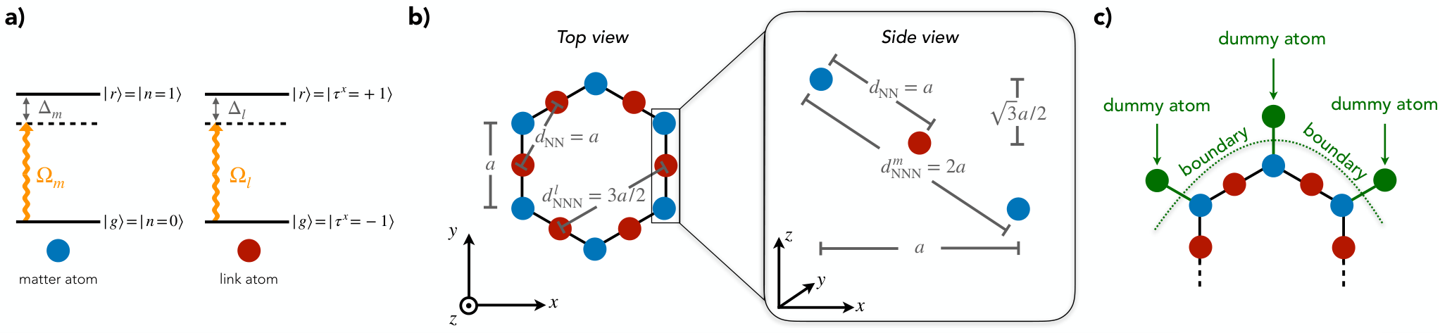
The scheme we propose in this Article is particularly suitable for Rydberg atom arrays because we require 1) control over the real-space configuration of atoms, 2) strong nearest-neighbor density-density interactions and 3) driving a two-level system. The microscopic Hamiltonian has been introduced in the main text in Eq. (3) and contains only nearest-neighbor interactions as well as an on-site drive, which is detuned from the ground state to Rydberg transition by and , see Fig. S11a. The detuning has two contributions : on the one hand side the term is essential for the LPG protection and appears when rewriting the Pauli spins as . On the other hand, the term enables to arbitrarily tune the electric field and chemical potential in Hamiltonian (4).
The LPG term requires the Rydberg-Rydberg interaction between matter and link atoms at each vertex to have the same strength , see Fig. 1a. The interaction strength between two atoms both excited to a Rydberg state scales as for large distances, where is a constant containing details of the internal atomic structure and is the distance between the two atoms. Therefore, to have equal interaction strength between link and matter atoms, we require a tetrahedron geometry at each vertex as shown in Fig. 1a and S11b. We define as the length of the edge of the honeycomb lattice. Link atoms are located on the center of edges and neighboring link atoms have a distance of and thus we require the plane of matter and link atoms to have a distance of . Since the honeycomb lattice is bipartite, we suggest to lift matter atoms in sublattice A (B) up (down) to decrease next-nearest neighbor interactions between matter atoms. These undesired next-nearest neighbor interactions can be estimated, see Fig. S11b, and we find that the nearest neighbor matter-matter interaction has strength and the next-nearest neighbor link-link interaction has strength .
Note that in an experimental setup the system has boundaries and here we want to discuss the LPG term at the boundary, see Fig. S11c. In particular, we want to consider the case where the boundary cuts through links of the honeycomb lattice, i.e. the boundary vertices have missing link atoms. To this end, we introduce dummy atoms in Fig. S11c which are not real atoms but instead substitute the missing link atom in the LPG term Eq. (2) by setting the corresponding dummy link to a constant value . This yields additional detuning terms for all atoms on the boundary vertices. For technical purposes, instead of individually addressing the detuning on only boundary sites one could introduce real auxiliary atoms on the boundary, which are excited to a Rydberg state different from the matter and link atoms. This allows to shift the Rydberg state of the matter and link atoms on the boundary, i.e. adding the required detuning, while the auxiliary atom is not affected by the driving field .
VI Disorder-free localization
Disorder-free localization (DFL) is a phenomenon that has been studied in theories with local symmetries Smith et al. 2017; Smith et al. 2018; Karpov et al. 2021; Halimeh et al. 2021b; Halimeh et al. 2022b; Chakraborty et al. 2022. Here, we use the microscopic model (3) – as it would be implemented in an experimental setup – and show DFL behaviour in a small-scale exact diagonalization (ED) simulation for the case of matter. In particular, the observation of DFL would be an accessible experimental probe since it only requires to prepare the system in two different initial product states and time-evolve them under the microscopic Hamiltonian.
The key idea is the following: Consider a system with two subsytems A and B and an initial state, where all matter sites in subsystem A (B) are occupied (empty). We let the state time-evolve under a invariant Hamiltonian and ask whether the matter excitations stay localized in subsystem A or delocalize equally across subsystem A and B. Hence, the quantity of interest is the time-averaged imbalance of matter excitations at time between the subsytems given by
| (S37) |
where is the expectation value of total matter excitations in subsystem A (B) at time and denotes the system size.
The eigenstate thermalization hypothesis (ETH) claims that eventually approaches its thermal equilibrium value. In DFL, this hypothesis is believed to be broken for gauge-noninvariant initial states . In the following sections we want to examine this behaviour on the example of 1) the minimal “Mercedes star” lattice with coordination number [] as presented in the main text and 2) on a Zig-Zag chain [], which would be experimentally easier to reach large system sizes. In both examples, we performed ED studies of the microscopic Hamiltonian (3) in small, numerically accessible systems.
VI.1 Mercedes star

Let us first consider the gauge-invariant initial state with and matter excitations being distributed as described above. The Mercedes star model with four matter sites and six links is illustrated in the inset of Fig. 3a. For this initial state, we can compute the imbalance from the thermal ensemble as predicted by ETH (see also Ref. Halimeh et al. 2021b; Halimeh et al. 2022b, SI B) and find that indeed the system fully delocalizes . Comparing this to the ED results in Fig. 3a, we find that the time-average imbalance quickly vanishes as expected.
The situation changes for the gauge-noninvariant initial state . For this state the matter excitations should be located again only in subsystem A but the links should be in eigenstates as indicated in Fig. 3a. Therefore, is an equal superposition of all possible gauge sectors . While still , as we have verified numerically, we find that the state does not thermalize under time-evolution with as shown in Fig. 3a.
For dynamics under a perfectly gauge-invariant Hamiltonian, , the intuitive picture is the following: When the system is initialized in a superposition of all gauge sectors, the system independently time evolves in each of these (uncoupled) gauge sectors. In each gauge sector the system has different background charges, which affects the spreading of the matter excitations, and ultimately the average is taken over all these gauge sectors. This effectively induces disorder in the system, which can lead to localization Smith et al. 2017.
While this interpretation holds for gauge-invariant Hamiltonians, we want to note the differences to our scheme here. Firstly, we generate the local symmetries in our system through local pseudogenerators , which yield an even enriched symmetry structure because the system has three emerging local symmetry sectors as shown in Fig. 1c. This has been discussed previously Halimeh et al. 2022b for D systems. Secondly, the microscopic Hamiltonian explicitly breaks the local symmetry generated by the LPG terms, , to induce dynamics in the system (note that the gauge symmetry is only approximate and not exact). Hence, the weak drive has to be considered as an error term, which eventually leads to thermalization of the system for long times. However, at experimentally relevant timescales we find a clear pre-thermal plateau indicating DFL as shown in Fig. S12a. The parameters used in the ED calculation are shown in the inset of Fig. S12a.
VI.2 Zig-Zag chain
The Mercedes star model is a numerical toy model with coordination number . A truly D model with can be realized on the honeycomb lattice but requires a large number of qubits/atoms. Therefore, as a first step to probe the proposed model, we suggest to implement a Zig-Zag chain with periodic boundary conditions, where each site of the chain is connected to a dummy atom, see Fig. S12b and SI V. This additional dummy atom ensures coordination number such that the LPG protection scheme becomes fully applicable.
In Fig. S12b, we show results of an ED study in a Zig-Zag chain with four matter sites and four links with periodic boundary conditions. Again, we can define a subsystem A (B), where matter excitations are located at time . Furthermore, the gauge-invariant state and gauge-noninvariant state differ by the configuration of the link atom. For both initial states, we expect the thermal expectation value of the imbalance, Eq. (S37), to vanish
Again, we find a clearly different behavior after time-evolving under the microscopic Hamiltonian and evaluating the time-averaged imbalance. However, the observed dynamics is slower than in the Mercedes star model. The parameters used in the ED calculation are shown in the inset of Fig. S12b.
VII Schwinger effect

The Schwinger effect is a non-perturbative effect from quantum electrodynamics that describes the production of matter excitations from vacuum Schwinger 1951. Due to the weak coupling constant of quantum electrodynamics this effect is only expected to appear at very strong electric fields and has not been observed. LGTs were originally introduced to study the effects of strong coupling in gauge theories Wilson 1974 and are therefore a candidate theory to also study the physics of the Schwinger effect. Recently, digital quantum simulation of the D Schwinger model on the lattice have examined the Schwinger effect Martinez et al. 2016. Here, we want to present an experimentally measurable quantity by considering the pairwise production of matter excitations. While the potential between two static charges is of theoretical interest and used as a signature of the Schwinger effect Sala et al. 2018, it is numerically challenging to extract in D and is a topic for future studies.
Our effective model (4) allows to explore the Schwinger effect in a mLGT in D, which has not yet been observed. The experimental protocol starts by initializing a gauge-invariant state without any matter excitations in one of two vacua, i.e. either all links in or , which is a simply product state. Then, the system is quenched with the microscopic Hamiltonian (3) for time yielding . The effective model (4) with quantum- matter, which we expect to correctly capture the physics, contains pairing terms yielding pair creation processes from vacuum. As soon as the matter excitations are created, they move apart due to the hopping term and interact with the gauge field, which makes the prediction of the dynamics very challenging.
Therefore, an easily accessible quantity to probe the Schwinger effect is the gauge-invariant production rate of matter excitations. To this end, we let the system time-evolve and calculate
| (S38) |
which projects onto the gauge sector and gives the expectation value of the total number of matter excitations in the system.
We calculate for for different electric fields and chemical potentials , see Eq. (3), for . In Fig. S13a we plot the timetraces for some set of parameters and we have checked that the maximal time-evolution time of captures the peak of each timetrace.
Each timetrace has different amplitude and timescale and therefore only considering at a fixed time is not sufficient to extract the productivity of creating matter excitations from vacuum. To this end, we take the maximum value of each timetrace for each , which is plotted in Fig. 3b in the main text.
We find that for some the production of matter excitations is significantly higher than for others. An intuitive picture is that a pair of matter excitations costs an energy (mass of matter excitations) and due to Gauss’s law, the two matter excitations have to be connected by an electric string, which costs . Therefore, if the process is on resonance we expect a high production rate of matter pairs. Note that have to be determined from Tab. SII and are not simply given by .
Besides the resonances described above, there are several more processes that would have to be taken into account. E.g. two neighboring matter excitations repel each other with strength ; Eq. (II.3); matter excitations are mobile; plaquette interaction compete with the electric field; finite size effects etc. Due to these competing interactions, it is very hard to gain a complete picture and thus large-scale numerical simulations as well as experimental observations are needed. Nevertheless, small-scale numerical calculations of the microscopic model show promising signatures of the Schwinger effect.
An additional feature we monitored in our ED study is the role of gauge-noninvariant dynamics. In Eq. (S38) we project out unphysical states. In contrast we can do the same analysis as before but without projecting on the target gauge sector, which is shown in Fig. S13b. We find regions with additional resonances, which are caused by gauge-symmetry breaking processes. However, the resonances we find with projecting on the gauge sectors are not altered, which is an evidence that the physics is purely determined by -invariant dynamics.
VIII DMRG in the ladder
In Fig. 2 in the main text, we map out limiting cases of the ground-state phase of the effective model (4). A numerically more accessible and experimentally realizable model is the mLGT coupled to matter on a ladder. While the ladder geometry is not D but mixed-D, it has coordination number and therefore is applicable for our proposed LPG term (2). Thus, the effective Hamiltonian only has to be modified for the plaquette interaction because the plaquettes on a ladder have four instead six edges; note that we anticipate the plaquette terms to be even stronger in the ladder and we choose as found in SI II.2 in Eq. (S16).
For our numerical simulations, we use Hamiltonian (4) with , i.e. we have a global symmetry for the matter, and we tune the electric field and chemical potential for fixed tunneling and plaquette interactions and . Using the density matrix renormalization group (DMRG) technique, we calculate the ground state of the above described Hamiltonian on a ladder with plaquettes.
From the ground state calculated in DMRG, we obtain the average matter excitation density – an experimentally directly accessible quantity, e.g. by taking snapshots in the atomic ground state and Rydberg basis (see Fig. 1a). As shown in Fig. 3c, the system is in a matter vacuum for large similar to the D case. For decreasing , we find a sharp increase of matter excitations indicating a phase transition as shown in Fig. S14a. At the same critical electric field value, the plaquette term shows a sharp feature; note that and thus the plaquette expectation value is negative indicated by the reversed sign on the plot label in Fig. S14b.
Moreover, we show a similar scan of parameters but now we fix the electric field while scanning the chemical potential . We find consistent behaviour with Fig. 2a, i.e. a sharp transition into the vacuum phase, see Fig. S14c and d.
To characterize the different phases and its phase transitions requires more elaborate studies of our effective model on the ladder and is a topic for future studies. We emphasize that due to its numerical accessibility and experimental feasibility, the ladder model is a promising playground to probe lattice gauge theories coupled to dynamical matter beyond D.
In the following, we discuss numerical details of the DMRG calculation. We use the TeNPy package Hauschild et al. 2018; Hauschild and Pollmann 2018 to find the ground state of Hamiltonian (4) with . Note that while this Hamiltonian conserves the particle number, we do not run the DMRG simulation in a fixed particle number sector. For a given set of Hamiltonian parameters, we find the global ground state, and can therefore use the average matter density as an observable. In the DMRG simulation, we enforce the system to be in the target gauge sector by adding a large energy penalty term proportional to Gauss’s law (1) to the Hamiltonian. The ground state will therefore always fulfill Gauss’s law by construction. We carefully checked our numerical results for convergence, see Fig. S14.
IX Thermal deconfinement
In the main text and Methods section, we discuss a thermal deconfinement phase transition in a classical limit of the Hamiltonian (4), see Fig. 3d. Here we provide numerical details about our Monte Carlo simulations as well as supplementary results. The Monte Carlo simulations are implemented in C++ using the Boost C++ libraries. The lattice is represented as a graph which simplifies many operations involving nearest and next-nearest neighbors in a honeycomb lattice. For I/O operations, multiprocessing and postprocessing, we use Python (NumPy, SciPy, Python multiprocessing, Matplotlib).
We derive the classical model from the effective Hamiltonian (S13) with matter in the gauge sector , see Fig. S15d. To obtain a purely classical Hamiltonian (energy functional), we remove the matter and gauge field dynamics by setting , which yields (neglecting constant terms)
| (S39) | ||||
The energy is fully determined by the configuration of matter excitations and electric fields . The model should still be understood as an effective theory derived from the microscopic model Eq. (3). Hence, the drive and detunings determine the coupling strength of , , and , see Tab. SII. In our example, we have chosen the experimentally realistic parameters , and , which yields , , , . Note that the electric field term can be tuned independently by the link detuning .
To probe (de)confinement, we dope the system with exactly two matter excitations in all simulations (see Methods). The Monte Carlo simulations are based on Metropolis-Hastings sampling using move and plaquette updates presented in Fig. S15a.
At the beginning of each simulation, the system thermalizes for steps. Subsequently, we record samples with steps between each other. In Fig. S16, we show exemplary thermalization and autocorrelation plots for . We take the autocorrelation between snapshots into account for every error bar.
We simulate the system at for system size , , and on a honeycomb lattice with open boundaries. For each sample, we measure 1) the percolation strength, i.e. #(strings in the largest percolating string-cluster)/#(bonds), 2) the total number of strings, 3) the size of the largest string-cluster, and 4) the Euclidean distance between the two matter excitations. We illustrate two snapshots from the deconfined and confined regime in Fig. S15b.
In Fig. S17 we show Monte Carlo results for system size and . We observe a clear change of behaviour in all above discussed quantities, which signals a thermal deconfinement phase transition. For low temperatures, the percolation strength vanishes. At a critical temperature , the percolation strength abruptly increases, i.e. the string-net percolates and the matter excitations are deconfined. At the same critical temperature , the Euclidean distance between the two matter excitations drastically increases to roughly the system size. We note that finite-size effects strongly influence for small system sizes. However, the transition becomes generally sharper for larger lattice sizes as expected.