Extreme mass ratio inspirals into black holes surrounded by matter

Consider a Hamiltonian system of $N$ degrees of freedom with the Hamiltonian $H(q_{i},p_{i})$ satisfying the following conditions:

1. 1.

   The system possesses $N$ linearly independent isolating integrals of motion $I_{i},\kern 5.0pt\{I_{i},I_{j}\}=0,\kern 5.0pti,j=1,\ldots N$

2. 2.

   Motion in the phase space is bounded.

According to the Liouville-Arnold theorem (see for example (Wiggins; arnold2007mathematical)), the motion is then confined to an $N$-dimensional subset of the phase space diffeomorphic to the torus $\mathbb{T}^{N}$. The particular torus on which the selected trajectory lies is defined by $N$ parameters $J_{i}$ called actions and can be parametrized by $N$ periodic angles $\psi_{i}\in(0,2\pi)$. Angles are canonically conjugate to actions and together they are known as action-angle coordinates.

If we perform a canonical transformation to action-angle coordinates we find that the new form of the Hamiltonian has one remarkable property, it depends only on the actions

$\displaystyle(q_{i},p_{i})\rightarrow(\psi_{i},J_{i}),\kern 5.0ptH(q_{i},p_{i})\rightarrow H(J_{i})\,.$

Consequently the solution to Hamilton equations is trivial

$\displaystyle\begin{aligned} J_{i}(t)=\mathrm{constant},\\ \psi_{i}(t)=\Omega_{i}t+\psi_{0i},\end{aligned}$

(1)

where $\Omega_{i}=\frac{\partial H(J_{j})}{\partial J_{i}}$ are the frequencies of motion. Inserting the solution (1) into the transformation relations we obtain

$\displaystyle q_{i}=q_{i}(\psi_{j}(t),J_{j}),\kern 5.0ptp_{i}=p_{i}(\psi_{j}(t),J_{j})\,.$

(2)

Thus, finding the transformation from action-angle coordinates to the original coordinates is equivalent to solving the Hamilton equations of motion in the original coordinates $(q_{i},p_{i})$.

In the particular case of a separable system, in which the motion is periodic in coordinate $q_{i}$, the corresponding action can be computed using the formula (Lichtenberg)

$\displaystyle J_{i}=\frac{1}{2\pi}\oint p_{i}\mathrm{d}q_{i}\,,$

(3)

where the integral is taken along a complete time period of the motion.

Unfortunately, there are very few examples in which the integral (3) can be evaluated in a closed form. One such example is the harmonic oscillator whose Hamiltonian can be transformed as

$\displaystyle H(q,p)=\frac{p^{2}}{2m}+\frac{1}{2}m\Omega^{2}q^{2}\rightarrow\kern 5.0ptH(\psi,J)=\Omega J\,,$

(4)

while the transformation relations are given by

$\displaystyle q=\sqrt{{\frac{2J}{m\Omega}}}\sin\left(\psi\right),\hskip 35.0ptp=\sqrt{2J\Omega\,m}\cos\left(\psi\right).$

(5)

In these relations one can clearly see the familiar solution to the harmonic oscillator problem.

At this point one can surely ask whether it is possible to perform such a transformation in case of a more complicated integrable system or even in a case of a slightly perturbed integrable system. This question leads us directly to the Lie series formalism.

The Lie series are a class of canonical transformations defined by an arbitrary generating function $\omega(q_{i},p_{i})$ (details in Refs (Efthymiopoulos11; cary1981lie; Deprit)). We will first describe this on the best known case of time evolution. Denoting $z_{i}$ as the phase space coordinates, the evolution equation can be written as

$\displaystyle\frac{\mathrm{d}z_{i}}{\mathrm{d}t}=\{z_{i},H\}.$

(6)

The solution to this equation can then be found using the Taylor expansion where the time derivative is replaced by the Poisson bracket with the Hamiltonian, which is a consequence of eq. (6). Denoting $z_{i}(0)=z_{i}$ we have

$\displaystyle\begin{split}z_{i}(t)=z_{i}+\{z_{i},H\}t+\frac{1}{2}\{\{z_{i},H\},H\}t^{2}+\ldots=\\ =\exp(t\pounds_{H})z_{i}\,,\end{split}$

(7)

where the operator $\pounds_{g}$ is defined as $\pounds_{g}f=\{f,g\}$. The operator $\pounds_{g}$ is called Lie derivative because in the geometrical formulation of Hamiltonian mechanics we have $\pounds_{g}=\pounds_{X_{g}}$ where $X_{g}$ is the Hamiltonian vector field associated with the function $g$.

If we now make an exchange: $H\leftrightarrow\omega(q_{i},p_{i}),\kern 5.0ptt\leftrightarrow\varepsilon$ where $\varepsilon$ is a small parameter, we can define a new transformation

$\displaystyle Z_{i}=z_{i}(\varepsilon)=\exp(\varepsilon\pounds_{\omega})z_{i}\,.$

(8)

This transformation is indeed canonical as the Poisson brackets are preserved due to the following identity (Deprit):

$\displaystyle\{\exp(\pounds_{\omega})f,\exp(\pounds_{\omega})g\}=\exp(\pounds_{\omega})\{f,g\},$

(9)

which leads to $\{z_{i},z_{j}\}=\{Z_{i},Z_{j}\}$. Another useful identity is the inverse relation for the Lie operator

$\displaystyle\big(\exp(\varepsilon\pounds_{\omega})\big)^{-1}=\exp(-\varepsilon\pounds_{\omega}).$

(10)

Having introduced the Lie series formalism, we can now use it to approximately transform a Hamiltonian into action-angle coordinates, or to be more specific, to find the so called Birkhoff normal form of a Hamiltonian.

Assume we have a Hamiltonian in the form:

$\displaystyle H^{(0)}=H_{0}(J_{i})+\displaystyle\sum_{j=1}\varepsilon^{j}H_{j}^{(0)}(\psi_{i},J_{i})\,,$

(11)

where $H_{0}(J_{i})$ is a well known integrable Hamiltonian already expressed in the action-angle form while the other part is expanded in a small perturbation parameter $\varepsilon$. Computing the Birkhoff normal form of $H^{(0)}$ actually means eliminating the angle variables from the Hamiltonian.

Starting from the first order of the perturbation we decompose the Hamiltonian $H_{1}^{(0)}$ into the part which does not depend on the angles and the other which does: $H_{1}^{(0)}=Z_{1}(J_{i})+h_{1}(\psi_{i},J_{i})$. If we then act with the Lie operator on $H^{(0)}$ we get

$\displaystyle\exp(\varepsilon\pounds_{\omega_{1}})H^{(0)}=H_{0}+\varepsilon Z_{1}+\varepsilon\{H_{0},\omega_{1}\}+\varepsilon h_{1}+\mathcal{O}(\varepsilon^{2}).$

(12)

Since $h_{1}$ is to be eliminated, the terms proportional to $\varepsilon$ have to satisfy:

$\displaystyle\kern 5.0pt\{H_{0},\omega_{1}\}+h_{1}\stackrel{{\scriptstyle!}}{{=}}0.$

(13)

This is called homological equation which has to be solved for the so far unknown generating function $\omega_{1}$. Once we have found $\omega_{1}$ we can compute a new form of our Hamiltonian

$\displaystyle H^{(1)}=\exp(\varepsilon\pounds_{\omega_{1}})H^{(0)}=H_{0}(J_{i})+\varepsilon Z_{1}(J_{i})+\mathcal{O}(\varepsilon^{2}).$

(14)

Thus, we have our Hamiltonian in the action-angle variables up to the first order in $\varepsilon$. We can now proceed in a similar fashion, i.e., solving another homological equations and so on until arriving at a desired order $n$ in which the Hamiltonian reads

$\displaystyle\begin{split}H^{(n)}=\exp(\varepsilon^{n}\pounds_{\omega_{n}})\exp(\varepsilon^{n-1}\pounds_{\omega_{n-1}})\ldots\exp(\varepsilon\pounds_{\omega_{1}})H^{(0)}=\\ =U(\omega_{i})H^{(0)},\end{split}$

(15)

where the notation $U(\omega_{i})$ is used just for brevity to represent the $n$ canonical transformations applied. Furthermore, $H^{(n)}$ can be decomposed into

$\displaystyle\begin{gathered}H^{(n)}=H_{NF}(J_{i})+R^{(n)}(\psi_{i},J_{i})\,,\\ H_{NF}(J_{i})=H_{0}(J_{i})+\displaystyle\sum_{j=1}^{r}\varepsilon^{j}Z_{j}(J_{i});\kern 5.0ptR^{(n)}(\psi_{i},J_{i})=\mathcal{O}(\varepsilon^{n+1}),\end{gathered}$

where $H_{NF}$ is the Birkhoff normal form of $n$th order, while $R^{(n)}$ is a remainder which can be neglected as $\varepsilon^{n+1}$ is a sufficiently small number. The Birkhoff normal form now allows us to compute the frequencies of motion which tell us how the new angles evolve (see Eq. (1)). The old coordinates can now be expressed in terms of the new ones

$\displaystyle\psi^{(0)}=U(\omega_{i})\psi,\kern 5.0ptJ^{(0)}=U(\omega_{i})J\,.$

(18)

Inserting Eq. (1) into the transformation relation (2) gives us an approximative solution to the equation of motion with the error given by the size of the remainder $R^{(n)}$.

The Lie series is generally only asymptotic; there may exist a maximum order above which the approximation becomes less and less precise. The question of convergence of canonical perturbation theory is tied to the existence of small divisors and resonances, and the Lie series is not guaranteed to converge everywhere even in fully integrable systems (see, e.g., Refs (Efthymiopoulos11; arnold2007mathematical)). We shall demonstrate the issues with resonances also in Sec. III.4.

Picture a black hole of mass $M$ encircled by a rotating gravitating ring with mass $\mathcal{M}_{\rm r}$ and radius $r_{\rm r}\gg M$ much larger than the black hole horizon. What are going to be the leading-order effects of the ring on the gravitational field near the black hole? It was found already by Thirring in 1918 (thirring1918wirkung; Mashhoon:1984fj) that the local inertial system inside a light, thin rotating shell is rotating with respect to the inertial system at infinity with an angular velocity

$\displaystyle\Omega_{\rm Thir}=\frac{2\mathcal{J}_{\rm sh}}{r_{\rm sh}^{3}}\,,$

(19)

where $\mathcal{J}_{\rm sh},r_{\rm sh}$ are the total angular momentum and radius of the shell. Similarly, the rate of time inside the shell is redshifted with respect to observers at infinity by the gravitational potential on the surface of the shell

$\displaystyle z_{\rm sh}=\frac{\mathcal{M}_{\rm sh}}{r_{\rm sh}}\,,$

(20)

where $\mathcal{M}_{\rm sh}$ is the total mass of the shell.

Based on the works of Refs Will:1974zz; Cizek:2017wzr, we show in Appendix A that a similar effect occurs in the case of the ring-hole system. Specifically, the inertial frame near the center of a ring of angular momentum $\mathcal{J}_{\rm r}$ and Schwarzschild radius $r_{\rm r}$ rotates, to leading order in $r_{\rm r}\gg M\gg\mathcal{M_{\rm r}}$, with an angular velocity

$\displaystyle\Omega_{\rm in}=\frac{2\mathcal{J}_{\rm r}}{r_{\rm r}^{3}}+\mathcal{O}(r_{\rm r}^{-5})\,.$

(21)

We assume that the ring-like structure is moving approximately as a test body in the black-hole field, so to leading order we have $\mathcal{J}_{\rm r}=\mathcal{M}_{\rm r}\sqrt{Mr_{\rm r}^{2}/(r_{\rm r}-3M)}$ and we can write

$\displaystyle\Omega_{\rm in}=2\mathcal{M}_{\rm r}\sqrt{\frac{M}{r_{\rm r}^{5}}}\left(1+\frac{3M}{2r_{\rm r}}\right)+\mathcal{O}(r_{\rm r}^{-9/2})\,.$

(22)

Additionally, the internal frame is redshifted by a factor

$\displaystyle z_{\rm in}=\frac{\mathcal{M}_{\rm r}}{r_{\rm r}}\left(1+\frac{M}{r_{\rm r}}\right)+\mathcal{O}(r_{\rm r}^{-3})\,.$

(23)

Finally, the gravitational field near the black hole will also have a tidal contribution from the ring. Apart from assuming that the black hole is static in the “internal” inertial frame, we also truncate the tides to leading quadrupolar order. Then we obtain the metric valid near the black hole (see Appendix A for details):

	$\displaystyle\begin{split}&\mathrm{d}s^{2}_{r\ll r_{\rm r}}=-\left(1-\frac{2M}{r}\right)(1+2\nu_{Q})\mathrm{d}t^{2}+\frac{1+2\chi_{Q}-2\nu_{Q}}{1-2M/r}\mathrm{d}r^{2}\\ &\phantom{\mathrm{d}s^{2}=}+(1-2\nu_{Q})r^{2}\left[(1+2\chi_{Q})\mathrm{d}\vartheta^{2}+\sin^{2}\!\vartheta\mathrm{d}\varphi^{2}\right]\,,\end{split}$			(24)
		$\displaystyle\nu_{Q}\equiv\frac{Q}{4}\left[r(2M-r)\sin^{2}\!\vartheta+2(M-r)^{2}\cos^{2}\!\vartheta-6M^{2}\right]\,,$		(25)
		$\displaystyle\chi_{Q}\equiv QM(M-r)\sin^{2}\!\vartheta\,,$		(26)

where $Q\equiv\mathcal{M}_{\rm r}/r_{\rm r}^{3}$ is the quadrupole perturbation parameter and $t,r,\vartheta,\phi$ are Schwarzschild-like coordinates in the local frame. The local metric is approximately vacuum, static and axisymmetric with respect to the local time and azimuthal angle $t,\varphi$ with corresponding Killing vectors $\xi^{\mu}_{(t)}=\delta^{\mu}_{t},\,\xi^{\mu}_{(\varphi)}=\delta^{\mu}_{\varphi}$. As such, it is an approximate Weyl metric (weyl1917gravitationstheorie; Griffiths:2009dfa).

The form (24) of the metric is valid only for $r\ll r_{\rm r}$ and rings that are not compact, $\mathcal{M}_{\rm r}\ll r_{\rm r}$. Specifically, it neglects all terms starting from $\mathcal{O}(r_{\rm r}^{-4})$ and $\mathcal{O}(\mathcal{M}_{\rm r}^{2})$. Also, as already discussed, the local coordinates are related to the coordinate time and azimuthal angle $T,\phi$ of static observers at infinity as

		$\displaystyle\mathrm{d}T=(1+z_{\rm in})\mathrm{d}t\,,$		(27)
		$\displaystyle\mathrm{d}\phi=\mathrm{d}\varphi+\Omega_{\rm in}\mathrm{d}t\,.$		(28)

This has to be taken into account when predicting observations from the dynamics in the metric field (24).

Note that this framework is very flexible, since it does not necessarily fix the relationship between $z_{\rm in},\Omega_{\rm in}$ and $Q$. For more general matter distributions than a thin ring, these parameters can be computed separately and fed into the formalism the same way as it is done here. However, one case which we do not treat are time-dependent and non-axisymmetric perturbations which would correspond to perturbers orbiting our EMR binary at intermediate distances. The possibility of inclusion of this case is discussed in Sec. VI.

We would now like to apply the aforementioned theory to the Hamiltonian

$\displaystyle H_{\rm tot}=\frac{1}{2}g^{\mu\nu}p_{\mu}p_{\nu}\,,$

(29)

where $g^{\mu\nu}$ is our background metric (24) and the four-momentum $p_{\mu}$ is normalized to unity, i.e. $g^{\mu\nu}p_{\mu}p_{\nu}=-1$. We will first start with the well known Schwarzschild Hamiltonian ($Q=0$)

$\displaystyle H_{\rm Schw}=\frac{1}{2}\left[\frac{-1}{1-\frac{2M}{r}}p_{t}^{2}+\bigg(1-\frac{2M}{r}\bigg)p_{r}^{2}+\frac{1}{r^{2}}\left(p_{\theta}^{2}+\frac{p_{\phi}^{2}}{\sin^{2}\theta}\right)\right].$

(30)

Unfortunately this Hamiltonian cannot be put exactly into the action-angle variables like the Kepler Hamiltonian. Nevertheless $H_{\rm Schw}$ remains separable which means that by adopting a new evolution parameter $\lambda$ defined as $\mathrm{d}\tau=r^{2}\mathrm{d}\lambda$ we can separate our Hamiltonian to a radial and an angular part. The parameter $\lambda$ is a special case of the Carter-Mino time Carter:1968rr; Mino used for similar reasons in the Kerr spacetime. The Hamiltonian generating evolution in $\lambda$ (see Appendix B) can be written as

$\displaystyle H_{{\rm Schw}(\lambda)}=\frac{1}{2}r^{2}(g_{S}^{\mu\nu}p_{\mu}p_{\nu}+1)=H_{\rm rad}+H_{\rm ang}\,,$

(31)

where

$\displaystyle H_{\rm rad}$

$\displaystyle=\frac{1}{2}r^{2}\left[-\frac{1}{1-\frac{2M}{r}}p_{t}^{2}+\bigg(1-\frac{2M}{r}\bigg)p_{r}^{2}+1\right]\,,$

(32)

is the radial part and

$$H_{\rm ang}=\frac{1}{2}\left(p_{\theta}^{2}+\frac{p_{\phi}^{2}}{\sin^{2}\theta}\right)$$

is the angular part of the Hamiltonian.

Having separated our Hamiltonian we can now perform the transformation of the respective parts into action-angle coordinates. Since the metric does not depend on $\phi$, the specific angular momentum $p_{\phi}=J_{\phi}=L_{z}$, i.e. the $z$-component of the angular momentum per unit mass, is already an action variable while for the $\theta$ part we have

$$J_{\theta}=\frac{1}{2\pi}\oint p_{\theta}\mathrm{d}\theta=L-J_{\phi}$$

(33)

where $L$ is the specific total angular momentum. The action $J_{\theta}$, thus, describes the part of angular momentum associated with non-equatorial motion.¹¹ 1 For equatorial motion $J_{\theta}=0$. The angular part of the Hamiltonian in the action-angle coordinates reads

$$H_{\rm ang}=\frac{1}{2}(J_{\theta}+J_{\phi})^{2}\,.$$

(34)

The conjugate angles $\psi_{\theta}$ and $\psi_{\phi}$ to the actions $J_{\theta}$ and $J_{\phi}$ are obtained by canonical transformations, which can be found in Appendix B.

Let us now discuss the more difficult part, which involves the radial part $H_{\rm rad}$. In Eq. (32) we replace the $p_{t}$ component of the four-momentum by the specific energy of the system $E=-p_{t}$ and we perform an expansion of the system around a stable circular orbit ($r=r_{c},p_{r}=0,E=E_{c}$). The perturbation parameter along which the expansion takes place is the distance from the circular orbit (something akin to the eccentricity). We assume that the relevant phase space coordinates deviate from those corresponding to the circular orbit like

$\displaystyle r-r_{\mathrm{c}}=\mathcal{O}(\varepsilon)=p_{r},\kern 5.0ptE-E_{c}=\delta E=\mathcal{O}(\varepsilon^{2})\,,$

(35)

where $\varepsilon$ is a book-keeping parameter telling us how big each term in our expansion is. Keep in mind that $\varepsilon$ is not the perturbation parameter, after the computation we can just set it to $\varepsilon=1$.

As the radius $r_{\mathrm{c}}$ is the minimum of the effective potential $V_{\rm eff}=H_{\rm rad}$ (see, e.g., (Chandrasekhar:1985kt)), the first post-circular approximation is the harmonic oscillator. After performing a transformation similar to Eq. (4) (details in Appendix B) we get the radial part in the form

$\displaystyle H_{\rm rad}$

$\displaystyle=K_{0}+K_{2}\delta E+J_{r}\Omega_{rc}+R(\delta E,\psi_{r},J_{r})\,,$

where $K_{0}$ and $K_{2}$ are constants and $\Omega_{rc}$ is the frequency of the respective harmonic oscillator (Appendix B).

Neglecting the remainder $R(\delta E,\psi_{r},J_{r})=\mathcal{O}(\varepsilon^{3})$ we could accurately describe quasi-circular orbits. However we would like to describe nearly all the bound orbits with sufficient precision, which is why we implement the canonical perturbation theory as discussed in the next section.

In this section we finish the construction of the approximative Hamiltonian system of a Schwarzschild with a ring in action-angle variables. First, we perform two normalization steps, as described in Sec. II.2. This implies finding two generating functions $\omega_{1}$ and $\omega_{2}$ to be used in the Lie operators acting on the Hamiltonian $H_{{\rm Schw}(\lambda)}$

$$\exp(\pounds_{\omega_{2}})\exp(\pounds_{\omega_{1}})H_{{\rm Schw}(\lambda)}=H_{\rm NS}(J_{r},J_{\theta})+\mathcal{O}(\varepsilon^{5})\,.$$

(36)

For the purposes of our study we deem approximation (36) to be sufficiently describing geodesic bound orbits around a Schwarzschild black hole, hence, we can now add the ring-like source.

Our initial Hamiltonian (29) can be naturally split into the Schwarzschild and the ring part as in the case of the linearly perturbed metric (24)

$$H_{\rm tot}=H_{{\rm Schw}(\lambda)}+QH_{\rm ring}\,.$$

(37)

The perturbation part is then transformed into the same coordinates as the Schwarzschild part

$$\exp(\pounds_{\omega_{2}})\exp(\pounds_{\omega_{1}})H_{\rm ring}=H_{Q1}+\mathcal{O}(\varepsilon^{5})\,,$$

(38)

while the terms of higher order in $\varepsilon$ are neglected. And, thus, the total Hamiltonian reads:

$$H_{\rm tot}=H_{\rm NS}(J_{r},J_{\theta})+QH_{Q1}(\psi_{r},\psi_{\theta},J_{r},J_{\theta})+\mathcal{O}(\varepsilon^{5})\,.$$

(39)

The last step in our computation is to solve the homological equation for the function $\chi$ in order to eliminate the angles from $H_{Q1}$.²² 2 Note that now $Q$ is the perturbation parameter. After this, the total Hamiltonian reads

	$\displaystyle H_{\rm tot}$	$\displaystyle=H_{\rm NS}(J_{r},J_{\theta})+QZ_{Q1}(J_{r},J_{\theta})+\mathcal{O}(Q^{2})$
		$\displaystyle=H_{\rm N}(J_{r},J_{\theta})+\mathcal{O}(Q^{2})\,.$		(40)

The original coordinates can be expressed using the Lie operators as functions of the new ones as follows:

	$\displaystyle r$	$\displaystyle=\exp(Q\pounds_{\chi})\exp(\pounds_{\omega_{2}})\exp(\pounds_{\omega_{1}})r_{0}=U(\omega_{1},\omega_{2},\chi)r_{0},$
	$\displaystyle p_{r}$	$\displaystyle=U(\omega_{1},\omega_{2},\chi)p_{r_{0}},$		(41)
	$\displaystyle\theta$	$\displaystyle=\exp(Q\pounds_{\chi})\theta_{0},\;p_{\theta}=\exp(Q\pounds_{\chi})p_{\theta_{0}},\;\phi=\exp(Q\pounds_{\chi})\phi_{0}$

where $r_{0},p_{r_{0}},\theta_{0},p_{\theta_{0}}$ and $\phi_{0}$ are the original transformation functions given by Eqs. (B), (90), and (B) respectively in the Appendix B.

Solving the homological equation (13) at each step is quite straightforward, the relatively difficult part is finding the generating function $\chi$ as it involves two degrees of freedom. By expanding the Hamiltonians in parameters $\varepsilon$ and $Q$, the $h_{1}$ part of $H_{Q1}$, which is to be eliminated, takes form

$$h_{1}=\displaystyle\sum_{k,l}a_{kl}e^{i(k\psi_{r}+l\psi_{\theta})},$$

(42)

where the coefficients $a_{kl}$ are in fact functions of actions. The solution to Eq. (13) can then be expressed as:

$$\chi=\displaystyle\sum_{k,l}a_{kl}\frac{1}{i(k\Omega_{r0}+l\Omega_{\theta 0})}e^{i(k\psi_{r}+l\psi_{\theta})}$$

(43)

where $\Omega_{r0}=\frac{\partial H_{\rm NS}}{\partial J_{r}}$ and $\Omega_{\theta 0}=\frac{\partial H_{\rm NS}}{\partial J_{\theta}}$ are the frequencies of the Schwarzschild Hamiltonian obtained in (36). When close to resonances the denominator of this expression tends to zero which causes the remainder to be large, thus making the approximation less accurate as we shall see in the following section.

All the above-mentioned calculations involving canonical perturbation theory are included in the first part of our Supplemental material SupMat1.

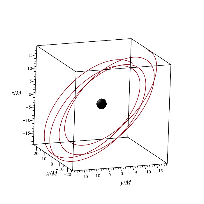
The analytical formulas (III.3) can be plotted for fixed values of the actions to illustrate our result (Fig. 1). It is clear from the figure that nonequatorial motion is no longer planar since the ring (located in the $z=0$ plane) breaks the spherical symmetry of the Schwarzschild spacetime.

Knowing the explicit expressions (III.3) and the approximate normal form of our Hamiltonian $H_{\rm N}(J_{i})$ (III.3) we have essentialy perturbatively solved the original equations of motion given by $H_{\rm tot}$. First we fix three of our new set of conserved actions and then compute the fourth so that the normalization condition

$\displaystyle H_{N}(J_{r},J_{\theta},\delta E,J_{\phi})=0$

(44)

is satisfied. Then, we find the frequencies of motion for our new angles as well as the relation between the coordinate time $t$ and $\lambda$

$\displaystyle\frac{\mathrm{d}\psi_{i}}{\mathrm{d}\lambda}=\frac{\partial H_{N}}{\partial J_{i}}=\Omega_{i}(J_{r},J_{\theta},\delta E,J_{\phi}),\hskip 25.0pt\frac{\mathrm{d}t}{\mathrm{d}\lambda}=\frac{\partial H_{N}}{\partial\delta E}.$

(45)

Finally we substitute the angles and actions into Eq. (III.3) to get the coordinates and their respective momenta as explicit functions of Mino time $\lambda$ $(x^{i}(\lambda),p_{i}(\lambda))$.

The evolution of the deviations from the exact solutions is governed by the remainder $R(\psi_{i},J_{i})$ which contains all the terms of the order $\mathcal{O}(\varepsilon^{5})$ and $\mathcal{O}(Q^{2})$. It is clear that the validity of our approximation not only depends on the fixed parameter $Q$ describing the gravitational field of our ring-like source, but also on all our actions $J_{r},J_{\theta},J_{\phi}$. The most straightforward way to test our approximation would be plotting and comparing our analytical solution to the numerical one. This is certainly illustrating, nevertheless, it is still useful to have some quantity to describe the deviation from the exact solution. For this purpose we can use quantities denoted as $\delta J_{i}$ which measures the relative error of the conservations of actions. The errors $\delta J_{i}$ can then be expressed as functions of actions $J_{i}$ in order to study the validity of the approximation (details are given in Appendix C).

In general, it can be said that the larger the value of $J_{r}$ is the less accurate the approximation becomes. Apart from that the approximation depends on the perturbation parameter $Q$ and the total angular momentum $L$. These two, however, are not independent from each other as increasing the value of $L$ is equivalent to increasing $Q$. This comes from the fact that $\nu_{Q}$ is not bounded by a fixed value of $Q$ instead we have $\nu_{Q}\sim r^{2}$ (see Eq. (25)) and $r\sim L^{2}$. We can, thus, conclude that it is the value of the quantity $QL^{4}/M^{2}$ that characterizes the entire strength of the perturbation.

The most general type of motion is the nonequatorial one, for which we have $J_{\theta}\neq 0$. The dependence of $\delta J_{r}$ and $\delta J_{\theta}$ on actions is the same as in the equatorial motion, what is new here, however, is the presence of the resonances of the form

$\displaystyle k\Omega_{r0}+l\Omega_{\theta 0}=0,\kern 5.0ptk,l\in\mathbb{Z}\setminus\{0\}\,,$

(46)

where $\Omega_{r0}$ and $\Omega_{\theta 0}$ are the Schwarzschild frequencies. When the orbit is close to these resonances the approximation is no longer reliable because the denominators in the expression (43) tend to zero. These small divisors then prevent the convergence of the normalization procedure (see, e.g., Efthymiopoulos11). In our particular case we only applied one generating function involving two degrees of freedom which is $\chi$ (used in Eq. (III.3)). From the analysis of the function $\chi$ and the Schwarzschild frequencies it becomes clear that the only ratios $\frac{\Omega_{r0}}{\Omega_{\theta 0}}$ present in the expansion (43) of $\chi$ are the $\frac{1}{2}$, $\frac{2}{3}$ and $1$. This is illustrated in Fig. 2, which depicts the resonance sets in the $J_{r}$-$J_{\theta}$ plane for a fixed value of $J_{\phi}$. It is important to stress at this point that even though $\Omega_{r0}$ depends explicitly on the total angular momentum $L=J_{\theta}+J_{\phi}$ it is correct to treat both angular actions separately. The same can be said for the dependence on $Q$, which is much more significant than that on $L$, e.g. smaller value of $Q$ shifts the resonance curves to larger values of $L$. This dependence can be understood from the substitution of the energy from constraint (44) in $\Omega_{r0}$, for which we have $E=E(Q,J_{r},J_{\theta},J_{\phi})\neq E(Q,J_{r},J_{\theta}+J_{\phi})$. Namely, in total the expression for the radial frequency reads $\Omega_{r0}=\Omega_{r0}(E(Q,J_{r},J_{\theta},J_{\phi}),J_{r},J_{\theta}+J_{\phi})$.

In summary, the geodesics obtained from the Hamiltonian (III.3) approximate the exact solution sufficiently well provided that the errors $\delta J_{i}$ are small and we are not close to resonances. However, the size of $\delta J_{i}$ unfortunately does not tell the whole story. The error in the evolution of $(\psi_{i},J_{i})$ accumulates over time and it is up to us to fix the accuracy of the approximation, so the error does not become substantial for $\varepsilon_{m}^{-1}$ number of orbital periods (Appendix C), where $\varepsilon_{m}$ is the mass ratio.

To conclude this part we illustrate the advantages and the drawbacks of this approximation on the precession of near-circular and near-equatorial orbits. The precession rates of orbits can be expressed using fundamental frequencies as

$\displaystyle\Delta\Psi_{r}=2\pi\bigg(1-\frac{\Omega_{r}}{\Omega_{\phi}}\bigg)\bigg|_{r_{\rm circ.}}\!,\;\Delta\Psi_{\theta}=2\pi\bigg(1-\frac{\Omega_{\theta}}{\Omega_{\phi}}\bigg)\bigg|_{r_{\rm circ.}}\!,$

(47)

where $\Delta\Psi_{r}$ corresponds to the pericenter precesion per one period of the azimuthal coordinate $\phi$ while similarly for the nodal precession rate we have defined the quantity $\Delta\Psi_{\theta}$. Of course the frequencies are functions of the integrals of motion (actions) and for a near-circular and near-equatorial orbits they need to be evaluated at $(\delta E=0,J_{r}=0,J_{\theta}=0)$. The precession rates are then functions solely of $J_{\phi}$, which itself can be expressed as a function of the radial coordinate $r$ or rather the circular-orbit location $r_{c}$. For the Schwarzschild spacetime the precession rates (47) reduce to simple results

$\displaystyle\Delta\Psi_{r}|_{Q=0}=2\,\pi\,\left(1-\sqrt{1-\,{\frac{6M}{{\it r_{c}}}}}\right),\hskip 15.0pt\Delta\Psi_{\theta}|_{Q=0}=0.$

(48)

Alternatively instead of $r_{c}$ we can use a dimensionless frequency parameter $x$

$\displaystyle x=(M\Omega_{\phi}^{(t)})^{\frac{2}{3}},\hskip 15.0pt\Omega_{\phi}^{(t)}=\Omega_{\phi}\frac{\mathrm{d\lambda}}{\mathrm{d}t}.$

(49)

where the azimuthal frequency $\Omega_{\phi}^{(t)}$ is defined with respect to the coordinate time $t$ (and not the Mino time $\lambda$). For Schwarzschild the frequency parameter $x$ is related to $r_{c}$ by a simple formula $x=\frac{M}{r_{c}}$. In the superposition background, however, the quantity $x$ is not an injective function of $r_{c}$, which can be seen in Fig. 3 (right panel). The same figure also shows the relation between $x$ and the precession rate of near-circular near-equatorial orbits. The nodal precession rate is in general nonzero and tends to grow (in absolute value) with the distance from the black hole, which can be expected since we are approaching the external gravitating ring that breaks the spherical symmetry. This in turn means that it is small for large values of $x$.

The left panel in Fig. 3 shows an unexpected divergence of $\Delta\Psi_{r}$ close to the innermost stable circular orbit³³ 3 Note that the ISCO is slightly shifted from the Schwarzschild value $r=6M$ (ISCO). This we deem to be completely unphysical as it happens in the region dominated by the black hole. The divergence is in fact caused by the factor $\Omega^{-1}_{rc}$ present in the generating functions $\omega_{1}$ and $\omega_{2}$ as $\Omega_{rc}=0$ for $r_{c}=6M$. The sudden decrease of $x$ at Schwarzschild ISCO is caused for the very same reason. One would be able to invert the function $x(r_{c})$ if not for this unphysical part of the graph. The fact that $x(r_{c})$ cannot be inverted can be also seen from the graph of $\Delta\Psi_{r}$. Actually, this effect is a consequence of the perturbation expansion we have chosen.

Had we used the expansion from the circular equatorial orbits of the superposition, the unphysical part of the graph would not have appeared as the fundamental frequencies of the circular orbits are finite. In fact, we have checked this claim numerically. On the other hand the expansion scheme we have used is easier to perform due to the simplicity of the Schwarzschild Hamiltonian and it can also describe orbits with arbitrary inclination. Nevertheless, note that close to the Schwarzschild ISCO the approximation fails to describe the correct geodesic dynamics anyway.

Following the general approach described in Flanagan; kevorkian2012multiple, we can write down the equations of motion of an inspiraling binary as an expansion in the mass ratio $\varepsilon_{m}$

		$\displaystyle\frac{\mathrm{d}\psi_{i}}{\mathrm{d}t}=\Omega_{i}^{(t)}(\mathbf{J})+\mathcal{O}(\varepsilon_{m})\,,$		(50)
		$\displaystyle\frac{\mathrm{d}J_{i}}{\mathrm{d}t}=\varepsilon_{m}G_{i}(\mathbf{\psi},\mathbf{J})+\mathcal{O}(\varepsilon_{m}^{2})\,,$		(51)

where $G_{i}$ corresponds to radiation reaction to the orbital elements of the binary, which drives the inspiral.

Note that the evolution equations (50) and (51) use the “internal” coordinate time $t$ as the evolution parameter which is trivially redshifted by the ring with respect to the time $T$ of observers at infinity. It is also important to note that equations (50) and (51) represent the action-angle form of the evolution equations of an exactly integrable system at zeroth order in $\varepsilon_{m}$. Examples of such integrable systems considered in the EMRI scenario include bound geodesics in the Schwarzschild or the Kerr spacetime. Using canonical perturbation theory, however, we can approximate a nearly-integrable system by an integrable one, which is exactly what we did in the previous section.

The global inspiral solution to the equations (50) and (51) can be naturally expanded with respect $\varepsilon_{m}$ using a two-timescale analysis. The first timescale is the orbital timescale of the geodesic motion $\sim 1/\Omega$. Since this involves the evolution of the angles $\psi_{i}$ these are then called “fast” variables. On the other hand we have the inspiral timescale which deals with the decays of the actions on the much longer time-scale $\varepsilon_{M}J/G\sim\varepsilon_{M}/\Omega$. The actions are thus classified as “slow” variables. The standard procedure is then to separate these two timescales by averaging the functions $G_{i}$ over the fast variables, that is the $n$-dimensional invariant tori $\mathbb{T}^{n}$ parametrized by the angles

$\displaystyle g_{i}(\mathbf{J})=\langle G_{i}(\mathbf{\psi},\mathbf{J})\rangle=\displaystyle\int_{\mathbb{T}^{n}}G_{i}(\mathbf{\psi},\mathbf{J})\mathrm{d}^{n}\psi.$

(52)

We can then first solve the equations for the actions

$\displaystyle\frac{\mathrm{d}J_{i}(t)}{\mathrm{d}t}=\varepsilon_{m}g_{i}(\mathbf{J}(t)),$

(53)

while the angles can be obtain simply by integrating the fundamental frequencies whose evolution is given by the actions $J_{i}(t)$

$\displaystyle\psi_{i}(\tilde{t})=\displaystyle\int_{0}^{\tilde{t}}\Omega_{i}^{(t)}(\mathbf{J}({t}))\mathrm{d}t.$

(54)

Let us now discuss the particular method we employed to compute the gravitational wave fluxes (i. e. the functions $g_{i}$). For this purpose we employ the quadrupole formalism which is the lowest order expansion in the post-Newtonian theory. The limitations of this method in the context of strong-field inspirals are obvious, but this method is sufficient for a qualitative analysis, and computing the fluxes with more sophisticated approximations is beyond the scope of our work. Hence, the flux formulas for the energy and the components of the angular momentum read

	$\displaystyle\frac{\mathrm{d}E}{\mathrm{d}t}$	$\displaystyle=-\frac{1}{5}\sum_{i,j=1}^{3}\bigg\langle(\dddot{I}_{ij})^{2}\bigg\rangle,$
	$\displaystyle\frac{\mathrm{d}L_{i}}{\mathrm{d}t}$	$\displaystyle=-\frac{2}{5}\sum_{j,k,l=1}^{3}\epsilon_{ijk}\bigg\langle(\dddot{I}_{jl}\ddot{I}_{kl})\bigg\rangle,$		(55)

where the traceless quadrupole moment of our particle has the form

$\displaystyle I^{ij}(t)=m\bigg(x^{i}(t)x^{j}(t)-\frac{1}{3}\delta^{ij}x^{k}(t)x_{k}(t)\bigg).$

(56)

The functions $x^{i}(t)$ represent the orbital motion in Cartesian coordinates. Since we have so far used spherical-like coordinates, it is necessary to transform into the coordinates $x^{i}$, for that purpose we used the standard (flat-space) relations between spherical and Cartesian coordinates.

The time derivatives present in Eq. (IV.1) are computed in accordance with the assumptions of the adiabatic approximation, which means that we neglect the change in the slow variables

$\displaystyle\dot{x}^{i}(\mathbf{\psi}(t),\mathbf{J}(t))=\frac{\partial x^{i}}{\partial\psi_{j}}\frac{\mathrm{d}\psi_{j}}{\mathrm{d}t}+\frac{\partial x^{i}}{\partial J_{j}}\frac{\mathrm{d}J_{j}}{\mathrm{d}t}\approx\Omega_{j}^{(t)}\frac{\partial x^{i}}{\partial\psi_{j}}.$

(57)

Note that the frequencies in the above expression are with respect to the coordinate time $t$ while our fundamental frequencies are related to the Mino time $\lambda$. This is not a problem since we have

$\displaystyle\Omega_{j}^{(t)}=\Omega_{j}\frac{\mathrm{d\lambda}}{\mathrm{d}t}.$

(58)

In fact, we can exchange $t\rightarrow\lambda$ in higher time derivatives in the adiabatic approximation, since the differentiation of $\frac{\mathrm{d\lambda}}{\mathrm{d}t}$ with respect to time would involve terms proportional to the time derivatives of the actions which can be neglected as in (57). We can thus write

$\displaystyle\frac{\mathrm{d^{n}}}{\mathrm{d}t^{n}}\approx\bigg(\frac{\mathrm{d\lambda}}{\mathrm{d}t}\bigg)^{n}\frac{\mathrm{d^{n}}}{\mathrm{d}\lambda^{n}},\hskip 35.0pt\frac{\mathrm{d}t}{\mathrm{d}\lambda}=\frac{\partial H_{N}}{\partial\delta E}(\mathbf{J}).$

(59)

We would like to remind the reader here that all quantities depending on $\mathbf{J}$ also depend on $E$ (or $\delta E$), but the energy and the three actions are not independent, since we have the normalization condition (44), which is why the energy dependence is often omitted. Ideally the coordinate functions $x^{i}(t)$ can be expressed as a Fourier-like expansions, the same can then be said about expression for the fluxes. The averaging is then equivalent to eliminating all the oscillating terms

$\displaystyle G=\displaystyle\sum_{k}c_{\mathbf{k}}(\mathbf{J})e^{i(\mathbf{k}\cdot\mathbf{\psi}(t))}\kern 5.0pt\Rightarrow\kern 5.0pt\big\langle G\big\rangle=c_{\mathbf{0}}(\mathbf{J}),\hskip 15.0pt\mathbf{k}\in\mathbb{Z}^{3}.$

(60)

In practice, however, this fully analytical approach is not feasible because of the number of terms present in Eq. (IV.1), this is especially true for the non-equatorial orbits. It is easier to numerically integrate the function $G$. Instead of using a multidimensional integral like in Eq. (52), we can integrate over an orbit that densely covers the invariant torus determined by the actions. This implies integrating over a sufficiently long time $\Lambda$

$\displaystyle\langle G(\mathbf{\psi}(\lambda),\mathbf{J})\rangle=\frac{1}{\Lambda}\int_{0}^{\Lambda}G(\mathbf{\psi}(\lambda),\mathbf{J})\mathrm{d}\lambda.$

(61)

We now have to find the evolution equations for the three independent integrals of motion. It is straightforward to use the energy and the $z$-component of the angular momentum ($J_{\phi}$) since we have explicit formulas (IV.1) for them. The third integral will be the action $J_{\theta}$, which can be written as

$\displaystyle J_{\theta}=J^{(0)}_{\theta}-\delta J_{\theta},\hskip 15.0pt\delta J_{\theta}=\{J_{\theta},\chi_{1}\},$

(62)

where the action $J^{(0)}_{\theta}$ is the original one derived in Eq. (33), i.e. the one before applying the Lie operator with the generating function $\chi_{1}$ (see Eq. (43)). Knowing the quadrupole fluxes for the angular momentum components we can compute its time derivative as

$\displaystyle\frac{\mathrm{d}J^{(0)}_{\theta}}{\mathrm{d}t}=\frac{\vec{L}\cdot\frac{\mathrm{d}\vec{L}}{\mathrm{d}t}}{L}-\frac{\mathrm{d}J_{\phi}}{\mathrm{d}t}.$

(63)

The components of the angular momentum can be expressed in terms of our original phase-space coordinates as

	$\displaystyle L_{x}=-\sin\left(\phi\right)p_{\theta}-\cos\left(\phi\right)\cot\left(\theta\right){\it J_{\phi}},$		(64)
	$\displaystyle L_{y}=\cos\left(\phi\right)p_{\theta}-\sin\left(\phi\right)\cot\left(\theta\right){\it J_{\phi}}.$		(65)

Since the function $\delta J_{\theta}$ contains only oscillating terms it does not survive the averaging

$\displaystyle\bigg\langle\frac{\mathrm{d}J_{\theta}}{\mathrm{d}t}\bigg\rangle=\bigg\langle\frac{\mathrm{d}J^{(0)}_{\theta}}{\mathrm{d}t}\bigg\rangle,\hskip 15.0pt\bigg\langle\frac{\mathrm{d}\delta J_{\theta}}{\mathrm{d}t}\bigg\rangle\rightarrow 0\hskip 10.0pt\text{as}\hskip 10.0pt\Lambda\rightarrow\infty.$

(66)

We, thus, arrive at the complete system of evolution equations for three independent integrals of motion

These three equations can then be solved numerically, The radial action $J_{r}$ can be computed at each time step from the normalization condition (44), while the evolution of the angles is given by the integrals of their respective fundamental frequencies (expression (54)).

The computation of the fluxes is detailed in the second Maple notebook SupMat2

First we investigate the effect of the ring perturbation on the orbital phases, i.e. the angle coordinates.

$\displaystyle\delta\psi_{i}(t)=\psi_{i}(t)-\psi_{i}(t)|_{Q=0},\,$

(67)

where the evolution of $\psi_{i}(t)$ is given by Eq. (54). As the fundamental frequencies are in principle observable, it is natural to parametrize our orbits by them instead of the actions. Thus, we start from the same initial frequencies in both the perturbed and unperturbed cases so that not only $\delta\psi_{i}(0)=0$, but also $\delta\dot{\psi}_{i}(0)=0$. This matching of the frequencies was used in freqmatch in the case of a spinning particle in Kerr spacetime. Unlike in their case however our reference spacetime is Schwarzschild where $\Omega_{\theta}^{Schw}=\Omega_{\phi}^{Schw}$ which is a consequence of spherical symmetry while for $Q\neq 0$ we have $\Omega_{\theta}\neq\Omega_{\phi}$.

Despite the inability to match all the frequencies we can still choose two of them (in our case $\Omega_{r}$ and $\Omega_{\phi}$) and match them to their Schwarzschild counterparts for a fixed value of $Q$. In addition we can find the matches for different values of $J_{\theta}$, which effectively means different initial inclinations.

When evolving the angles (or other quantities) one should use the proper time $T$ of the asymptotic observer as an evolution parameter instead of $t$. This involves including the redshift factor $z_{in}$ given by Eq. (23), which was absorbed into the coordinates $t$ and $r$. This monopole term of the expansion (see Eq. (81)) is necessary to include what is dynamically dominating; however, it is the non-constant quadrupole term which breaks the spherical symmetry. For this reason, we compute the phase shift only for the quadrupole perturbation which means using the definition (67) but with the time $T$. The phase shifts for the two matched frequencies are then plotted in the Fig. 4. It is interesting to see that $|\delta\psi_{i}|$ is smaller for larger values of $J_{\theta}$, keep in mind that $\psi_{i}(t)|_{Q=0}$ remains unchanged as the evolution in the Schwarzschild spacetime does not depend on the initial inclination.

When considering non-equatorial motion in a non-spherically symmetric spacetime one can study the behavior of orbital inclination $i$. This quantity is defined as an angle between the current orbital plane and the equatorial plane. In terms of our action variables it can be expressed as

$\displaystyle i=\arccos\bigg(\frac{J_{\phi}}{J_{\phi}+J^{(0)}_{\theta}}\bigg).$

(68)

When the quadrupole perturbation is present the inclination of a geodesic orbit does not remain constant, but it oscillates. The oscillations is caused by the $\delta J_{\theta}$ term contained in $J^{(0)}_{\theta}$ (see Eq. (62)).

In order to show the effect of the adiabatic evolution on the inclination, it is useful to separate this geodesic evolution by defining the averaged inclination

$\displaystyle I=\langle i\rangle=\arccos\bigg(\frac{J_{\phi}}{J_{\phi}+J_{\theta}}\bigg).$

(69)

This inclination is constant in the geodesic case, since it depends only on the integrals of motion. During an inspiral, however, $I$ shall evolve on the inspiral timescale and it is interesting to compare the geodesic oscillation of $i$ to the EMRI evolution of $I$.

Fig. 5 shows that the geodesic oscillation of inclination for a particular choice of initial conditions is two orders of magnitude larger than the drift of $I$ caused by radiation reaction. This difference of course depends on the strength of the perturbation ($Q$) which in our example is quite large, however, we must also keep in mind that the influence of the ring on the dynamics decreases as we approach the black hole. This is caused by the smaller value of the total angular momentum close to the ISCO, where the amplitude of the geodesic oscillations of $i$ is comparable to the total change of $I$ during the EMRI. The fact that the function $I$ is decreasing is expected, as the dissipation of the constants of motion should, in principle, lead to the equatorial plane value $I=0$. On the other hand, for some initial conditions we have seen an increase of $I$ as the inspiral reaches ISCO, we should speculate this effect to be possibly of numerical origin. This growth is also present in the case of eccentricity, which can be defined as

$\displaystyle e=\frac{r_{1}-r_{2}}{r_{1}+r_{2}}$

(70)

where $r_{1}$ is the maximum value of $r(t)$ for a given geodesic while $r_{2}$ is the corresponding minimum. An evolution of the eccentricity during the inspiral can be seen in Fig. 6. The growth of eccentricity close to the ISCO was also found in other works (see, e.g., eccgrowth), but it is questionable whether it has a physical significance or it is just a coordinate effect.

Finally let us conclude our results with some plots of gravitational waveforms. In our radiation-quadrupole formalism the components of the metric perturbation can be written in the TT gauge as

$\displaystyle h_{ij}^{TT}=\frac{2}{R}\ddot{I}_{ij}^{TT}(u).$

(71)

where $u=T-R$ is the retarded time and $I_{ij}^{TT}$ can be obtained from $I_{ij}$ using projectors $P_{ij}$ as

$\displaystyle I_{ij}^{TT}=P_{i}^{k}I_{kl}P^{l}_{j}-\frac{1}{2}P_{ij}P^{kl}I_{kl},\quad P_{ij}=\delta_{ij}-n_{i}n_{j}.$

(72)

where $n_{i}$ is a unit vector pointing from source to the observer. Naturally, as in the case of the calculations of the fluxes, $I_{kl}$ depends on the coordinates of our particle. Their adiabatic evolution is determined by the evolution of actions and angles

$\displaystyle x^{i}(T)=x^{i}(\psi(T),\mathbf{J}(T)).$

(73)

In following we decompose $h_{ij}^{TT}$ as it was done in Moore. For that we need to define two additional vectors $\vec{p}$ and $\vec{q}$ which together with $\vec{n}$ form an orthonormal basis in the 3D Euclidean space.

$\displaystyle\vec{p}=\frac{\vec{n}\times\vec{L}}{|\vec{n}\times\vec{L}|},\hskip 35.0pt\vec{q}=\vec{p}\times\vec{n}.$

The components of the angular momentum $\vec{L}$ can be computed from our action-angle variables as was the case in Eq. (64). The two independent polarizations have the form

$$h^{\{+,\times\}}=\frac{1}{2}H^{\{+,\times\}}_{ij}h^{ij}_{TT},$$

(74)

where $H^{\{+,\times\}}_{ij}$ are defined as

$$H^{+}_{ij}=p_{i}p_{j}-q_{i}q_{j},\hskip 35.0ptH^{\times}_{ij}=p_{i}q_{j}-q_{i}p_{j}.$$

(75)

References

- [1] Stanislav Babak, Jonathan Gair, Alberto Sesana, Enrico Barausse, Carlos F. Sopuerta, Christopher P. L. Berry, Emanuele Berti, Pau Amaro-Seoane, Antoine Petiteau, and Antoine Klein. Science with the space-based interferometer LISA. V. Extreme mass-ratio inspirals. Phys. Rev. D, 95(10):103012, May 2017.
- [2] Leor Barack and Adam Pound. Self-force and radiation reaction in general relativity. Reports on Progress in Physics, 82(1):,, January 2019.
- [3] Adam Pound and Barry Wardell. Black hole perturbation theory and gravitational self-force. arXiv e-prints, page arXiv:2101.04592, January 2021.
- [4] Tanja Hinderer and Éanna É. Flanagan. Two-timescale analysis of extreme mass ratio inspirals in kerr spacetime: Orbital motion. Phys. Rev. D, 78:064028, Sep 2008.
- [5] Jirair K Kevorkian and Julian D Cole. Multiple scale and singular perturbation methods, volume 114. Springer Science & Business Media, 2012.
- [6] Vladimir I Arnold, Valery V Kozlov, and Anatoly I Neishtadt. Mathematical aspects of classical and celestial mechanics, volume 3. Springer Science & Business Media, 2007.
- [7] W. Schmidt. Celestial mechanics in Kerr spacetime. Classical and Quantum Gravity, 19(10):2743–2764, May 2002.
- [8] Steve Drasco and Scott A. Hughes. Rotating black hole orbit functionals in the frequency domain. Phys. Rev. D, 69(4):044015, February 2004.
- [9] Saul A. Teukolsky. Perturbations of a rotating black hole. 1. Fundamental equations for gravitational electromagnetic and neutrino field perturbations. Astrophys. J., 185:635–647, 1973.
- [10] Maarten van de Meent. Conditions for sustained orbital resonances in extreme mass ratio inspirals. Phys. Rev. D, 89(8):084033, April 2014.
- [11] Alexandre Le Tiec, Luc Blanchet, and Bernard F. Whiting. The First Law of Binary Black Hole Mechanics in General Relativity and Post-Newtonian Theory. Phys. Rev. D, 85:064039, 2012.
- [12] Alexandre Le Tiec. First Law of Mechanics for Compact Binaries on Eccentric Orbits. Phys. Rev. D, 92(8):084021, 2015.
- [13] Ryuichi Fujita, Soichiro Isoyama, Alexandre Le Tiec, Hiroyuki Nakano, Norichika Sago, and Takahiro Tanaka. Hamiltonian Formulation of the Conservative Self-Force Dynamics in the Kerr Geometry. Class. Quant. Grav., 34(13):134001, 2017.
- [14] Soichiro Isoyama, Ryuichi Fujita, Hiroyuki Nakano, Norichika Sago, and Takahiro Tanaka. “Flux-balance formulae” for extreme mass-ratio inspirals. PTEP, 2019(1):013E01, 2019.
- [15] Ryuichi Fujita and Wataru Hikida. Analytical solutions of bound timelike geodesic orbits in Kerr spacetime. Class. Quant. Grav., 26:135002, 2009.
- [16] Maarten van de Meent. Analytic solutions for parallel transport along generic bound geodesics in Kerr spacetime. Class. Quant. Grav., 37(14):145007, 2020.
- [17] Vojtěch Witzany. Action-angle coordinates for black-hole geodesics I: Spherically symmetric and Schwarzschild. arXiv e-prints, page arXiv:2203.11952, March 2022.
- [18] C. Efthymiopoulos. Canonical perturbation theory; stability and diffusion in Hamiltonian systems: applications in dynamical astronomy. Workshop Series of the Asociacion Argentina de Astronomia, 3:3–146, January 2011.
- [19] John R Cary. Lie transform perturbation theory for Hamiltonian systems. Physics Reports, 79(2):129–159, 1981.
- [20] V. I. Arnold. Proof of a Theorem of A. N. KOLMOGOROV on the Invariance of Quasi-Periodic Motions Under Small Perturbations of the Hamiltonian. Russian Mathematical Surveys, 18(5):9–36, October 1963.
- [21] Jürgen Moser. New aspects in the theory of stability of hamiltonian systems. Communications on Pure and Applied Mathematics, 11(1):81–114, 1958.
- [22] George Contopoulos. Order and chaos in dynamical astronomy. Astronomy and astrophysics library. Springer Science and Business Media, New York, 2002.
- [23] Alessandro Morbidelli. Modern celestial mechanics : aspects of solar system dynamics. Advances in astronomy and astrophysics (Taylor and Francis) ;. CRC Press; 1st edition, London ; New York, 2002.
- [24] Nadine Neumayer, Anil Seth, and Torsten Böker. Nuclear star clusters. The Astronomy and Astrophysics Review, 28(1):1–75, 2020.
- [25] Reinhard Genzel, Frank Eisenhauer, and Stefan Gillessen. The galactic center massive black hole and nuclear star cluster. Reviews of Modern Physics, 82(4):3121, 2010.
- [26] Otto A. Hannuksela, Kenny C. Y. Ng, and Tjonnie G. F. Li. Extreme dark matter tests with extreme mass ratio inspirals. Phys. Rev. D, 102(10):103022, November 2020.
- [27] Caio F. B. Macedo, Paolo Pani, Vitor Cardoso, and Luís C. B. Crispino. Into the Lair: Gravitational-wave Signatures of Dark Matter. Astrophys. J. , 774(1):48, September 2013.
- [28] Miguel C. Ferreira, Caio F. B. Macedo, and Vitor Cardoso. Orbital fingerprints of ultralight scalar fields around black holes. Phys. Rev. D, 96(8):083017, October 2017.
- [29] David Merritt. Dynamics and evolution of galactic nuclei, volume 23. Princeton University Press, 2013.
- [30] Werner M. Vieira and Patricio S. Letelier. Chaos around a Hénon-Heiles-Inspired Exact Perturbation of a Black Hole. Phys. Rev. Lett. , 76(9):1409–1412, February 1996.
- [31] Alessandro P. S. de Moura and Patricio S. Letelier. Chaos and fractals in geodesic motions around a nonrotating black hole with halos. Phys. Rev. E, 61(6):6506–6516, June 2000.
- [32] Werner M Vieira and Patricio S Letelier. Relativistic and newtonian core-shell models: analytical and numerical results. The Astrophysical Journal, 513(1):383, 1999.
- [33] O Semerák and Petra Suková. Free motion around black holes with discs or rings: between integrability and chaos–i. Monthly Notices of the Royal Astronomical Society, 404(2):545–574, 2010.
- [34] O Semerák and Petra Suková. Free motion around black holes with discs or rings: between integrability and chaos–ii. Monthly Notices of the Royal Astronomical Society, 425(4):2455–2476, 2012.
- [35] P. Suková and O. Semerák. Free motion around black holes with discs or rings: between integrability and chaos - III. ”Monthly Notices of the Royal Astronomical Society”, 436(2):978–996, December 2013.
- [36] Vojtěch Witzany, Oldřich Semerák, and Petra Suková. Free motion around black holes with discs or rings: between integrability and chaos–iv. Monthly Notices of the Royal Astronomical Society, 451(2):1770–1794, 2015.
- [37] L Polcar, P Suková, and O Semerák. Free motion around black holes with disks or rings: Between integrability and chaos–v. The Astrophysical Journal, 877(1):16, 2019.
- [38] L Polcar and O Semerák. Free motion around black holes with discs or rings: Between integrability and chaos. vi. the melnikov method. Physical Review D, 100(10):103013, 2019.
- [39] S. Wiggins. Introduction to Applied Nonlinear Dynamical Systems and Chaos. Second Edition. Springer-Verlag New York, Bristol, 2000.
- [40] A. J. Lichtenberg and M. A. Lieberman. Regular and Chaotic Dynamics. Second Edition. Springer-Verlag New York, New York, 1983.
- [41] A. Deprit. Canonical transformations depending on a small parameter. Celestial Mechanics, 1:12–30, 1969.
- [42] Hans Thirring. Über die Wirkung rotierender ferner Massen in der Einsteinschen Gravitationstheorie. Physikalische Zeitschrift, 19:33, 1918.
- [43] B. Mashhoon, F. W. Hehl, and D. S. Theiss. On the Gravitational effects of rotating masses - The Thirring-Lense Papers. Gen. Rel. Grav., 16:711–750, 1984.
- [44] Clifford M. Will. Perturbation of a Slowly Rotating Black Hole by a Stationary Axisymmetric Ring of Matter. I. Equilibrium Configurations. Astrophys. J., 191:521–532, 1974.
- [45] P. Čížek and O. Semerák. Perturbation of a Schwarzschild black hole due to a rotating thin disc. Astrophys. J. Suppl., 232:14, 2017.
- [46] Hermann Weyl. Zur Gravitationstheorie. Annalen der Physik, 359(18):117–145, 1917.
- [47] Jerry B. Griffiths and Jiří Podolský. Exact Space-Times in Einstein’s General Relativity. Cambridge Monographs on Mathematical Physics. Cambridge University Press, Cambridge, 2009.
- [48] Brandon Carter. Global structure of the Kerr family of gravitational fields. Phys. Rev., 174:1559–1571, 1968.
- [49] Yasushi Mino. Perturbative approach to an orbital evolution around a supermassive black hole. Physical Review D, 67(8), Apr 2003.
- [50] Subrahmanyan Chandrasekhar. The mathematical theory of black holes. 1985.
- [51] L Polcar. Canonical perturbation theory. https://github.com/LukasPolcar/EMRI-perturbation-theory. Maple notebook.
- [52] L Polcar. Gravitational-wave fluxes. https://github.com/LukasPolcar/EMRI-perturbation-theory. Maple notebook.
- [53] Niels Warburton, Thomas Osburn, and Charles. R. Evans. Evolution of small-mass-ratio binaries with a spinning secondary. Phys. Rev. D, 96:084057, Oct 2017.
- [54] Ollie Burke, Jonathan Gair, and Joan Simón. Transition from inspiral to plunge: A complete near-extremal trajectory and associated waveform. Physical Review D, 101(6), Mar 2020.
- [55] Christopher J Moore, Alvin J K Chua, and Jonathan R Gair. Gravitational waves from extreme mass ratio inspirals around bumpy black holes. Classical and Quantum Gravity, 34(19):195009, Sep 2017.
- [56] Georgios Lukes-Gerakopoulos and Vojtěch Witzany. Nonlinear Effects in EMRI Dynamics and Their Imprints on Gravitational Waves, pages 1–44. Springer Singapore, Singapore, 2020.
- [57] Béatrice Bonga, Huan Yang, and Scott A. Hughes. Tidal Resonance in Extreme Mass-Ratio Inspirals. Phys. Rev. Lett. , 123(10):101103, September 2019.
- [58] Priti Gupta, Béatrice Bonga, Alvin JK Chua, and Takahiro Tanaka. Importance of tidal resonances in extreme-mass-ratio inspirals. Physical Review D, 104(4):044056, 2021.
Appendix A Derivation of perturbed black-hole field
To derive the tidally perturbed black hole field, we use the formulas for black hole fields surrounded by light ring-like sources at finite distances as recently presented by Čízek & Semerák [45] (see also the seminal work of Will [44]). They start from metrics of the form