Assessing the model waveform accuracy of gravitational waves
Abstract
With the improvement in sensitivity of gravitational wave (GW) detectors and the increasing diversity of GW sources, there is a strong need for accurate GW waveform models for data analysis. While the current model accuracy assessments require waveforms generated by numerical relativity (NR) simulations as the “true waveforms”, in this paper we propose an assessment approach that does not require NR simulations, which enables us to assess model accuracy everywhere in the parameter space. By measuring the difference between two waveform models, we derive a necessary condition for a pair of waveform models to both be accurate, for a particular set of parameters. We then apply this method to the parameter estimation samples of the Gravitational-Wave Transient Catalogs GWTC-3 and GWTC-2.1, and find that the waveform accuracy for high signal-to-noise ratio events in some cases fails our assessment criterion. Based on analysis of real events’ posterior samples, we discuss the correlation between our quantified accuracy assessments and systematic errors in parameter estimation. We find waveform models that perform worse in our assessment are more likely to give inconsistent estimations. We also investigate waveform accuracy in different parameter regions, and find the accuracy degrades as the spin effects go up, the mass ratio deviates from one, or the orbital plane is near-aligned to the line of sight. Furthermore, we make predictions of waveform accuracy requirements for future detectors and find the accuracy of current waveform models should be improved by at least 3 orders of magnitude, which is consistent with previous works.
I Introduction
Over 90 gravitational wave (GW) events have been detected since 2015 LIGO Scientific Collaboration and Virgo Collaboration 2019; Abbott et al. 2021a; Abbott et al. 2021b; The LIGO Scientific Collaboration and The Virgo Collaboration 2021; Nitz et al. 2019; Nitz et al. 2020; Nitz et al. 2021a; Nitz et al. 2021b; Zackay et al. 2021; Venumadhav et al. 2020; Venumadhav et al. 2019; Zackay et al. 2019 by Advanced LIGO Aasi et al. 2015 and Advanced Virgo Acernese et al. 2015, all of them are from compact binary coalescences (CBCs), where GW waveforms can be modeled by various methods. The data analysis for CBCs such as signal searching Allen et al. 2012 and parameter estimation Veitch et al. 2015; Biwer et al. 2019; Lange et al. 2018; Ashton et al. 2019, are based on the these waveform models of CBCs. Therefore, inaccurate waveforms may cause systematic errors in the scientific interpretation of GW data Lindblom et al. 2008.
For binary black holes, the evolution can be divided into 3 stages: inspiral, merger, and ringdown, while binary neutron stars and neutron star black hole binaries may exhibit tidal disruption prior to the formation of a final black hole or hypermassive neutron star. The post-Newtonian (PN) expansion gives a good approximation of the inspiral stage Blanchet 2014, and black hole ringdown can be described by quasi-normal modes Berti et al. 2009. Other than theoretical approximations that only give the waveform of one of the stages, the most accurate GW waveforms of the whole process of CBCs are generated by numerical relativity (NR) Jani et al. 2016; Mroué et al. 2013; Boyle et al. 2019, where the Einstein Field Equations are solved numerically. However, NR waveforms are so expensive to compute that the latest SXS NR waveform catalog contains less than 2000 waveforms Boyle et al. 2019. Besides, NR waveforms are generally short: the inspiral stage is usually calculated for only the last few cycles of the binary (there are exceptions, e.g., Ref. Szilágyi et al. 2015), plus their sparsity in the parameter space, it is impractical to use them directly in data analysis. Coverage of the parameter space is also uneven, as NR waveforms with unequal masses and high spins are more difficult to compute.
These NR waveforms are therefore used to tune more tractable approaches to waveform modeling, with the aim of minimising the difference between the full NR model and the approximate model. Several methods exist to compute GW waveforms rapidly, for example, the IMRPhenom Ajith et al. 2007; Khan et al. 2016; Pratten et al. 2020; García-Quirós et al. 2020; Pratten et al. 2021 family, the SEOBNR Buonanno and Damour 1999; Damour 2001; Bohé et al. 2017; Cotesta et al. 2018; Pan et al. 2014; Ossokine et al. 2020 family, TEOBResumS family Nagar et al. 2018; Nagar et al. 2020a; Nagar et al. 2020b, and surrogate models Blackman et al. 2015; Varma et al. 2019; Williams et al. 2020; Field et al. 2014; Pürrer 2014 like NRSur family. These waveform approximants originate from different ideas of approximation or interpolation, and are calibrated with NR waveforms or hybridized waveforms of NR simulation and PN approximation. They are widely used in GW data analysis. The state-of-art waveform models from the two families mentioned above, IMRPhenomXPHM Pratten et al. 2021 and SEOBNRv4PHM Ossokine et al. 2020, are employed in the latest third Gravitational-Wave Transient Catalog (GWTC-3) to extract source properties Abbott et al. 2021b. NRSur and TEOBResumS waveforms are also used in several analyses of LIGO-Virgo data release Abbott et al. 2021a; Abbott et al. 2020a; Abbott et al. 2020b; LIGO Scientific Collaboration and Virgo Collaboration 2019.
While no approximate waveform will be perfect, we are interested in the question of whether these approximate waveforms are accurate enough for the analysis of data from current and future gravitational wave detectors. Ref. Lindblom et al. 2008 gives an accuracy standard of a waveform model used in data analysis under a particular detector noise curve.. It calculates the difference between a model and the “true waveform”, which in practice is often represented by NR simulations due to their high accuracy, and states the waveform difference should lie within the unit ball centered on the true waveform. Here, the waveform difference is regarded as a vector, and its length can be calculated by the noise-weighted inner product with itself. If the length is less than the unit radius, the detector could not distinguish the model and the true waveform, thus the waveform model is accurate enough for data analysis. The assessment against NR simulations is widely used in the waveform community Pratten et al. 2021; Ossokine et al. 2020; Blackman et al. 2015; Williams et al. 2020; Pürrer and Haster 2020; Pürrer and Haster 2020; Kumar et al. 2016.
However, as mentioned before, the number of NR waveforms is limited, and the assessment against NR is only available on the parameter grids where NR simulations are available. With the improvement of detector sensitivity and accumulating observation time, the diversity of GW sources will increase, and they may be located in parts of the parameter space where waveform approximants have poor or unknown performance. In fact, several intriguing GW events like this have been revealed in GWTC-3. GW191219_163120 has mass ratio estimated outside of where the waveform models have been calibrated, which results in the uncertainties in its Abbott et al. 2021b; Abbott et al. 2021c. Parameter estimation of GW200129_065458 shows notable inconsistencies between the results from two different waveform models IMRPhenomXPHM and SEOBNRv4PHM Abbott et al. 2021b; Abbott et al. 2021c, which is a source of systematic uncertainty on the presence of orbital precession in this system Hannam et al. 2021. Assessing and mitigating waveform systematics for current and future detectors has received considerable attention in recent works Pürrer and Haster 2020; Jan et al. 2020; Williamson et al. 2017; Ferguson et al. 2021; Kunert et al. 2022; Gamba et al. 2021a.
To assess the waveform accuracy in the regions where NR waveforms are not available, we need an alternative approach. In this work, we address this problem by extending the method of Lindblom et al. 2008 using the triangle inequality in the noise-weighted inner product space. Instead of calculating the difference between one waveform model and NR simulations, we calculate the difference between two waveform models. We will derive a necessary condition of a pair of the waveform models are both accurate enough, a violation of which means at least one of the waveform models is not accurate. Although we can not tell whether one model is inaccurate or both are, the violation of this condition still gives information of waveform model validity to a certain degree, especially when the violation is strong. The model-pair assessment does not require NR simulations, and can be performed anywhere in the parameter space as long as the models are able to generate GW waveforms.
We will discuss three types of GW waveforms: binary black hole (BBH) waveform, neutron star-black hole (NSBH) waveform, and binary neutron star (BNS) waveform, for compact binaries are the main sources of current GW detection. For BBH waveform, we focus on IMRPhenomXPHM and SEOBNRv4PHM which are used in GWTC-3 and GWTC-2.1 data analysis. We assess their accuracy on the parameter estimation samples of GWTC-3 and GWTC-2.1. We find only part of the samples can pass our assessment, and the overall accuracy performance is on the edge of our criterion. Further analysis and simulations shows the inaccurate samples are basically located in the low mass ratio region (we define mass ratio ), the high spin region and the edge-on region (). Based on this, we conclude that waveform accuracy should be improved by at least 3-4 orders of magnitude for the 3rd generation GW detectors, which is consistent with previous works Pürrer and Haster 2020. Besides, thanks to the sufficient amount of BBH events, we are able to perform a population-level analysis on the relation between the difference of the waveform models and the posterior sample inconsistency the different waveforms lead to. We find events with less than 40% posterior samples that can meet our accuracy standard tend to have inconsistent results from IMRPhenomXPHM and SEOBNRv4PHM. For NSBH and BNS waveform models, we perform similar but simpler analysis, as most of them do not include higher modes and precession effects, which may constrain their validness in data analysis.
This paper is organized as follows. In Sec. II, we introduce our accuracy assessment method, including assessment for detector response in Sec. II.1 and normalization of the waveform difference and its relation to overlap (or mismatch) in Sec. II.2. In Sec. III, we apply our method on the 3 types of waveforms mentioned above. Results of BBH waveforms are showed in Sec. III.1; NSBH and BNS waveform are showed in Sec. III.2. In Sec. IV we summarize our methods and conclusions.
II Assessing waveform accuracy
In this section we will introduce the waveform accuracy standard proposed in Ref. Lindblom et al. 2008, then extend it to model-pair case. We will discuss different standards for the detector response and for waveforms at a fixed signal-to-noise ratio (SNR), which reflects the intrinsic accuracy in the parameter space.
II.1 Assessment of the detector response
We will use frequency domain waveforms , where means frequency, denotes the true waveform, and denotes the 1st and 2nd waveform models. We define inner product between two frequency series as follows:
| (1) |
where star means complex conjugate, and is the power spectral density (PSD) of the detector which is defined as
| (2) |
Here denotes ensemble average and is the detector noise. Note that Eq. 1 defines an inner product space, in which frequency series can be treated as vectors. We can define the length (or norm) of a vector:
| (3) |
Some literature defines the inner product as the real part of Eq. 1, but there is no difference between two definitions when it comes to the length. As other inner product spaces, the Cauchy-Schwarz inequality and the triangle inequality hold:
| (4) |
| (5) |
A model waveform can be thought as “accurate enough” when the detector can not distinguish it from the real one. Ref. Lindblom et al. 2008 constructs a waveform family to quantify the detector’s ability to measure the difference between the model and the real waveform, which will be used and extended in this section. Let be the the true waveform, be the waveform given by the first model, and represents their difference. We construct the following waveform family of the first model
| (6) |
where is a parameter which interpolates between the two models. If the measurement error on is greater than the length of its domain of definition (i.e. the parametric distance between real and model waveforms), we can claim the detector is not able to distinguish the waveforms, thus the model is accurate enough. The error is given by Finn 1992; Cutler and Flanagan 1994
| (7) |
Therefore, the accuracy standard for a waveform model is
| (8) |
Eq. 8 implies the waveform difference should lie within a unit ball in the inner product space, any violation of which means the model is not accurate enough. Since, Damour et al. 2011, another way to understand Eq. 8 is that if the distance to the real waveform is longer than the length of detector noise, the detector will be able to tell the error of the model. From this angle, the waveform we are considering here should be the detector response, i.e.,
| (9) | ||||
where are antenna response functions determined by source sky direction and detector orientation Jaranowski et al. 1998. denote plus and cross polarizations of GWs. We only consider polarizations under Einstein’s general relativity in this work.
We note that some works Lindblom et al. 2008; Santamaria et al. 2010; Damour et al. 2011 propose a less stringent criterion than Eq. 8 by changing the upper limit to , where is SNR and is the maximum tolerated fractional loss in SNR which needs to be appropriately chosen for detection. In this work, we focus more on the waveform systematics in measurement rather than in detection, so we keep using Eq. 8, i.e., the strict distinguishability criterion.
However, to compute , the true waveform is needed, which is usually replaced by the computationally expensive NR simulations that can not span all over the parameter space. As a result, the uncertainties are unknown for the waveforms out of the model’s calibration range and this may cause some unknown systematic errors in data analysis. An example is GW191219_163120 Abbott et al. 2021b, of which mass ratio is estimated to be out of the waveform calibration region () so that there are potential uncertainties in its .
To avoid being limited by the true waveform , we introduce another waveform model to be paired with . Although and are unknown, their difference can be easily calculated:
| (10) | ||||
Assuming both of two waveforms are accurate, i.e., they both satisfy Eq. 8, we can obtain an upper limit of using the triangle inequality:
| (11) |
Eq. 11 is a necessary condition if and are both accurate. That is to say, if Eq. 11 is violated, at least one of the waveform models does not satisfy Eq. 8.
We illustrate possible cases for the in Eq. 11 in the vector plots Fig. 1, in which waveforms are treated as vectors in the noise-weighted inner product space. The black circle denotes the sphere of radius . Vectors and denote the difference between the real waveform and the models , , respectively, and different line styles denote different possibilities. lies in the circle means the i-th model is accurate and satisfies Eq. 8. If the length of is greater than the upper limit (the diameter of the black circle), as shown in case I, at least one of the waveform model errors can not be put inside the circle, i.e., it does not meet the accuracy standard. However, does not mean both of the waveforms are accurate, as shown in Case II. Small only implies the two models give similar predictions of the waveform but can not guarantee their accuracy. The key idea of this method is: if two waveforms have significant difference, they can not both be correct.
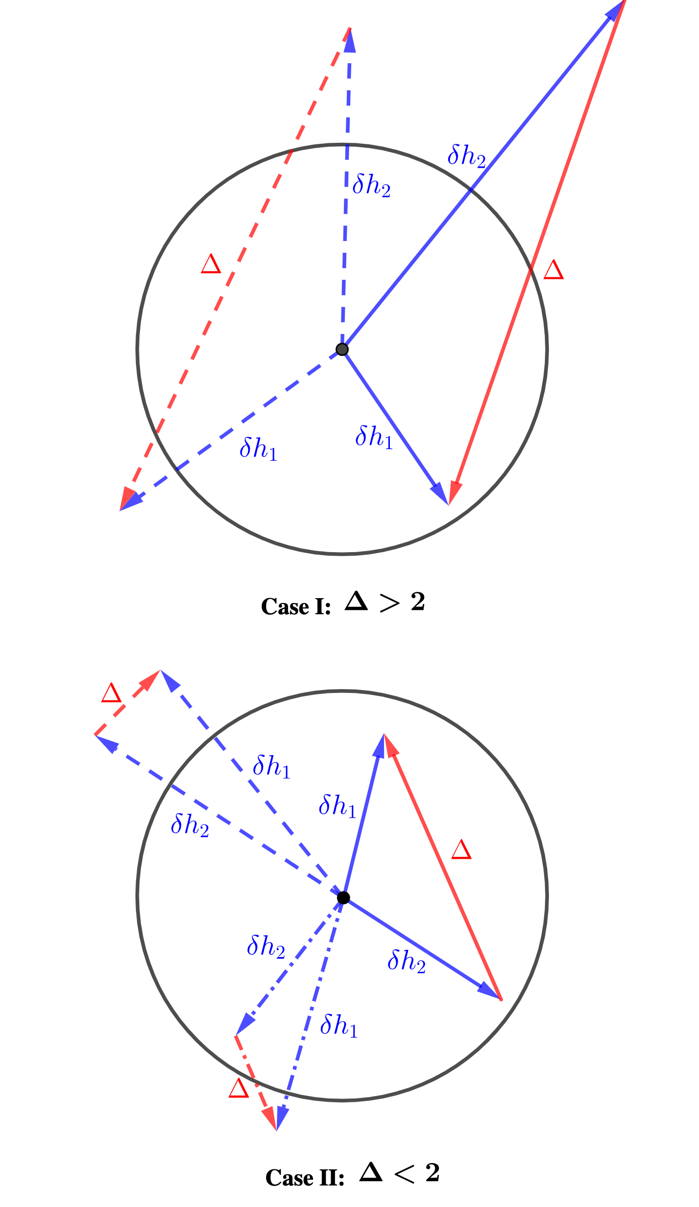
Eq. 11 is not a strong criterion; it can not tell which waveform causes the violation (case I), and may miss some waveform errors (case II). Despite this, we suppose it still gives certain information about the correctness of waveform modeling. If , the waveform pair should become less reliable; if , the systematic errors in waveform models should not be neglected as it is highly possible that either of the waveforms is accurate, or one of them has seriously deviated. If , no evidence of waveform inaccuracy is found by this approach, although we could not exclude the possibility that two waveforms have large but similar errors. The advantage of this method is that it can be performed everywhere in the parameter space, as long as waveform models work in that region.
Eq.11 can be extended to a detector network by defining inner product between matrices (whose elements are frequency series):
| (12) |
where is an matrix, is an matrix and the result is an matrix. The signal of the network can be denoted as a column vector , where superscript denotes the k-th detector and is the number of detectors in the network. We can also subtract two waveform models, and define . The norm of can be calculated
| (13) | ||||
where are the antenna response functions of the k-th detector. In practice, we can weight the by the number of detectors:
| (14) |
so that the will have an upper limit of 2 if the waveforms are both accurate enough.
II.2 Assessment at fixed SNR
The two accuracy standards we proposed, Eq. 11 and Eq. 14, are related to the SNR, as the length of is proportional to the amplitude of GWs. It is reasonable that the higher the SNR is, the easier it is for detectors to distinguish different waveforms, and the more important systematic errors will be in data analysis. However, SNR depends on not only intrinsic parameters, but also extrinsic parameters that trivially modulate the amplitude. It is the phase evolution that is critical to reveal physical properties of the source, and is the intrinsic characteristic of a GW waveform McWilliams et al. 2010 We therefore normalize the with SNR to eliminate the impacts from amplitudes. The optimal SNR is defined as Finn 1992, which is also proportional to the amplitude of GWs like . Thus we have . In fact, we have two waveforms to calculate . The normalization factor is chosen as the geometric mean of SNRs from two waveforms, i.e., . Take Eq. 11 as an example, the normalized is
| (15) | ||||
and we simply have
| (16) |
Eq. 16 can be used to evaluate waveform accuracy at a fixed SNR. Note the threshold of is always 2.
The normalized can be related to the current waveform evaluation variable, overlap , which is defined as
| (17) |
where means the real part. is between 0 and 1, the higher value represents higher similarities between waveforms and . One can define mismatch . Overlap (or the equivalent mismatch) is widely used to assess the correctness of GW waveforms. The state-of-art models of IMRPhenom and SEOBNR families can achieve mismatches between and compared with NR simulations Pratten et al. 2021; Ossokine et al. 2020, with precession effects and higher modes being taken into consideration. Overlap between two waveform models and the length of normalized waveform difference have the following relation:
| (18) |
where . will decrease with the increase of overlap, and a pair of identical waveforms give and .
We should mention that the inner product in the calculation of waveform difference (as well as overlap Kumar et al. 2016), should be minimized (or, for overlap, maximized) over an arbitrary phase and time shift , in order to eliminate the kinematical difference between models Damour et al. 2011. Considering the sensitive frequency band of current GW detectors, the inner product is integrated from 20 Hz to 2048 Hz throughout this paper.
III Applications
In this section we will apply the accuracy standard Eq. 14 and Eq. 16 to GW waveforms from 3 types of compact binary coalescence: BBH, NSBH, and BNS. We employ the assessment on the GWTC parameter estimation samples and parameter grids we generate; the former aims to investigate whether faulty waveforms were used in GW data analysis and possible systematic error caused by waveform errors, while the latter explores waveforms’ performances in different regions of the parameter space. Throughout this paper, we ignore the calibration error, which can cause our waveforms to be slightly different from those used in GWTC-3 and GWTC-2.1 parameter estimation. The calibration error is typically degrees in phase and % in amplitude Sun et al. 2020, and it acts on both waveform models, so ignoring it will not have large impacts on our results.
III.1 BBH waveforms
BBH mergers are the most frequent GW events at this stage: Among all 91 GW candidates (36 in GWTC-3 Abbott et al. 2021b, 44 in GWTC-2.1 The LIGO Scientific Collaboration and The Virgo Collaboration 2021 and 11 in GWTC-1 LIGO Scientific Collaboration and Virgo Collaboration 2019), over 80 of them are confirmed to be BBH events. In the latest data release from LIGO-Virgo-KAGRA (LVK) collaboration, waveform models IMRPhenomXPHM and SEOBNRv4PHM are used for analysis of all the BBH events, including re-analysis of GWTC-1 events published in GWTC-2.1. Due to the low SNR of current NSBH events, the resolution of tidal deformability is poor and no strong sign of matter effects is revealed in data analysis. Besides, higher modes and spin precession effects are more important than matter effects for waveform modeling of NSBHs Abbott et al. 2021d, so IMRPhenomXPHM and SEOBNRv4PHM are also employed on NSBH events to extract physical information.
For all the 89 BBH and NSBH events, we use the cosmologically reweighted parameter estimation posterior samples from GWTC-3 and GWTC-2.1 data release and calculate (Eq. 14 ) of the waveform models mentioned above. We use the mixture of IMRPhenomXPHM and SEOBNRv4PHM samples in most events, but in some events SEOBNRv4PHM samples are not provided The LIGO Scientific Collaboration and The Virgo Collaboration 2021, so we use IMRPhenomXPHM samples to calculate between IMRPhenomXPHM and SEOBNRv4PHM. Samples we use are the same as GWTC-3 Abbott et al. 2021b and GWTC-2.1 The LIGO Scientific Collaboration and The Virgo Collaboration 2021. For each sample, we generate the waveform (including the detector response) for both models, then apply a time and phase shift on one of them to minimize Eq. 14. The minimized is the waveform difference we refer to in the following discussion.
When is greater than 2 at a sampling point, it implies the difference between IMRPhenomXPHM and SEOBNRv4PHM is so large at this point that they could not both be accurate enough. Furthermore, the difference in waveform will induce a difference in likelihood, and therefore has the potential to affect the results of a parameter estimation algorithm. This yields a systematic difference in parameter estimates, and so the results from different waveform models may not coincide. Therefore, in addition to , we also calculate Jensen–Shannon (J-S) divergence between IMRPhenomXPHM samples and SEOBNRv4PHM samples (if available). The J-S divergence is a measurement of the similarity between two probability distributions and is used in GWTC-2 Abbott et al. 2021a. The greater it is, the greater the difference between the two distributions and there may be potential systematic errors in the data analysis. Since the J-S divergence for samples from a distribution is easiest to evaluate in one dimension, we choose the greatest J-S divergence among samples for the following parameters: mass ratio , chirp mass , effective spin and effective precession spin as a measurement of inconsistency of posterior samples, for they are the major physical parameters to be studied. We use gaussian_kde in SciPy to estimate probability density functions. The base of J-S divergence is chosen to be 2, so that the divergence ranges between 0 and 1.
The full results of the 89 BBH and NSBH events are showed splitly in Tab. 1 and Tab. 2 in App. A for reference. We list the basic information of each event, including some source parameters and network SNR, and statistics we construct, including mean value of , normalized (which equals to ), fraction of samples, and the J-S divergence. We highlight some points in the rest of this subsection.
III.1.1 Overall accuracy
We show the relations between the waveform difference of different events and SNR in Fig. 2, in which each point represents a GW event. We find every event has samples that can not meet the requirement (left panel), but most events have mean around 2 (right panel). This means some waveform pairs used in data analysis can pass (and are near the edge of) our accuracy standard, but violations exist. We could not identify whether one or both waveform models is inaccurate. Later in Sec. III.1.3 we will show it is the samples with large spin or small mass ratio or edge-on inclination that contribute to fraction. Overall speaking, considering that the violations are generally not strong, we conclude that the current waveform accuracy is around the edge of our assessment standard for the current detector sensitivity which makes detections of SNRs ranging from to .
Although the properties of GW sources differ, there is a tendency that large SNR events are more likely to have greater waveform difference (as expected by Eq. 16), and have fewer samples that meet the requirement. This emphasizes the importance of waveform modeling for future GW detections, in which the SNR can reach hundreds to thousands. We can also make a rough estimation of waveform accuracy requirements for future detectors. The mismatch with the “true” waveform is widely-used to assess the waveform accuracy, and the relation between and can be derived with Eqs. 16 and 18:
| (19) |
Eq. 19 gives the mismatch between two waveform models, but limited by the triangle inequality, the mismatch between models should be at the same order of magnitude as the mismatch between a model and the real waveform , under the assumption that both models are well-calibrated by high precision waveforms like NR simulation. From our previous discussion we know the is around the edge of its upper limit under the current detector sensitivity. If we assume is of the same range for future detectors, and SNR is roughly 30–100 times higher, we can determine that the mismatch should decrease 3–4 orders of magnitude. This is consistent with the results reported in Ref. Pürrer and Haster 2020.
III.1.2 Impact on parameter estimation
From previous discussions, the waveforms generated by posterior samples of GWTC-3 and GTWC-2.1 are mostly within the waveform difference bound, yet there are some exceptions. Seven GW events have more than 60% posterior samples violating the standard, which means the difference of two waveform models might be too large to ensure their accuracies. The difference of waveforms may result in difference in parameter estimation, indicating systematic errors Williamson et al. 2017; Pürrer and Haster 2020; Cutler and Vallisneri 2007.
We show the relation between waveform difference and posterior sample consistency (maximum J-S divergence) in Fig. 3, where we can see a weak tendency that events with large waveform difference are more likely to have large J-S divergence, i.e., difference in waveform models may lead to inconsistency in parameter estimation. Particularly, when the fraction of samples is below 40%, the maximum J-S divergence would be greater than the majority of the GW events. This coincides with our expectation.
Bottom three rows: We show some examples of inconsistent posterior samples; the parameter name and event name are shown in the plots.
However, the inverse statement is not necessarily true. When most posterior samples meet our accuracy standard, it is also possible that two waveform models give inconsistent results. In fact, the waveform error is not the only factor that causes two sets of posterior samples to differ. The behavior of samplers or packages (bilby Ashton et al. 2019 vs RIFT Lange et al. 2018) and the prior choice (such as high-spin and low-spin prior for neutron stars Abbott et al. 2019) can both influence the consistency between the two posterior samples, although the latter one is not involved in our analysis. Even if we exclude these factors in a full Bayesian analysis, theoretically, it is the combination of waveform gradients, covariance matrices and waveform difference that contributes to systematic errors in parameter estimation Cutler and Vallisneri 2007, not just waveform difference. Besides, we use the maximum J-S divergence as the measurement of posterior difference, which might be influenced when the parameter estimation does not work efficiently on some specific parameters. The last row in Fig. 3 shows such cases. This makes the correlation between posterior sample consistency and waveform difference more statistically dispersed.
In the last three rows of Fig. 3, we give some examples of inconsistent posterior samples. GW200129_065458 has the largest J-S divergence among GWTC-3 events, and GW190412_053044 has the largest J-S divergence among GWTC-2.1 events. The posterior sample inconsistencies of the two events are also reported in GWTC-3 Abbott et al. 2021b and GWTC-2.1 The LIGO Scientific Collaboration and The Virgo Collaboration 2021. In both events, the result with IMRPhenomXPHM suggests the possibility of a low mass ratio binary, while that with SEOBNRv4PHM does not. GW191219_163120 is the lowest mass ratio detection to-date. Its estimated mass ratio is out of the calibration range of waveform models, so potential systematic error may lie in its data analysis Abbott et al. 2021b. In our analysis, GW191219_163120 does have less posterior samples that pass our assessment than most other events, but it is not the worst one. Besides, its high SNR (26.8) also contributes to waveform difference: its waveform difference becomes small after normalization. This might be caused by the small spins indicated by parameter estimation. Therefore, we suppose the waveform modelling is not that problematic in the low mass ratio and small spin region, but its high SNR reduces model waveform accuracy. We show its estimation of effective precession spin in Fig. 3, in which we see result of IMRPhenomXPHM supports high precession effects in this binary system, while result of SEOBNRv4PHM prefers lower precession effects. GW191109_010717 produces the largest waveform difference in our analysis. In a later section III.1.3 we will illustrate it might be caused by its special spin effects and higher modes. We show its estimation of effective spin in Fig. 3: results from two waveform models show different multimodality. We also give examples which do not significantly violate our accuracy standard but have inconsistent posterior samples: GW190930_133541 and GW190708_232457. Their results from IMRPhenomXPHM seem unable to find the most probable mass ratio. There are six events having this behaviour in GWTC-2.1, as labeled by red circles in Fig. 3. Further investigation is needed, but this is beyond the scope of this work.
Since most posterior samples in this analysis satisfy or just slightly violate our accuracy standard, and samples from two waveform models, generated by different samplers and packages, are mixed as the final results to counterbalance systematic errors, we suppose the waveform modelling error will not induce significant systematic error in data analysis for current detector sensitivity at the population level, while some special events still need further investigation.
III.1.3 Waveform difference in different parameter regions
In Sec III.1, from the angle of data analysis, we discussed SNR’s impact on waveform accuracy. What is more physically interesting is how the waveform accuracy varies with intrinsic properties of the GW source. It is plausible that model accuracy decreases when the system includes some complex processes, such as a highly asymmetric mass ratio, high spin effects, high eccentricity and so forth. Accuracy may also drop when the contributions from higher modes increase, which usually happens to edge-on binaries Biscoveanu et al. 2021; Varma and Ajith 2017; Colleoni et al. 2021.
We plot posterior samples of selected events and highlight the samples whose waveform difference is greater than 2 in Fig. 4. In the nearly equal mass region and small spin region, IMRPhenomXPHM and SEOBNRv4PHM agree with each other and have waveform difference less than 2. However, when mass ratio deviates from , or when spin parameters deviates from , the waveform difference grows and the waveform pair fails to pass the accuracy standard. For extrinsic parameters, we find that the waveform difference is largest when inclination angle for precessing systems is close to . We attribute this to two causes: the contribution of higher modes increases when the source is egde-on, and the amplitude modulations caused by precession become increasingly visible, magnifying differences in the way precession is modelled Vitale et al. 2014; Varma and Ajith 2017; Fairhurst et al. 2020; Colleoni et al. 2021; Biscoveanu et al. 2021; Krishnendu and Ohme 2022. This is the reason why events like GW191109_010717 have a small fraction of posterior samples that pass the accuracy standard: estimations of their parameters mainly lead to low mass ratio, high spin regions or edge-on regions.
We then perform simulations of BBH events on the design sensitivity of Advanced LIGO Abbott and et al 2020. We set the primary mass at , and mass ratio at and . The spin of each component is randomly generated: spin magnitude is uniformly distributed between 0 and 1, and spin direction is isotropic. Inclination angle is isotropic as well. We neglect detector response functions and only include plus polarization here, which will not change our qualitative conclusions. For each mass ratio we simulate 6000 BBH events and calculate the waveform difference between IMRPhenomXPHM and SEOBNRv4PHM. Since waveform difference is proportional to SNR, we introduce a SNR threshold above which will be greater than 2. In Fig. 5, we plot the distributions of simulation parameters in the style of corner plot for different mass ratios, and the corresponding SNR thresholds in colors. We find the SNR threshold can reach 30 in the low spin and face-on region, but gradually drops below as the spin parameters increase or tends to . The change in mass ratio has the same effect, can reach at a smaller spin if the mass ratio is low. However, we find the simulations can achieve high SNR threshold for low spin face-on sources, while high-spin or edge-on simulations are more likely to produce low SNR thresholds regardless of the mass ratio. Therefore, for current waveform modeling, spin effects and higher modes may need more improvements than low mass ratio cases. This coincides with our calculation on the asymmetric mass ratio but small spin event GW191219_163120. The disagreement in high-spin CBC waveforms and its impact on parameter estimation is also reported in Ref. Williamson et al. 2017.
Our simulation is consistent with the calculation for real events. Given GW events with SNRs ranging from 8 to 30 (for current detector sensitivity), those generated by nearly equal mass systems or low spin systems would have more samples, while the other events’ posterior samples mostly fail our test, like GW191109_010717. Using the same method in Sec. III.1.1 and comparing current SNR threshold with expected SNR of 3rd generation GW detectors, we can also conclude that, in general, the waveform accuracy should be improved for 3 to 4 orders of magnitude. However, for high spin and low mass ratio regions, as well as higher modes, the current waveform models may need more improvements. To calibrate waveform models, these regions might be where NR simulations are most needed for future waveform modelling.


III.2 NSBH and BNS waveforms
NSBH and BNS events are much less frequent than BBH events so far - only three events are generally considered as NSBH candidates: GW191219_163120, GW200105_162426, and GW200115_042309, and two are considered as BNS events: GW170817 and GW190425_081805. Due to the complexity of these systems (e.g., highly asymmetric mass ratio, eccentricity for NSBH binaries, and matter effects for both types), some physical effects are yet to be included in their waveform models. Current NSBH waveform models of IMRPhenom and SEOBNR familes, IMRPhenomNSBH and SEOBNRv4_ROM_NRTidalv2_NSBH Pannarale et al. 2015, are calibrated by non-spinning neutron star simulations and only allow aligned spins. For current BNS models, IMRPhenomPv2_NRTidalv2 supports precessing spins while SEOBNRv4T_surrogate only supports aligned spins. Recent works have made TEOBResumS able to generate waveforms for precessing BNS systems with higher modes Gamba et al. 2021b , as well as waveforms for eccentric BNS systems Chiaramello and Nagar 2020, but they have not been applied to the GWTC-2.1 and -3.
For the three NSBH events, we calculate the of their posterior samples generated by IMRPhenomNSBH and SEOBNRv4_ROM_NRTidalv2_NSBH. The fraction of samples are and for GW191219_163120, GW200105_162426, and GW200115_042309, respectively. Low SNR of these three events may contribute to the small waveform differences, but compared with the BBH events, lacking of precession effects and higher modes should be the decisive factors that make the waveform pair coincide, and it does not necessarily mean these models can describe general NSBH systems with high accuracy. As for BNS events, IMRPhenomPv2_NRTidalv2 is the only model used in GWTC-2.1 and -3 that includes precession effects, it is not feasible to compare waveform difference of its posterior samples with others. Hence we do not include calculation of BNS waveforms for real events in this work.
We perform simulations for NSBH and BNS systems respectively. For NSBH waveform models, we assume zero spin and secondary mass of . We change mass ratio between and , and tidal deformability parameter between and . For BNS, we assume the two neutron stars are exactly the same: same mass , same tidal deformability parameter and spin. Then we change spin magnitude between and , and tidal deformability parameter between and . We assume zero inclination for both systems. The results are shown in Fig. 6.

Right panel: Simulations of BNS binaries in the tidal deformability - effective spin plane. We assume both neutron stars are and they have the same spin and tidal deformability parameter. Colors represent SNR threshold for IMRPhenomPv2_NRTidalv2 and SEOBNRv4T_surrogate.
We find the main disagreement for NSBH waveform models lies in mass ratio, as Fig. 6 shows the waveform difference drops with but is insensitive to the tidal deformability parameter of the neutron star. The latter is because both approximants use the NRTidalv2 Dietrich et al. 2019 phase description to model the matter effects. SNR threshold can drop below 5 when is small, but all the three NSBH candidates have SNRs lower than the thresholds indicated in the corresponding regions in Fig. 6. Note we assume zero spin in this simulation, but non-zero spin samples exist in the three NSBH candidates and would make extra contributions to waveform difference. Therefore, they still have a small fraction of samples. Given the SNR threshold in this simulation, NSBH waveform model accuracies (in terms of the mismatch from real waveform) also need an improvement of 3–4 orders of magnitude for future detection, leaving aside the unincluded physical effects.
As for BNS waveforms IMRPhenomPv2_NRTidalv2 and SEOBNRv4T_surrogate, we change values of and spin magnitude. We assume both components have the same aligned spin and mass, so the individual spin magnitude is equal to the effective spin. We find two waveform models agree with each other quite well in the , region, with SNR thresholds up to 100. This is the region that coincides with our current understanding of neutron stars. However, when spin increases, the SNR threshold can drop below 20. This also implies accuracy of future waveform models should be improved by several orders of magnitude.
We do not discuss further about NSBH and BNS waveform models, for we suppose the number of real events is not enough for us to perform analysis on the population level, and further work on precession, higher modes, and even eccentricity should be done for more NSBH and BNS waveform models.
IV Conclusions
In this work, we developed a diagnostic test for the presence of waveform mismodelling. This extends the work of Ref. Lindblom et al. 2008 to realistic analyses. While Ref. Lindblom et al. 2008 suggests a waveform model should have error (as a vector) shorter than 1 to be accurate enough, we introduce two waveform models and find their difference should be shorter than 2 if they are both accurate enough. This method frees accuracy evaluation from the unknown true waveform, and it enables the evaluation to be performed in larger, continuous regions in the parameter space: the regions where waveform models can work, rather than where NR simulations are done. We should note that our method can only tell the existence of inaccurate waveform models. It can not tell which one (or both) is (are) inaccurate if the pair fail, or guarantee any accuracy when the pair do not fail. The key idea is: If two models have significant difference, they can not be both accurate enough, but when the difference is small, we can not rule out the possibility that two models are making similar mistakes.
For BBH waveform models, we choose the statr-of-art models from IMRPhenom and SEOBNR family, IMRPhenomXPHM and SEOBNRv4PHM for illustration. We have applied our test to existing parameter estimates from the GWTC-3 and GWTC-2.1 (which used the waveform models mentioned above), and found differences in the results of data analysis from different waveform models. The samples that fail our test are mostly located in the low mass ratio, high spin or egde-on regions in the parameter space, which means waveform models become less reliable in these regions. Our simulations agree with this: the waveform difference between IMRPhenomXPHM and SEOBNRv4PHM can reach the threshold 2 when SNR is less than 10 in high spin regions and edge-on regions; waveform difference increases in low mass ratio region the as well. We also note that spin effects and inclinations (higher modes) are more problematic for waveform modelling than mass ratio. This points out where NR simulations are needed most for future waveform calibration.
We have investigated the correlation between waveform difference and inconsistency of parameter estimation samples given by different waveform models. The latter is measured by the J-S divergence. For the GWTC-3 and GWTC-2.1 posterior samples, we find when the fraction of samples is less than 40%, it is more likely to obtain a J-S divergence larger than most other events, which is a sign of underlying systematic errors caused by waveform error. We also note that the inverse is not necessarily true, as the waveform model is not the only factor that can influence the generation of posterior samples, but nonetheless it is always helpful to have one of the factors checked. Since multi-waveform analysis is becoming a standard way of reducing systematic errors in parameter estimation of GW sources, we suggest that waveform difference analysis can be used as a real-time quantitative check in the parameter estimation workflow.
For NSBH waveforms, we select IMRPhenomNSBH and SEOBNRv4_ROM_NRTidalv2_NSBH, the two models used in GWTC-3 and GWTC-2.1 parameter estimation. The posterior samples of the 3 NSBH candidates have small NSBH waveform difference compared to BBH waveforms. We credit this to the fact that these waveform models do not include non-aligned spins or higher modes as BBH waveforms. As expected, we find waveform difference increase when mass ratio decreases in our simulation. The SNR threshold drops below 10 when mass ratio is less than 0.05, indicating that more calibrations are needed for this region, leaving aside the lack of some other physical effects.
For BNS waveforms, we have not applied our test on real events samples, for only IMRPhenomPv2_NRTidalv2 is used in GWTC-2.1 and -3 data analysis, and we could not find another comparable model to be paired with it. We simulate aligned spin BNSs for IMRPhenomPv2_NRTidalv2 and SEOBNRv4T_surrogate instead. We find the systematic differences between the approximants we examined are small in the region where , and , which should be the case for our current understanding of neutron stars. However, there are some differences when where the waveforms appear to diverge again. In the high spin regions, the SNR threshold drops below 20, which can not meet future high SNR detections.
The waveform difference is related to the widely used overlap (or mismatch) through Eqs. 18 and 19. If we assume two models are well calibrated and have comparable errors, we can give a rough estimate of future waveform accuracy requirement. This complements previous works on waveform accuracy Pürrer and Haster 2020. Looking at the SNR thresholds for the three types of waveforms, we know the current waveform accuracy is not enough for future high SNR detections where SNR can reaches up to 1000. The mismatch from the real waveform needed to be reduced by at least 3 orders of magnitude. This is consistent with previous work.
Finally, this method can be extended to more complex GW waveform models for future GW detection, such as waveforms including eccentricity. We can perform this analysis as long as there are at least two waveform models with the similar accuracy and which include the same physical parameters. Our method can work beyond the NR calibration range, thus it can be efficient way to study the waveform models’ extrapolation performance. This may also be a guide of where NR simulations are most needed in the parameter space.
Acknowledgements.
The authors would like to thank Daniel Williams, Michael Pürrer, Christopher Berry, Ik Siong Heng, Rossella Gamba and Jacob Lange for helpful discussions and suggestions. Daniel also helped us use the GWTC-3 and GWTC-2.1 PE data release. The authors are grateful for computational resources provided by the LIGO Lab at Caltech which is supported by National Science Foundation Grants PHY-0757058 and PHY-0823459. QH is supported by CSC. JV is supported by STFC grant ST/V005634/1.Appendix A Full results of BBH waveform in GWTC-3 and GWTC-2.1
| Event name | SNR | Mean | Fraction | Max J-S Div. | ||||||
|---|---|---|---|---|---|---|---|---|---|---|
| GW150914_095045 | 24.4 | 2.0 | 0.08 | 0.59 | 0.069 | |||||
| GW151012_095443 | 10 | 1.33 | 0.13 | 0.81 | 0.023 | |||||
| GW151226_033853 | 13.1 | 2.39 | 0.18 | 0.54 | N/A | |||||
| GW170104_101158 | 13 | 1.28 | 0.1 | 0.88 | 0.01 | |||||
| GW170608_020116 | 14.9 | 1.43 | 0.1 | 0.86 | 0.051 | |||||
| GW170729_185629 | 10.8 | 2.08 | 0.19 | 0.54 | 0.037 | |||||
| GW170809_082821 | 12.4 | 1.14 | 0.09 | 0.91 | 0.037 | |||||
| GW170814_103043 | 15.9 | 1.31 | 0.08 | 0.88 | 0.062 | |||||
| GW170818_022509 | 11.3 | 1.06 | 0.09 | 0.96 | 0.015 | |||||
| GW170823_131358 | 11.5 | 1.83 | 0.16 | 0.64 | 0.019 | |||||
| GW190408_181802 | 14.4 | 1.05 | 0.07 | 0.94 | 0.006 | |||||
| GW190412_053044 | 18.2 | 2.86 | 0.16 | 0.25 | 0.45 | |||||
| GW190413_052954 | 8.5 | 1.13 | 0.13 | 0.88 | N/A | |||||
| GW190413_134308 | 10.3 | 1.57 | 0.15 | 0.71 | N/A | |||||
| GW190421_213856 | 9.7 | 1.59 | 0.16 | 0.73 | N/A | |||||
| GW190503_185404 | 12.2 | 1.55 | 0.13 | 0.74 | 0.013 | |||||
| GW190512_180714 | 12.2 | 1.3 | 0.11 | 0.85 | 0.036 | |||||
| GW190513_205428 | 12.3 | 1.64 | 0.13 | 0.7 | 0.048 | |||||
| GW190514_065416 | 8.3 | 1.44 | 0.17 | 0.78 | 0.013 | |||||
| GW190517_055101 | 10.8 | 2.04 | 0.19 | 0.61 | 0.141 | |||||
| GW190519_153544 | 12.4 | 2.81 | 0.23 | 0.24 | 0.066 | |||||
| GW190521_030229 | 13.3 | 3.24 | 0.24 | 0.35 | N/A | |||||
| GW190521_074359 | 24.4 | 3.6 | 0.15 | 0.13 | 0.153 | |||||
| GW190527_092055 | 8.7 | 1.29 | 0.15 | 0.85 | 0.161 | |||||
| GW190602_175927 | 12.3 | 1.95 | 0.16 | 0.6 | N/A | |||||
| GW190620_030421 | 10.9 | 2.1 | 0.19 | 0.52 | 0.049 | |||||
| GW190630_185205 | 15.2 | 1.55 | 0.1 | 0.76 | 0.032 | |||||
| GW190701_203306 | 11.7 | 0.95 | 0.08 | 0.95 | 0.007 | |||||
| GW190706_222641 | 12.5 | 3.06 | 0.24 | 0.26 | 0.093 | |||||
| GW190707_093326 | 13.2 | 1.23 | 0.09 | 0.93 | 0.219 | |||||
| GW190708_232457 | 13.1 | 1.14 | 0.09 | 0.94 | 0.424 | |||||
| GW190719_215514 | 8 | 1.41 | 0.18 | 0.79 | N/A | |||||
| GW190720_000836 | 11.5 | 0.86 | 0.08 | 0.97 | 0.14 | |||||
| GW190727_060333 | 12.1 | 1.37 | 0.11 | 0.82 | 0.017 | |||||
| GW190728_064510 | 13.4 | 1.16 | 0.09 | 0.89 | 0.048 | |||||
| GW190731_140936 | 8.5 | 1.13 | 0.13 | 0.89 | 0.031 | |||||
| GW190803_022701 | 9.1 | 0.87 | 0.1 | 0.96 | N/A | |||||
| GW190814_211039 | 22.2 | 2.54 | 0.11 | 0.49 | N/A | |||||
| GW190828_063405 | 16.3 | 1.31 | 0.08 | 0.86 | N/A | |||||
| GW190828_065509 | 11.1 | 1.69 | 0.15 | 0.68 | N/A | |||||
| GW190910_112807 | 13.4 | 2.25 | 0.17 | 0.47 | 0.011 | |||||
| GW190915_235702 | 13 | 1.63 | 0.13 | 0.69 | 0.01 | |||||
| GW190924_021846 | 13 | 1.13 | 0.09 | 0.92 | 0.152 | |||||
| GW190929_012149 | 10.1 | 2.22 | 0.22 | 0.47 | N/A | |||||
| GW190930_133541 | 10.1 | 1.2 | 0.12 | 0.87 | 0.377 |
| Event name | SNR | Mean | Fraction | Max J-S Div. | ||||||
|---|---|---|---|---|---|---|---|---|---|---|
| GW190403_051519 | 8 | 1.62 | 0.2 | 0.72 | 0.052 | |||||
| GW190426_190642 | 9.6 | 1.55 | 0.16 | 0.74 | N/A | |||||
| GW190725_174728 | 9.1 | 1.04 | 0.11 | 0.92 | N/A | |||||
| GW190805_211137 | 8.3 | 1.3 | 0.16 | 0.84 | 0.014 | |||||
| GW190916_200658 | 8.2 | 1.14 | 0.14 | 0.89 | 0.004 | |||||
| GW190917_114630 | 9.5 | 1.06 | 0.11 | 0.93 | N/A | |||||
| GW190925_232845 | 9.9 | 1.09 | 0.11 | 0.91 | 0.008 | |||||
| GW190926_050336 | 9 | 1.49 | 0.17 | 0.74 | N/A | |||||
| GW191103_012549 | 8.9 | 1.01 | 0.11 | 0.92 | 0.012 | |||||
| GW191105_143521 | 9.7 | 0.77 | 0.08 | 0.99 | 0.02 | |||||
| GW191109_010717 | 17.3 | 5.8 | 0.34 | 0.1 | 0.086 | |||||
| GW191113_071753 | 7.9 | 1.68 | 0.21 | 0.67 | 0.048 | |||||
| GW191126_115259 | 8.3 | 1.14 | 0.14 | 0.89 | 0.01 | |||||
| GW191127_050227 | 9.2 | 1.9 | 0.21 | 0.6 | 0.089 | |||||
| GW191129_134029 | 13.1 | 1.34 | 0.1 | 0.87 | 0.033 | |||||
| GW191204_110529 | 8.8 | 1.59 | 0.18 | 0.72 | 0.027 | |||||
| GW191204_171526 | 17.5 | 1.67 | 0.1 | 0.73 | 0.045 | |||||
| GW191215_223052 | 11.2 | 1.06 | 0.09 | 0.95 | 0.01 | |||||
| GW191216_213338 | 18.6 | 1.93 | 0.1 | 0.62 | 0.06 | |||||
| GW191219_163120 | 9.1 | 2.51 | 0.28 | 0.34 | 0.13 | |||||
| GW191222_033537 | 12.5 | 2.02 | 0.16 | 0.57 | 0.017 | |||||
| GW191230_180458 | 10.4 | 1.17 | 0.11 | 0.88 | 0.011 | |||||
| GW200105_162426 | 13.7 | 1.47 | 0.11 | 0.79 | 0.162 | |||||
| GW200112_155838 | 19.8 | 1.63 | 0.08 | 0.73 | 0.061 | |||||
| GW200115_042309 | 11.3 | 1.35 | 0.12 | 0.81 | 0.096 | |||||
| GW200128_022011 | 10.6 | 2.12 | 0.2 | 0.55 | 0.09 | |||||
| GW200129_065458 | 26.8 | 2.33 | 0.09 | 0.47 | 0.425 | |||||
| GW200202_154313 | 10.8 | 0.74 | 0.07 | 0.99 | 0.025 | |||||
| GW200208_130117 | 10.8 | 1.19 | 0.11 | 0.87 | 0.017 | |||||
| GW200208_222617 | 7.4 | 1.91 | 0.26 | 0.6 | 0.171 | |||||
| GW200209_085452 | 9.6 | 1.29 | 0.13 | 0.83 | 0.014 | |||||
| GW200210_092254 | 8.4 | 1.2 | 0.14 | 0.88 | 0.06 | |||||
| GW200216_220804 | 8.1 | 1.32 | 0.16 | 0.82 | 0.006 | |||||
| GW200219_094415 | 10.7 | 1.61 | 0.15 | 0.71 | 0.017 | |||||
| GW200220_061928 | 7.2 | 1.2 | 0.17 | 0.87 | 0.022 | |||||
| GW200220_124850 | 8.5 | 1.72 | 0.2 | 0.68 | 0.007 | |||||
| GW200224_222234 | 20 | 2.26 | 0.11 | 0.52 | 0.022 | |||||
| GW200225_060421 | 12.5 | 1.43 | 0.11 | 0.8 | 0.015 | |||||
| GW200302_015811 | 10.8 | 2.13 | 0.2 | 0.51 | 0.054 | |||||
| GW200306_093714 | 7.8 | 1.33 | 0.17 | 0.82 | 0.013 | |||||
| GW200308_173609 | 7.1 | 1.1 | 0.15 | 0.89 | 0.054 | |||||
| GW200311_115853 | 17.8 | 1.27 | 0.07 | 0.87 | 0.026 | |||||
| GW200316_215756 | 10.3 | 1.08 | 0.1 | 0.9 | 0.082 | |||||
| GW200322_091133 | 6 | 0.87 | 0.14 | 0.94 | 0.059 |
References
- LIGO Scientific Collaboration and Virgo Collaboration (2019) LIGO Scientific Collaboration and Virgo Collaboration, GWTC-1: A Gravitational-Wave Transient Catalog of Compact Binary Mergers Observed by LIGO and Virgo during the First and Second Observing Runs, Physical Review X 9, 031040 (2019).
- Abbott et al. (2021a) R. Abbott et al., GWTC-2: Compact Binary Coalescences Observed by LIGO and Virgo during the First Half of the Third Observing Run, Physical Review X 11, 1–54 (2021a).
- Abbott et al. (2021b) R. Abbott et al., GWTC-3: Compact Binary Coalescences Observed by LIGO and Virgo During the Second Part of the Third Observing Run (2021b), arXiv:2111.03606 .
- The LIGO Scientific Collaboration and The Virgo Collaboration (2021) The LIGO Scientific Collaboration and The Virgo Collaboration, GWTC-2.1: Deep Extended Catalog of Compact Binary Coalescences Observed by LIGO and Virgo During the First Half of the Third Observing Run (2021), arXiv:2108.01045 [gr-qc] .
- Nitz et al. (2019) A. H. Nitz, C. Capano, A. B. Nielsen, S. Reyes, R. White, D. A. Brown, and B. Krishnan, 1-OGC: The First Open Gravitational-wave Catalog of Binary Mergers from Analysis of Public Advanced LIGO Data, The Astrophysical Journal 872, 195 (2019).
- Nitz et al. (2020) A. H. Nitz, T. Dent, G. S. Davies, S. Kumar, C. D. Capano, I. Harry, S. Mozzon, L. Nuttall, A. Lundgren, and M. Tápai, 2-OGC: Open Gravitational-wave Catalog of Binary Mergers from Analysis of Public Advanced LIGO and Virgo Data, The Astrophysical Journal 891, 123 (2020).
- Nitz et al. (2021a) A. H. Nitz, C. D. Capano, S. Kumar, Y.-F. Wang, S. Kastha, M. Schäfer, R. Dhurkunde, and M. Cabero, 3-OGC: Catalog of gravitational waves from compact-binary mergers, The Astrophysical Journal 922, 76 (2021a), arXiv:2105.09151 .
- Nitz et al. (2021b) A. H. Nitz, S. Kumar, Y.-F. Wang, S. Kastha, S. Wu, M. Schäfer, R. Dhurkunde, and C. D. Capano, 4-OGC: Catalog of gravitational waves from compact-binary mergers, arXiv (2021b), arXiv:2112.06878 .
- Zackay et al. (2021) B. Zackay, L. Dai, T. Venumadhav, J. Roulet, and M. Zaldarriaga, Detecting gravitational waves with disparate detector responses: Two new binary black hole mergers, Physical Review D 104, 10.1103/physrevd.104.063030 (2021).
- Venumadhav et al. (2020) T. Venumadhav, B. Zackay, J. Roulet, L. Dai, and M. Zaldarriaga, New binary black hole mergers in the second observing run of Advanced LIGO and Advanced Virgo, Phys. Rev. D 101, 083030 (2020).
- Venumadhav et al. (2019) T. Venumadhav, B. Zackay, J. Roulet, L. Dai, and M. Zaldarriaga, New search pipeline for compact binary mergers: Results for binary black holes in the first observing run of advanced ligo, Phys. Rev. D 100, 023011 (2019).
- Zackay et al. (2019) B. Zackay, T. Venumadhav, L. Dai, J. Roulet, and M. Zaldarriaga, Highly spinning and aligned binary black hole merger in the advanced ligo first observing run, Phys. Rev. D 100, 023007 (2019).
- Aasi et al. (2015) J. Aasi et al., Advanced LIGO, Classical and Quantum Gravity 32, 074001 (2015), arXiv:1411.4547 .
- Acernese et al. (2015) F. Acernese et al., Advanced Virgo: A 2nd generation interferometric gravitational wave detector, Classical and Quantum Gravity 32, 024001 (2015), arXiv:1408.3978 .
- Allen et al. (2012) B. Allen, W. G. Anderson, P. R. Brady, D. A. Brown, and J. D. E. Creighton, FINDCHIRP: An algorithm for detection of gravitational waves from inspiraling compact binaries, Physical Review D 85, 122006 (2012).
- Veitch et al. (2015) J. Veitch et al., Parameter estimation for compact binaries with ground-based gravitational-wave observations using the LALInference software library, Physical Review D 91, 1–25 (2015).
- Biwer et al. (2019) C. M. Biwer, C. D. Capano, S. De, M. Cabero, D. A. Brown, A. H. Nitz, and V. Raymond, PyCBC inference: A python-based parameter estimation toolkit for compact binary coalescence signals, Publications of the Astronomical Society of the Pacific 131, 10.1088/1538-3873/aaef0b (2019).
- Lange et al. (2018) J. Lange, R. O’Shaughnessy, and M. Rizzo, Rapid and accurate parameter inference for coalescing, precessing compact binaries (2018), arXiv:1805.10457 .
- Ashton et al. (2019) G. Ashton et al., BILBY: A user-friendly Bayesian inference library for gravitational-wave astronomy, Astrophys. J. Suppl. 241, 27 (2019), arXiv:1811.02042 [astro-ph.IM] .
- Lindblom et al. (2008) L. Lindblom, B. J. Owen, and D. A. Brown, Model waveform accuracy standards for gravitational wave data analysis, Physical Review D 78, 1–12 (2008).
- Blanchet (2014) L. Blanchet, Gravitational radiation from post-newtonian sources and inspiralling compact binaries, Living Reviews in Relativity 17, 1–185 (2014).
- Berti et al. (2009) E. Berti, V. Cardoso, and A. O. Starinets, Quasinormal modes of black holes and black branes, Classical and Quantum Gravity 26, 163001 (2009).
- Jani et al. (2016) K. Jani, J. Healy, J. A. Clark, L. London, P. Laguna, and D. Shoemaker, Georgia tech catalog of gravitational waveforms, Classical and Quantum Gravity 33, 1–8 (2016).
- Mroué et al. (2013) A. H. Mroué et al., Catalog of 174 Binary Black Hole Simulations for Gravitational Wave Astronomy, Physical Review Letters 111, 241104 (2013).
- Boyle et al. (2019) M. Boyle et al., The SXS collaboration catalog of binary black hole simulations, Classical and Quantum Gravity 36, 195006 (2019).
- Szilágyi et al. (2015) B. Szilágyi, J. Blackman, A. Buonanno, A. Taracchini, H. P. Pfeiffer, M. A. Scheel, T. Chu, L. E. Kidder, and Y. Pan, Approaching the post-newtonian regime with numerical relativity: A compact-object binary simulation spanning 350 gravitational-wave cycles, Physical Review Letters 115, 10.1103/physrevlett.115.031102 (2015).
- Ajith et al. (2007) P. Ajith et al., A phenomenological template family for black-hole coalescence waveforms, Classical and Quantum Gravity 24, S689 (2007).
- Khan et al. (2016) S. Khan, S. Husa, M. Hannam, F. Ohme, M. Pürrer, X. Jiménez Forteza, and A. Bohé, Frequency-domain gravitational waves from nonprecessing black-hole binaries. II. A phenomenological model for the advanced detector era, Phys. Rev. D 93, 044007 (2016), arXiv:1508.07253 [gr-qc] .
- Pratten et al. (2020) G. Pratten, S. Husa, C. Garcia-Quiros, M. Colleoni, A. Ramos-Buades, H. Estelles, and R. Jaume, Setting the cornerstone for a family of models for gravitational waves from compact binaries: The dominant harmonic for nonprecessing quasicircular black holes, Phys. Rev. D 102, 064001 (2020), arXiv:2001.11412 [gr-qc] .
- García-Quirós et al. (2020) C. García-Quirós, M. Colleoni, S. Husa, H. Estellés, G. Pratten, A. Ramos-Buades, M. Mateu-Lucena, and R. Jaume, Multimode frequency-domain model for the gravitational wave signal from nonprecessing black-hole binaries, Phys. Rev. D 102, 064002 (2020), arXiv:2001.10914 [gr-qc] .
- Pratten et al. (2021) G. Pratten et al., Computationally efficient models for the dominant and subdominant harmonic modes of precessing binary black holes, Physical Review D 103, 104056 (2021).
- Buonanno and Damour (1999) A. Buonanno and T. Damour, Effective one-body approach to general relativistic two-body dynamics, Physical Review D 59, 084006 (1999).
- Damour (2001) T. Damour, Coalescence of two spinning black holes: an effective one-body approach, Phys. Rev. D 64, 124013 (2001), arXiv:gr-qc/0103018 .
- Bohé et al. (2017) A. Bohé et al., Improved effective-one-body model of spinning, nonprecessing binary black holes for the era of gravitational-wave astrophysics with advanced detectors, Phys. Rev. D 95, 044028 (2017), arXiv:1611.03703 [gr-qc] .
- Cotesta et al. (2018) R. Cotesta, A. Buonanno, A. Bohé, A. Taracchini, I. Hinder, and S. Ossokine, Enriching the Symphony of Gravitational Waves from Binary Black Holes by Tuning Higher Harmonics, Phys. Rev. D 98, 084028 (2018), arXiv:1803.10701 [gr-qc] .
- Pan et al. (2014) Y. Pan, A. Buonanno, A. Taracchini, L. E. Kidder, A. H. Mroué, H. P. Pfeiffer, M. A. Scheel, and B. Szilágyi, Inspiral-merger-ringdown waveforms of spinning, precessing black-hole binaries in the effective-one-body formalism, Phys. Rev. D 89, 084006 (2014), arXiv:1307.6232 [gr-qc] .
- Ossokine et al. (2020) S. Ossokine et al., Multipolar effective-one-body waveforms for precessing binary black holes: Construction and validation, Physical Review D 102, 044055 (2020).
- Nagar et al. (2018) A. Nagar et al., Time-domain effective-one-body gravitational waveforms for coalescing compact binaries with nonprecessing spins, tides and self-spin effects, Phys. Rev. D 98, 104052 (2018), arXiv:1806.01772 [gr-qc] .
- Nagar et al. (2020a) A. Nagar, G. Riemenschneider, G. Pratten, P. Rettegno, and F. Messina, Multipolar effective one body waveform model for spin-aligned black hole binaries, Phys. Rev. D 102, 024077 (2020a), arXiv:2001.09082 [gr-qc] .
- Nagar et al. (2020b) A. Nagar, G. Pratten, G. Riemenschneider, and R. Gamba, Multipolar effective one body model for nonspinning black hole binaries, Phys. Rev. D 101, 024041 (2020b), arXiv:1904.09550 [gr-qc] .
- Blackman et al. (2015) J. Blackman, S. E. Field, C. R. Galley, B. Szilágyi, M. A. Scheel, M. Tiglio, and D. A. Hemberger, Fast and Accurate Prediction of Numerical Relativity Waveforms from Binary Black Hole Coalescences Using Surrogate Models, Physical Review Letters 115, 121102 (2015).
- Varma et al. (2019) V. Varma, S. E. Field, M. A. Scheel, J. Blackman, D. Gerosa, L. C. Stein, L. E. Kidder, and H. P. Pfeiffer, Surrogate models for precessing binary black hole simulations with unequal masses, Phys. Rev. Research. 1, 033015 (2019), arXiv:1905.09300 [gr-qc] .
- Williams et al. (2020) D. Williams, I. S. Heng, J. Gair, J. A. Clark, and B. Khamesra, Precessing numerical relativity waveform surrogate model for binary black holes: A Gaussian process regression approach, Physical Review D 101, 10.1103/PhysRevD.101.063011 (2020).
- Field et al. (2014) S. E. Field, C. R. Galley, J. S. Hesthaven, J. Kaye, and M. Tiglio, Fast prediction and evaluation of gravitational waveforms using surrogate models, Phys. Rev. X 4, 031006 (2014), arXiv:1308.3565 [gr-qc] .
- Pürrer (2014) M. Pürrer, Frequency domain reduced order models for gravitational waves from aligned-spin compact binaries, Class. Quant. Grav. 31, 195010 (2014), arXiv:1402.4146 [gr-qc] .
- Abbott et al. (2020a) R. Abbott et al., GW190521: A Binary Black Hole Merger with a Total Mass of 150 M, Physical Review Letters 125, 1–17 (2020a).
- Abbott et al. (2020b) R. Abbott et al., GW190412: Observation of a binary-black-hole coalescence with asymmetric masses, Physical Review D 102, 043015 (2020b).
- Pürrer and Haster (2020) M. Pürrer and C. J. Haster, Gravitational waveform accuracy requirements for future ground-based detectors, Physical Review Research 2, 1–30 (2020).
- Kumar et al. (2016) P. Kumar, T. Chu, H. Fong, H. P. Pfeiffer, M. Boyle, D. A. Hemberger, L. E. Kidder, M. A. Scheel, and B. Szilagyi, Accuracy of binary black hole waveform models for aligned-spin binaries, Physical Review D 93, 1–25 (2016).
- Abbott et al. (2021c) R. Abbott et al. (LIGO Scientific Collaboration, VIRGO Collaboration, KAGRA Collaboration), The population of merging compact binaries inferred using gravitational waves through GWTC-3 (2021c), arXiv:2111.03634 [astro-ph.HE] .
- Hannam et al. (2021) M. Hannam, C. Hoy, J. E. Thompson, S. Fairhurst, and V. Raymond (VIRGO), Measurement of general-relativistic precession in a black-hole binary (2021), arXiv:2112.11300 [gr-qc] .
- Jan et al. (2020) A. Z. Jan, A. B. Yelikar, J. Lange, and R. O’Shaughnessy, Assessing and marginalizing over compact binary coalescence waveform systematics with RIFT, Phys. Rev. D 102, 124069 (2020), arXiv:2011.03571 [gr-qc] .
- Williamson et al. (2017) A. R. Williamson, J. Lange, R. O’Shaughnessy, J. A. Clark, P. Kumar, J. Calderón Bustillo, and J. Veitch, Systematic challenges for future gravitational wave measurements of precessing binary black holes, Phys. Rev. D 96, 124041 (2017), arXiv:1709.03095 [gr-qc] .
- Ferguson et al. (2021) D. Ferguson, K. Jani, P. Laguna, and D. Shoemaker, Assessing the readiness of numerical relativity for LISA and 3G detectors, Physical Review D 104, 044037 (2021).
- Kunert et al. (2022) N. Kunert, P. T. H. Pang, I. Tews, M. W. Coughlin, and T. Dietrich, Quantifying modeling uncertainties when combining multiple gravitational-wave detections from binary neutron star sources, Phys. Rev. D 105, L061301 (2022), arXiv:2110.11835 [astro-ph.HE] .
- Gamba et al. (2021a) R. Gamba, M. Breschi, S. Bernuzzi, M. Agathos, and A. Nagar, Waveform systematics in the gravitational-wave inference of tidal parameters and equation of state from binary neutron-star signals, Phys. Rev. D 103, 124015 (2021a).
- Finn (1992) L. S. Finn, Detection, measurement, and gravitational radiation, Physical Review D 46, 5236 (1992).
- Cutler and Flanagan (1994) C. Cutler and I. E. Flanagan, Gravitational waves from merging compact binaries: How accurately can one extract the binary’s parameters from the inspiral waveform?, Physical Review D 49, 2658 (1994).
- Damour et al. (2011) T. Damour, A. Nagar, and M. Trias, Accuracy and effectualness of closed-form, frequency-domain waveforms for non-spinning black hole binaries, Phys. Rev. D 83, 024006 (2011), arXiv:1009.5998 [gr-qc] .
- Jaranowski et al. (1998) P. Jaranowski, A. Królak, and B. F. Schutz, Data analysis of gravitational-wave signals from spinning neutron stars: The signal and its detection, Physical Review D 58, 063001 (1998).
- Santamaria et al. (2010) L. Santamaria et al., Matching post-Newtonian and numerical relativity waveforms: systematic errors and a new phenomenological model for non-precessing black hole binaries, Phys. Rev. D 82, 064016 (2010), arXiv:1005.3306 [gr-qc] .
- McWilliams et al. (2010) S. T. McWilliams, B. J. Kelly, and J. G. Baker, Observing mergers of non-spinning black-hole binaries, Phys. Rev. D 82, 024014 (2010), arXiv:1004.0961 [gr-qc] .
- Sun et al. (2020) L. Sun et al., Characterization of systematic error in Advanced LIGO calibration, Class. Quant. Grav. 37, 225008 (2020), arXiv:2005.02531 [astro-ph.IM] .
- Abbott et al. (2021d) R. Abbott et al. (LIGO Scientific Collaboration, KAGRA Collaboration, Virgo Collaboration), Observation of Gravitational Waves from Two Neutron Star–Black Hole Coalescences, Astrophys. J. Lett. 915, L5 (2021d), arXiv:2106.15163 [astro-ph.HE] .
- Cutler and Vallisneri (2007) C. Cutler and M. Vallisneri, LISA detections of massive black hole inspirals: Parameter extraction errors due to inaccurate template waveforms, Physical Review D 76, 104018 (2007), arXiv:0707.2982 .
- Abbott et al. (2019) B. P. Abbott et al., Properties of the Binary Neutron Star Merger GW170817, Physical Review X 9, 011001 (2019).
- Biscoveanu et al. (2021) S. Biscoveanu, M. Isi, V. Varma, and S. Vitale, Measuring the spins of heavy binary black holes, Phys. Rev. D 104, 103018 (2021), arXiv:2106.06492 [gr-qc] .
- Varma and Ajith (2017) V. Varma and P. Ajith, Effects of nonquadrupole modes in the detection and parameter estimation of black hole binaries with nonprecessing spins, Phys. Rev. D 96, 124024 (2017), arXiv:1612.05608 [gr-qc] .
- Colleoni et al. (2021) M. Colleoni, M. Mateu-Lucena, H. Estellés, C. García-Quirós, D. Keitel, G. Pratten, A. Ramos-Buades, and S. Husa, Towards the routine use of subdominant harmonics in gravitational-wave inference: Reanalysis of GW190412 with generation X waveform models, Phys. Rev. D 103, 024029 (2021), arXiv:2010.05830 [gr-qc] .
- Vitale et al. (2014) S. Vitale, R. Lynch, J. Veitch, V. Raymond, and R. Sturani, Measuring the spin of black holes in binary systems using gravitational waves, Phys. Rev. Lett. 112, 251101 (2014), arXiv:1403.0129 [gr-qc] .
- Fairhurst et al. (2020) S. Fairhurst, R. Green, C. Hoy, M. Hannam, and A. Muir, Two-harmonic approximation for gravitational waveforms from precessing binaries, Phys. Rev. D 102, 024055 (2020), arXiv:1908.05707 [gr-qc] .
- Krishnendu and Ohme (2022) N. V. Krishnendu and F. Ohme, Interplay of spin-precession and higher harmonics in the parameter estimation of binary black holes, Phys. Rev. D 105, 064012 (2022), arXiv:2110.00766 [gr-qc] .
- Abbott and et al (2020) B. P. Abbott and et al, Prospects for observing and localizing gravitational-wave transients with Advanced LIGO, Advanced Virgo and KAGRA, Living Reviews in Relativity 23, 3 (2020).
- Pannarale et al. (2015) F. Pannarale, E. Berti, K. Kyutoku, B. D. Lackey, and M. Shibata, Aligned spin neutron star-black hole mergers: a gravitational waveform amplitude model, Phys. Rev. D 92, 084050 (2015), arXiv:1509.00512 [gr-qc] .
- Gamba et al. (2021b) R. Gamba, S. Akçay, S. Bernuzzi, and J. Williams, Effective-one-body waveforms for precessing coalescing compact binaries with post-Newtonian Twist (2021b), arXiv:2111.03675 [gr-qc] .
- Chiaramello and Nagar (2020) D. Chiaramello and A. Nagar, Faithful analytical effective-one-body waveform model for spin-aligned, moderately eccentric, coalescing black hole binaries, Phys. Rev. D 101, 101501 (2020), arXiv:2001.11736 [gr-qc] .
- Dietrich et al. (2019) T. Dietrich, A. Samajdar, S. Khan, N. K. Johnson-McDaniel, R. Dudi, and W. Tichy, Improving the NRTidal model for binary neutron star systems, Phys. Rev. D 100, 044003 (2019), arXiv:1905.06011 [gr-qc] .