A unified framework for dataset shift diagnostics
Abstract
Supervised learning techniques typically assume training data originates from the target population. Yet, in reality, dataset shift frequently arises, which, if not adequately taken into account, may decrease the performance of their predictors. In this work, we propose a novel and flexible framework called DetectShift11 1 Our implementation for DetectShift can be found in https://github.com/felipemaiapolo/detectshift. that quantifies and tests for multiple dataset shifts, encompassing shifts in the distributions of , , , , and . DetectShift equips practitioners with insights into data shifts, facilitating the adaptation or retraining of predictors using both source and target data. This proves extremely valuable when labeled samples in the target domain are limited. The framework utilizes test statistics with the same nature to quantify the magnitude of the various shifts, making results more interpretable. It is versatile, suitable for regression and classification tasks, and accommodates diverse data forms—tabular, text, or image. Experimental results demonstrate the effectiveness of DetectShift in detecting dataset shifts even in higher dimensions22 2 Corresponding author: Felipe Maia Polo ¡felipemaiapolo@gmail.com¿..
Keywords Dataset shift detection Hypothesis testing Transfer learning
1 Introduction
In machine learning applications, it is conventionally assumed that training data originates from the distribution of interest. We say a dataset shift has happened when that assumption does not hold. Formally, we have dataset shift when the joint distribution of features () and labels () associated with the training sample, also known as the source distribution, , and the distribution of interest, also known as the target distribution, , are different. Real-world applications, spanning fields like finance [41], health [9], technology [23], and physics [10], often grapple with the challenges posed by dataset shifts. Unfortunately, dataset shift may substantially decrease the predictive power of machine learning models if it is not adequately addressed [42].
When labeled data from the target distribution is scarce, addressing dataset shifts typically necessitates assumptions about the relationship between the source and target distributions. Different assumptions are translated into different types of shift [29], and every kind of shift demands specific adaptation methods [36, 42, 28]. For instance, if but , dataset shift adaptation can be performed by using importance weighting on the training data [42, 15, 27]. Similarly, if but , dataset shift adaptation can be performed by importance weighting [24] or re-calibrating posterior probabilities via Bayes’ theorem [36, 45]. Therefore, to successfully adapt prediction algorithms in a dataset shift setting, practitioners need to know not only if dataset shift occurs but also which type of shift happens for the data at hand.
This study introduces DetectShift, a novel unified framework capable of accurately quantifying and testing for diverse types of dataset shifts. This framework provides valuable insights to practitioners on optimally handling changes in the data, particularly in scenarios where labeled samples from the target domain are scarce. By using our framework, practitioners can detect specific types of shifts. Consequently, they can use that information to use both source and target data to retrain or adapt their predictors, which is especially appealing in situations where naive model retraining using only data points from is not feasible33 3 See [36, 24, 42, 28] for some examples on how to retrain or adapt predictors using not only target samples. . In Section 4, we show in practice one example of how the insights provided by DetectShift can help practitioners in a prediction task in which target-labeled samples are not used to retrain the classifier.
The remainder of this paper is organized as follows. Firstly, in Section 2, we provide an overview of recent works relevant to our research, highlighting our contributions to the existing literature. Moving on to Section 3, we present our framework called DetectShift, explaining its conceptual basis and rationale. To demonstrate the effectiveness of our approach across various scenarios, we apply DetectShift to both artificial and real data in Section 4. Finally, in the concluding sections, we thoroughly discuss our findings, contributions, limitations, and potential avenues for further exploration.
1.1 Contributions
The main contributions of DetectShift are that:
- •
It facilitates quantification and formal testing of shifts in the distributions of , , , , and . Identifying different types of shifts helps practitioners gain insights about changes in their data. Those insights allow them to leverage source and target data to retrain or adapt their predictors3, which is especially beneficial when target labels are scarce.
- •
It utilizes test statistics with the same nature to quantify each type of dataset shift, enabling practitioners to compare the magnitude of different shifts and gain meaningful insights. Furthermore, empirical evidence demonstrates that these test statistics result in powerful shift detectors even in higher dimensions.
- •
It can be applied to regression and classification tasks. Additionally, it can be employed in conjunction with virtually any type of data, including tabular, text, and image data.
2 Related work
Dataset shift detection methods can have different objectives. For instance, specific approaches monitor the test error of a predictor over time, triggering an alarm when there is a significant degradation in its performance [11, 50, 31]. Other approaches are specifically designed to provide a deeper understanding of how data distribution has changed by detecting specific types of shifts, e.g., changes in the distribution of features. Our research aligns closely with the latter category, which we will delve into next.
Source and target distributions can be different in many ways. For instance, if but , then the dataset shift can be characterized as label shift. If labels from the target domain are unavailable, label shift detection and quantification are not straightforward but can be accomplished under some conditions [24, 45]. The method proposed by Lipton et al. 2018, for example, exploits arbitrary black box classifiers and their confusion matrices to estimate . In a different direction, various methods are available when we are interested in detecting or understanding changes in the marginal distribution of possibly high-dimensional features . Detecting shifts in can be solved using two-sample tests [34, 25], and some extensions are possible. For example, Jang et al. 2022 proposes an online approach in which data is seen sequentially, and Wijaya et al. 2021 proposes extracting concept-based features from images (e.g., rotation, shape) and then testing for shifts of those concepts. Moreover, Ginsberg et al. 2023 proposes a method for harmful covariate shift detection while Luo et al. 2022 proposes a martingale-based approach in which false alarms are controlled over time. For objectives centered on detecting shifts in conditional distributions like , several methods emerge. For instance, Schrouff et al. 2022 proposes using a conditional independence test to detect shifts in conditional distributions in the context of algorithmic fairness. In contrast, Vovk 2020 proposes a martingale-based approach to detect online changes in considering classification problems.
While identifying specific types of shifts is essential, it is typically insufficient for making informed decisions. Ideally, practitioners should access a unified framework that evaluates multiple dataset shifts, guiding them on optimal next steps. That framework would also allow the practitioner to compare the strength of the several shift types, permitting a more interpretable analysis. Webb et al. 2018 proposes a framework with those characteristics. The authors use the total variation (TV) distance between two probability distributions to measure shifts in , , , and , to provide the practitioner with valuable insights. Their approach is limited, however. Estimating the TV distance between two probability distributions is challenging when variables are not discrete or their dimensionality is high (see Figure 3 in our experiments section). Moreover, Webb et al. 2018 does not suggest using formal hypothesis testing. Thus, false alarm control is not guaranteed. Building upon Webb et al. 2018, our work augments their framework, offering adaptability to high-dimensional/continuous data and integrating rigorous hypothesis testing.
3 Methodology
We observe two datasets, and , where
for . We assume that all observations from the same dataset are i.i.d. and that the datasets are independent of each other. We denote by the distribution associated with an observation from the -th dataset, where stands for source and for the target. We aim to quantify and test which types of dataset shifts occur from source to target domain. The null hypotheses we want to test are
- •
[Total Dataset Shift]
- •
[Feature Shift]
- •
[Response Shift]
- •
[Conditional Shift - Type 1] (- almost surely)
- •
[Conditional Shift - Type 2] (- almost surely)
Section 3.1 describes how to obtain statistics that can quantify the amount of each type of dataset shift and Section 3.2 shows how to use the statistics to test each type of shift’s occurrence formally.
3.1 Test statistics
Our statistics are based on the Kullback-Leibler (KL) divergence [20, 32], a well-known measure to describe discrepancies between probability measures. Formally, the KL divergence between two probability distributions and is defined as
where is the Radon–Nikodym (R-N) derivative of with respect to . If both and are (Lebesgue) continuous distributions, the R-N derivative is simply a density ratio . For the R-N derivative to be well defined, we need to be absolutely continuous with respect to [32], meaning that the support of is a subset of the support of . From now on, we assume that is absolutely continuous with respect to . Then, we use the following quantities to measure each of the shifts described at the beginning of Section 3:
- •
[Total Dataset Shift]
- •
[Feature Shift]
- •
[Response Shift]
- •
[Conditional Shift - Type 1]
- •
[Conditional Shift - Type 2]
The following proposition states that we can rewrite the null hypotheses we want to test in terms of the quantities above.
Proposition 1.
The hypotheses , , , , and can be rewritten equivalently as follows
The proof follows from the elementary KL divergence properties [32], e.g., if and only if . For the conditional shifts, see that and are non-negative random variables, consequently, their expected values are zero if and only if they are zero almost surely (with probability one).
To quantify and test the different types of shift, we use estimators of the parameters , , , , and as test statistics. That is a reasonable choice because (i) our null hypotheses can be equivalently written in terms of such estimable parameters, and (ii) the magnitude of the statistics is directly related to the shift intensities. These suggest that tests based on these statistics will be powerful in detecting shifts. Moreover, all parameters are integrals computed using the target distribution. Thus, they give more weight to regions of the feature/label space to which most target data points belong, letting us focus on regions that matter.
To estimate , , and , we first use44 4 When is discrete, can also be estimated by using a plug-in estimator described in the appendix. training data and the probabilistic classification method for density ratio estimation [44, 7], also known as odds-trick, to estimate the Radon–Nikodym derivative between the two probability distributions. Then, we use test data to estimate the divergences. More precisely, we first create the augmented dataset
where each corresponds to a different observation taken from and indicates from which dataset comes from. We then randomly split into two sets: (training set) and (test set). We use to train a probabilistic classifier that predicts . The features used to predict are (i) to estimate the amount of total dataset shift (), (ii) to estimate the amount of feature shift (), and (iii) to estimate the amount of response shift (). The estimated Radon–Nikodym derivative in the case of total dataset shift (the other ones are analogous) is given by
where denotes the trained probabilistic classifier and is the number of samples from population in . If target-labeled samples are scarce, training the classifier from scratch can be challenging when is high-dimensional. However, if target unlabeled samples are abundant, one possible solution is first training a classifier only depending on and then using to reduce the dimensions of before training the classifier dependent on both and . This solution does not affect the reliability of our method since false alarm control is not affected.
Finally, we use empirical averages55 5 The same approach is used to estimate divergences by Sønderby et al. 2016 in the context of generative models, for example. over the test dataset to estimate the KL divergence (again in the case of total dataset shift; the other ones are analogous):
where denotes the test samples from the second population.
This approach however cannot be used to estimate or . Instead, we rely on the KL divergence decomposition, given in the following proposition extracted from Polyanskiy and Wu 2022 (Theorem 2.13). To keep this text as self-contained as possible, we include a proof in the appendix.
Proposition 2.
Let , , , , be defined as they were in Section 3.1. Then
This result shows that the KL divergences of the conditional distributions can be estimated via
3.2 Hypothesis Testing
Once we have statistics that can quantify the magnitude of different types of dataset shifts, we can use them to formally test the hypotheses described in Section 3.1. In this section, can be discrete or continuous, except when obtaining the -values for the hypothesis , in which we assume it is discrete. This is needed since Algorithm 1, in the appendix, relies on this assumption. If is continuous or has few repeated values, the conditional shift of type 1 can be tested by discretizing/binning the label for computing the statistic and applying the algorithm66 6 Binning is not needed when training the classifiers though. – we give more details and references at the end of this section.
Consider the datasets and as defined in Section 3.1, and let be a test statistic of interest computed using . Namely, can represent any of the following random quantities, depending on which type of shift we are testing for: , , , , . We test each of the hypotheses of interest by computing a -value of the form
| (1) |
where each is a modified version of , which can depend on the whole test set . The modification that is done depends on the hypothesis we are testing:
- •
To test the hypotheses related to unconditional distributions ( and ), is obtained randomly permuting ’s on and then selecting the samples with to form the modified version of . In this case, is the -value associated with a permutation test, a method commonly used to perform two-sample tests [22].
- •
To test , is obtained randomly permuting the values of ’s within each level of on and then selecting the samples with to form the modified version of . Thus, we require to be discrete to apply this test. In this case, is the -value associated with a conditional independence local permutation test [17].
- •
To test , we first estimate the conditional distribution of using the whole training set of labeled samples. Let denote such an estimate, which can be obtained using any probabilistic classifier, such as logistic regression, neural networks, CatBoost classifier [33], or conditional density estimators [14] and GANs [3] if is continuous. We then obtain by replacing each in by a random draw from . This test is known as the conditional randomization test (CRT) [5, 4].

Algorithm 1, in the appendix, details the steps to obtain the -values for each case. For all the cases, we assume the procedure involving the training of probabilistic classifiers, described in Section 3.1, has already been executed. That is, we have a test statistic for every test we want to perform. Also, for the case we are testing for conditional shift type 2, we assume the estimated conditional distribution has been computed. We fix a significance level , and after calculating the -value for a specific null hypothesis of interest, reject that hypothesis if . Figure 1 summarizes how our framework, DetectShift, works.
The following proposition shows that such tests are valid (that is, they control Type I error rate). In other words, false alarms are controlled. The only exception is the test for , which approximately controls Type I error probabilities as long as is a good approximation of . For the following result, we consider that and are given and fixed, as both are obtained from the training set. Also, we make sure that has no repeated values by adding small centered Gaussian noises77 7 This step is performed to break ties among data modifications, making it easy to show Type-I error is controlled. to and , for every .
Proposition 3.
Let be a -value obtained from Algorithm 1 (appendix) with fixed and . Then, for every ,
- •
Under ,, and (if is discrete),
- •
Under
where is the total variation distance, , , and .
Here, denotes products of probability distributions. Proposition 3 borrows well-studied results from the Statistics literature. The results for , , and are directly obtained by the fact that we use a permutation test [22], while the result for is obtained because of properties of local permutation [17] and the result for is obtained by adapting the results of Berrett et al. 2020 (Theorem 4) to our context. Suppose is continuous or has few repeated values. In that case, if we discretize/bin it to test the conditional shift of type 1, our approach leads to an approximate test for in the sense it approximately controls the Type I error. See Kim et al. 2021 (Theorems 2 and 3) for more details. To make this work self-contained, we include a proof for Proposition 3 in the appendix.
4 Experiments
This section presents numerical experiments with both artificial and real data. In all the experiments in which is discrete, we use the plug-in estimator (appendix) to estimate .
4.1 Artificial Data Experiments
4.1.1 Detecting different types of shifts in isolation

In the first experiment, we set
and
where denotes the Bernoulli distribution with mean , denotes a vector of ones of size , the identity matrix of dimension , and denotes the normal distribution with mean vector and covariance matrix . This way, controls the amount of response shift, while controls the amount of conditional shift of type 1. Indeed, it is possible to show that positively depends only on while positively depends only on . In the second experiment, we set
and
where denotes the normal distribution with mean and variance . In this way, controls the amount of feature shift, while controls the amount of conditional shift of type 2. Indeed, it is possible to show that positively depends only on while positively depends only on .
We vary and in a grid of points for experiments 1 and 2, respectively. For each point in the grid, we perform 100 Monte Carlo simulations to estimate the tests’ powers, that is, the probabilities of rejecting the null hypotheses. For each pair or and Monte Carlo simulation, we: (i) draw training and test sets, from both joint distributions, with size 2500 each; (ii) train a logistic regression88 8 We use Scikit-Learn’s [30] default configuration with no hyperparameter tuning. model as a probabilistic classifier to estimate the Radon-Nikodym derivatives using the training sets; (iii) use the test set from the target population to estimate or , and or ; (iv) and use the test set to calculate the -values using99 9 For the conditional randomization test, we train a linear regression model with Gaussian errors to estimate the conditional distribution of given using the full training set. Algorithm 1 in the appendix setting ; (v) reject the null hypothesis if the -value is smaller than the level of significance .
Figure 2 shows the power estimates for each test as a function of or . Our procedure to test the presence of different types of dataset shift is well-behaved: the power is close to the nominal level when or is close to the origin, i.e., when no shift happens and grows to 1 when or gets larger. Moreover, our procedure could also detect types of shifts in isolation: the power of our tests increases for conditional shift (types 1 and 2) and response/feature shift detection when increasing or and or separately. As expected, the tests are not affected by the shifts that are not being tested at that moment.
In these experiments, we showed that the novel unified framework could reliably detect different dataset shifts in isolation.
4.1.2 Comparisons with existing approaches
Now, we compare our framework with existing methods for detecting shifts. We do this by comparing the power of the different hypotheses tests fixing . For this experiment, we use the same data-generating process used in the first two experiments and set the sample sizes of training and test sets to 500. Moreover, we use 200 Monte Carlo simulations to estimate power and set for Algorithm 1. When our objective is to detect response and feature shifts, we vary and but fix ; when we aim to see both types of conditional shifts, we vary and but set .
The main alternative approach we compare our method with is the total variation (TV) approach proposed by Webb et al. 2018, quantifying different types of dataset shift. To apply their method, we discretized the data and used our Algorithm 1 (appendix) to obtain -values. When testing for response shift, we also include comparisons with a Z-test to compare two proportions [22], a test [34], and a classification-based two-sample test [25]. When testing for feature shift, we also include comparisons with a Kolmogorov-Smirnov (KS) test [18, 39], an MMD-based test [13, Corollary 16], and a classification-based two-sample test [25]. For the classification-based two-sample tests, we use Lopez-Paz and Oquab 2016’s formulation to obtain the -values. Finally, when we test for conditional shifts 1 and 2, we include two instances of the local permutation test1010 10 Permuting data within each level of . (LPT) [17] and the conditional randomization test (CRT) [4, 5, 3] using statistics based on the classification approach [25]. More details can be found in the appendix.

Figure 3 shows that our method had similar power curves to the alternative approaches when testing for response and feature shift. However, when testing for both types of conditional shift, our method achieved a significantly higher power when compared with the alternative approaches.
Next, we investigate the role of the dimensionality of the feature space in the performance of the three methods used to test for feature shift, and that can be easily extended to multidimensional cases. More specifically, our goal in the example is to detect feature shifts using the settings from the second experiment of this section when . We concatenate to a standard Gaussian random vector (independent of the original ), ending up with an updated version of with size . Then, we compare the various tests in terms of their power to test when . We use 200 Monte Carlo simulations to estimate power and set for Algorithm 1 (appendix). Because the divergence between the distributions remains the same when adding this noise, this experiment allows us to isolate the dimensionality.

Figure 4 indicates that the performance of our method and the classification approach does not suffer as much from increasing compared to the TV approach. We compare the TV approach with with our approach . We stop at for the TV approach because the quantity of bins increases geometrically with the number of dimensions, and if , we would expect to find less than two data points per bin. Interestingly, the performance of the TV approach when is equivalent to the performance of the other methods when . Moreover, our method consistently outperforms the other two approaches.
In summary, (i) our approach has the advantage of being unified, i.e., a single framework is used to test all hypotheses using test statistics with the same nature while maintaining good power; (ii) our method scales well to high-dimensional data and consistently outperforms other approaches.
4.2 Real Data Experiments
4.2.1 Insights from credit data
In this experiment, we use our method to extract insights into how probability distributions can differ in a financial application. The dataset used in this experiment is a credit scoring dataset and was kindly provided by the Latin American Experian DataLab, based in Brazil. It contains financial data of one million Brazilians collected every month going from August/2019 to May/2020.
The features in this dataset are related to past financial data, e.g., amount of loans and credit card bills not paid on time, and the label variable informs whether a consumer will delay a debt payment for 30 days in the next three months, i.e., we have a binary classification problem. In this experiment, we kept 20k random data points each month, with of them going to the test set. Also, we kept the top 5 most essential features of the credit risk prediction model. These specific features are related to payment punctuality for credit card bills, the number of active consumer contracts, and the monetary values involved. We used CatBoost [33] both to estimate the Radon-Nykodim derivative and the conditional distribution of .

The results in Figure 5 indicate increasing covariate, conditional shift type 1, and total dataset shift from the beginning. This is expected because the features contain information about how people use their credit (e.g., loan amount, credit card use). The way people use their credit is a function of changes in the economy that can occur rapidly, such as fluctuating inflation/interest/exchange rates, extra expenses due to holidays, etc. From February 2020 onward, i.e., labels relative to months post-March 2020, it is possible to notice a decoupling between shift curves in the coming months after the first official COVID-19 case detected in Brazil and the beginning of the economic crisis. The decoupling means that a more significant share of the total shift is due to a shift in the marginal and conditional distribution of . We speculate that this decoupling is due to measures taken by banks and credit bureaus to help consumers during the pandemic. Some measures include but are not limited to, longer payment intervals and lower interest rates.
To conclude, because all test statistics have the same nature, we can easily compare the magnitude of the different types of shifts. The testing procedure becomes interpretable.
4.2.2 Using dataset shift diagnostics to improve predictions
In this experiment, we evaluate our method as a guide for dataset shift adaptation using the MNIST and USPS datasets [21, 49]. Both datasets contain images, i.e., pixel intensities, and labels for the same ten digits (i.e. 0 to 9). Our interest is (i) to use our framework to quantify and formally test the presence of all types of dataset shift using the MNIST distribution as the source and a mixture between MNIST and USPS (with increasing proportions of USPS participation) as target distributions and then (ii) adapt our predictors using the insights given by our diagnostics to achieve better out-of-sample performance. We aim to show how detecting specific types of shift help practitioners correct their models. In this experiment, we use features (pixel intensities of images) and partition the data in 12 smaller disjoint datasets of size 3.1k in a way that the proportion of USPS samples increases linearly from to . We split each dataset with of the samples to test and use CatBoost [33] to estimate R-N derivatives and conditional distribution. We use the first dataset, with only MNIST samples, as our baseline and compare it to the mixed datasets.

The plots in Figure 6 indicate that the total dataset shift (shift in ), conditional shift 1 (shift in ), and feature shift (shift in ) are promptly detected while response shift (shift in ) and conditional shift 2 (shift in ) are not. That observation is consistent with the fact that (i) the distribution of is similar in both MNIST and USPS populations which also implies that (ii) two similar pixel configurations should induce similar posterior distributions of labels regardless of the origin distribution. Finally, the plots indicate that adapting for feature shifts should be enough to achieve better predictions on the target domain. Indeed, that is the case here – in the third plot, we compare the performance of two logistic regression models8. Both are trained using pure MNIST samples, but one is correct for feature shift using importance weighting [43]. The weights are obtained via the classifier used to estimate , with no need to fit an extra model for the weights.
In this experiment, we show that, by properly leveraging the insights given by our framework, one can improve the predictive power of the supervised learning model.
4.2.3 Detecting shifts with deep models
We use our framework to detect shifts in image and text datasets using deep learning models as classifiers to estimate the Radon-Nikodym derivative and the conditional distribution of . We use large pre-trained models as feature extractors, freezing all the layers except the output one, given by a logistic regression model. The pre-trained models are VGG-16 [38] for images and XLM-ROBERTa [6] for texts. We use the Tiny ImageNet [8, 1] and CIFAR-10 [19] as image1111 11 Tiny ImageNet contains images from 200 classes while CIFAR-10 contains images from 10 classes. datasets and “Amazon Fine Food Reviews,” available on Kaggle, as our text dataset. Then, the first two datasets we use are composed of RGB images from different classes1212 12 We group, in increasing order, the classes from Tiny ImageNet in 10 meta-classes.. In contrast, the third dataset is composed of product reviews in the form of short texts and a rating, varying from 0 to 4, given by consumers, thus having classes1313 13 Regarding the Amazon dataset, we subsampled the data to guarantee all the classes have roughly the same number of examples.. The sample sizes are 30k data points with going to test.
We derive the source and target datasets from the original datasets as follows. First, we fix and then create a list LIST of numbers (one for each class) where the first element of the list is , the last is , and the intermediate ones are given by linear interpolation of and . Then, for each , we randomly select LIST[] of the samples of class to be in the source dataset, while the rest goes to the target dataset. In this way, we explicitly introduce label shift (shift in but not in ), which is expected to induce feature shift and conditional shift type 2 as well. After we have data from both populations (source and target), we detect the shifts as usual. We repeated the same procedure for all and for five different random seeds.

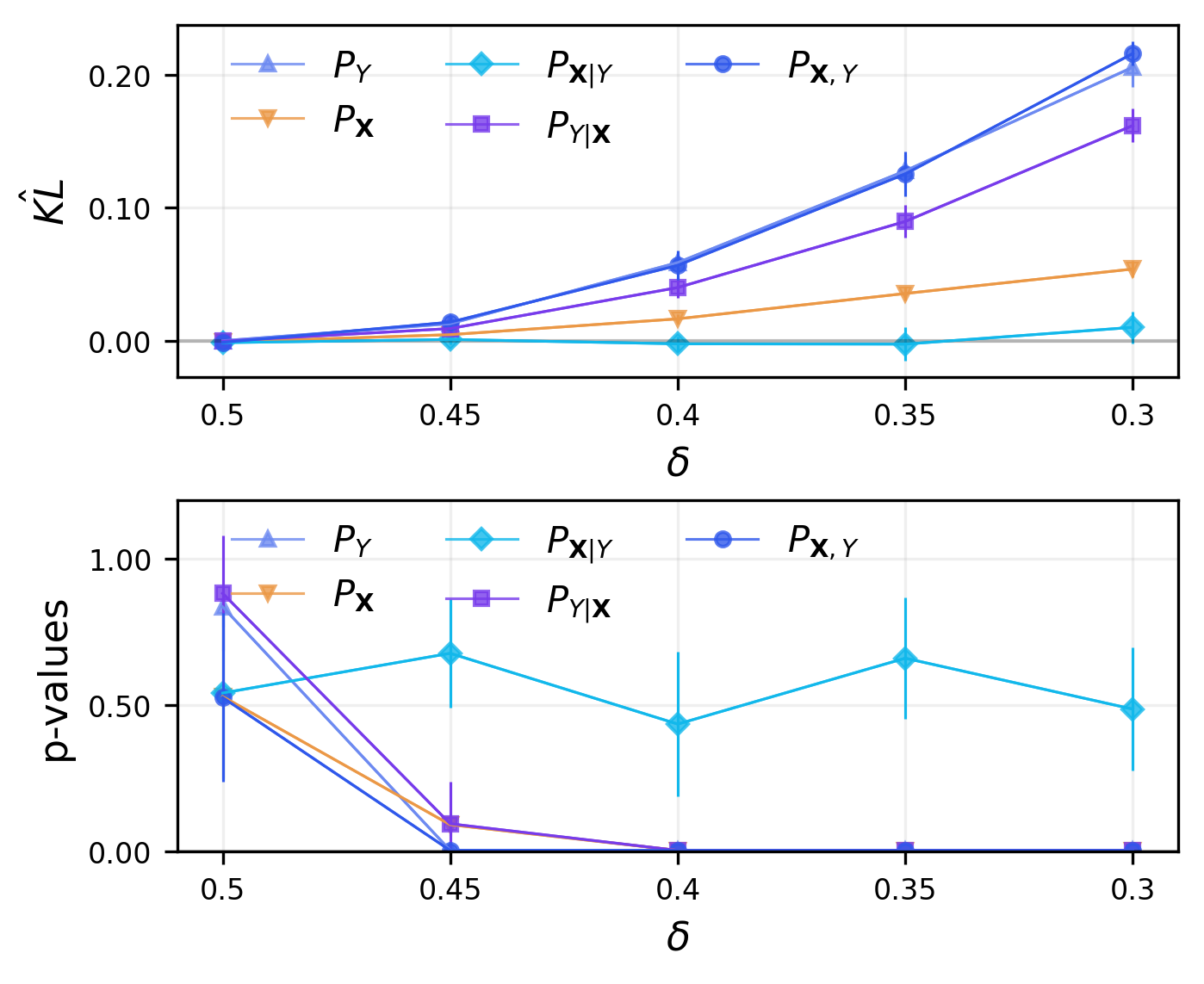
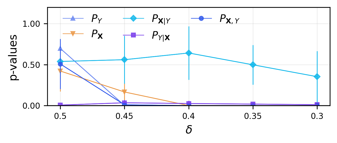
The results are shown in Figure 7, where the lines represent averages across repetitions and error bars give the standard deviations. We were able to detect1414 14 Except when is close to (small or no shift). all types of shift except conditional shift 1 using our approach. This result was expected because, given the class, the distribution of the features must not be affected by how we introduced the shift. We also run results considering the classification-based two-sample test proposed by [25] to test shifts related to joint/marginal distributions and CRT 1 and LPT 1, explained in detail in the appendix, to test for conditional shifts. For the benchmarks, we cannot detect a conditional shift of type 2. A lower power of the benchmarks compared to our method can explain that fact (see artificial data experiments). Furthermore, we cannot compare shift magnitudes using benchmark approaches since their statistics do not have the same nature. We report KL estimates of DetectShift in the appendix. We also left in the appendix an extra (and similar) experiment in which our framework obtained similar p-values compared to the benchmarks.
In summary, we show that our framework can accurately detect the correct shifts even in complex datasets and using deep models.
5 Discussion
The proposed DetectShift framework quantifies and formally tests different dataset shifts, including response, feature, and conditional shifts. Our approach sheds light not only on if a prediction model should be retrained/adapted but also on how, enabling the practitioners to tackle shifts in their data objectively and efficiently. Our method is versatile and applicable across various data types and supervised tasks. Unlike our framework, existing dataset shift detection methods are only designed to detect specific types of shift or cannot formally test their presence, sometimes even requiring both labels and features to be discrete or low-dimensional.
Our experiments have provided compelling evidence of the effectiveness of our framework. Through artificial data experiments, we have demonstrated the versatility of DetectShift in isolating different types of dataset shifts and leveraging supervised learning to construct powerful tests. Furthermore, our framework has shown remarkable performance in higher dimensions, surpassing possible benchmarks. In real data experiments, we have illustrated how DetectShift can extract valuable insights from data, assisting practitioners in adapting their models to changing distributions. Moreover, our approach seamlessly integrates with deep learning models, making it applicable to real-world scenarios. These findings highlight the significant contributions of our framework, showcasing its efficacy in detecting dataset shifts and underscoring its potential for practical applications in various domains.
6 Final remarks and possible extensions
In conclusion, we reflect on key facets and potential limitations inherent to our framework.
Why and how to obtain better Radon-Nikodym derivatives estimates? While Type I error control is not affected by Radon-Nikodym derivatives estimation (as the theoretical results show), the power of the tests is. This happens because the classifiers’ performance in predicting probabilities directly influences how well we approximate the KL divergence and, consequently, can detect shifts in the data. Thus, we can use the cross-entropy (CE) loss on a validation set to pick the best classifier.
Modular framework and alternative statistics choices. Our hypothesis tests are agnostic to the choice test statistics; therefore, our framework is modular. We consider the KL statistics desirable, among other things, because we have the additivity property (Proposition 2), making the analyses more interpretable. A natural alternative to the KL statistics, when we do not want to favor one of the distributions, is the symmetrized KL, for example.
Dealing with streaming data. While the primary design of our framework does not cater to streaming data, it possesses the flexibility for adaptation in such settings. One way of doing this is to group the data into batches (e.g., every hour, day, month) and then apply the proposed approach to compare two or more data batches. Multiple testing methods [35] can be used along with our framework if the practitioner desires.
Labeled data in the target domain. Even though there are many situations in which at least some labeled data are available for the target domain, there are cases in which that is not true. We recognize this scenario as a limitation, warranting further exploration in subsequent research.
7 Acknowledgments
We sincerely thank the “Information Sciences” editor and anonymous reviewers for their invaluable contributions to this paper. We are grateful for their time and dedication in carefully evaluating our manuscript and providing valuable suggestions for improvement.
We are thankful for the credit dataset provided by the Latin American Experian Datalab, the Serasa Experian DataLab. We want to thank the developers of Grammarly and ChatGPT, which were helpful tools when polishing our text.
FMP is grateful for the financial support of CNPq (32857/2019-7) and Fundunesp/Advanced Institute for Artificial Intelligence (AI2) (3061/2019-CCP) during his master’s degree at the University of São Paulo (USP). Part of this work was written when FMP was at USP.
RI is grateful for the financial support of CNPq (309607/2020-5 and 422705/2021-7) and FAPESP (2019/11321-9).
8 Code and data
Our package for dataset shift detection can be found in https://github.com/felipemaiapolo/detectshift
The source code and data used in this paper can be found in https://github.com/felipemaiapolo/dataset_shift_diagnostics.
References
- Abai and Rajmalwar [2019] Zoheb Abai and Nishad Rajmalwar. Densenet models for tiny imagenet classification. arXiv preprint arXiv:1904.10429, 2019.
- Annamoradnejad et al. [2022] Issa Annamoradnejad, Jafar Habibi, and Mohammadamin Fazli. Multi-view approach to suggest moderation actions in community question answering sites. Information Sciences, 600:144–154, 2022. ISSN 0020-0255. doi: https://doi.org/10.1016/j.ins.2022.03.085. URL https://www.sciencedirect.com/science/article/pii/S0020025522003127.
- Bellot and van der Schaar [2019] Alexis Bellot and Mihaela van der Schaar. Conditional independence testing using generative adversarial networks. Advances in Neural Information Processing Systems, 32, 2019.
- Berrett et al. [2020] Thomas B Berrett, Yi Wang, Rina Foygel Barber, and Richard J Samworth. The conditional permutation test for independence while controlling for confounders. Journal of the Royal Statistical Society: Series B (Statistical Methodology), 82(1):175–197, 2020.
- Candès et al. [2018] Emmanuel Candès, Yingying Fan, Lucas Janson, and Jinchi Lv. Panning for gold:‘model-x’knockoffs for high dimensional controlled variable selection. Journal of the Royal Statistical Society: Series B (Statistical Methodology), 80(3):551–577, 2018.
- Conneau et al. [2020] Alexis Conneau, Kartikay Khandelwal, Naman Goyal, Vishrav Chaudhary, Guillaume Wenzek, Francisco Guzmán, Edouard Grave, Myle Ott, Luke Zettlemoyer, and Veselin Stoyanov. Unsupervised cross-lingual representation learning at scale. In ACL, 2020.
- Dalmasso et al. [2021] Niccolo Dalmasso, David Zhao, Rafael Izbicki, and Ann B Lee. Likelihood-free frequentist inference: Bridging classical statistics and machine learning in simulation and uncertainty quantification. arXiv preprint arXiv:2107.03920, 2021.
- Deng et al. [2009] Jia Deng, Wei Dong, Richard Socher, Li-Jia Li, Kai Li, and Li Fei-Fei. Imagenet: A large-scale hierarchical image database. In 2009 IEEE conference on computer vision and pattern recognition, pages 248–255. Ieee, 2009.
- Finlayson et al. [2021] Samuel G Finlayson, Adarsh Subbaswamy, Karandeep Singh, John Bowers, Annabel Kupke, Jonathan Zittrain, Isaac S Kohane, and Suchi Saria. The clinician and dataset shift in artificial intelligence. The New England journal of medicine, 385(3):283, 2021.
- Freeman et al. [2017] Peter E Freeman, Rafael Izbicki, and Ann B Lee. A unified framework for constructing, tuning and assessing photometric redshift density estimates in a selection bias setting. Monthly Notices of the Royal Astronomical Society, 468(4):4556–4565, 2017.
- Gama et al. [2004] Joao Gama, Pedro Medas, Gladys Castillo, and Pedro Rodrigues. Learning with drift detection. In Brazilian symposium on artificial intelligence, pages 286–295. Springer, 2004.
- Ginsberg et al. [2023] Tom Ginsberg, Zhongyuan Liang, and Rahul G Krishnan. A learning based hypothesis test for harmful covariate shift. In The Eleventh International Conference on Learning Representations, 2023. URL https://openreview.net/forum?id=rdfgqiwz7lZ.
- Gretton et al. [2012] Arthur Gretton, Karsten M Borgwardt, Malte J Rasch, Bernhard Schölkopf, and Alexander Smola. A kernel two-sample test. The Journal of Machine Learning Research, 13(1):723–773, 2012.
- Izbicki and Lee [2017] Rafael Izbicki and Ann B Lee. Converting high-dimensional regression to high-dimensional conditional density estimation. Electronic Journal of Statistics, 11(2):2800–2831, 2017.
- Izbicki et al. [2017] Rafael Izbicki, Ann B Lee, and Peter E Freeman. Photo- estimation: An example of nonparametric conditional density estimation under selection bias. The Annals of Applied Statistics, 11(2):698–724, 2017.
- Jang et al. [2022] Sooyong Jang, Sangdon Park, Insup Lee, and Osbert Bastani. Sequential covariate shift detection using classifier two-sample tests. In International Conference on Machine Learning, pages 9845–9880. PMLR, 2022.
- Kim et al. [2021] Ilmun Kim, Matey Neykov, Sivaraman Balakrishnan, and Larry Wasserman. Local permutation tests for conditional independence. arXiv preprint arXiv:2112.11666, 2021.
- Kolmogorov [1933] A N Kolmogorov. Sulla determinazione empirica di una legge di distribuzione. Giorn. Ist. Ital. Attuar., 4:83–91, 1933.
- Krizhevsky et al. [2009] Alex Krizhevsky, Geoffrey Hinton, et al. Learning multiple layers of features from tiny images. 2009.
- Kullback and Leibler [1951] Solomon Kullback and Richard A Leibler. On information and sufficiency. The annals of mathematical statistics, 22(1):79–86, 1951.
- LeCun et al. [1998] Yann LeCun, Léon Bottou, Yoshua Bengio, and Patrick Haffner. Gradient-based learning applied to document recognition. Proceedings of the IEEE, 86(11):2278–2324, 1998.
- Lehmann et al. [2005] Erich Leo Lehmann, Joseph P Romano, and George Casella. Testing statistical hypotheses, volume 3. Springer, 2005.
- Li et al. [2010] Yan Li, Hiroyuki Kambara, Yasuharu Koike, and Masashi Sugiyama. Application of covariate shift adaptation techniques in brain–computer interfaces. IEEE Transactions on Biomedical Engineering, 57(6):1318–1324, 2010.
- Lipton et al. [2018] Zachary Lipton, Yu-Xiang Wang, and Alexander Smola. Detecting and correcting for label shift with black box predictors. In International conference on machine learning, pages 3122–3130. PMLR, 2018.
- Lopez-Paz and Oquab [2016] David Lopez-Paz and Maxime Oquab. Revisiting classifier two-sample tests. arXiv preprint arXiv:1610.06545, 2016.
- Luo et al. [2022] Rachel Luo, Rohan Sinha, Ali Hindy, Shengjia Zhao, Silvio Savarese, Edward Schmerling, and Marco Pavone. Online distribution shift detection via recency prediction. arXiv preprint arXiv:2211.09916, 2022.
- Maia Polo and Vicente [2022] Felipe Maia Polo and Renato Vicente. Effective sample size, dimensionality, and generalization in covariate shift adaptation. Neural Computing and Applications, pages 1–13, 2022.
- Maity et al. [2021] Subha Maity, Diptavo Dutta, Jonathan Terhorst, Yuekai Sun, and Moulinath Banerjee. A linear adjustment based approach to posterior drift in transfer learning. arXiv preprint arXiv:2111.10841, 2021.
- Moreno-Torres et al. [2012] Jose G Moreno-Torres, Troy Raeder, Rocío Alaiz-Rodríguez, Nitesh V Chawla, and Francisco Herrera. A unifying view on dataset shift in classification. Pattern recognition, 45(1):521–530, 2012.
- Pedregosa et al. [2011] Fabian Pedregosa, Gaël Varoquaux, Alexandre Gramfort, Vincent Michel, Bertrand Thirion, Olivier Grisel, Mathieu Blondel, Peter Prettenhofer, Ron Weiss, Vincent Dubourg, et al. Scikit-learn: Machine learning in python. the Journal of machine Learning research, 12:2825–2830, 2011.
- Podkopaev and Ramdas [2021] Aleksandr Podkopaev and Aaditya Ramdas. Tracking the risk of a deployed model and detecting harmful distribution shifts. arXiv preprint arXiv:2110.06177, 2021.
- Polyanskiy and Wu [2022] Yury Polyanskiy and Yihong Wu. Information theory: From coding to learning, 2022.
- Prokhorenkova et al. [2017] Liudmila Prokhorenkova, Gleb Gusev, Aleksandr Vorobev, Anna Veronika Dorogush, and Andrey Gulin. Catboost: unbiased boosting with categorical features. arXiv preprint arXiv:1706.09516, 2017.
- Rabanser et al. [2019] Stephan Rabanser, Stephan Günnemann, and Zachary Lipton. Failing loudly: An empirical study of methods for detecting dataset shift. Advances in Neural Information Processing Systems, 32, 2019.
- Rice et al. [2008] Treva K Rice, Nicholas J Schork, and DC Rao. Methods for handling multiple testing. Advances in genetics, 60:293–308, 2008.
- Saerens et al. [2002] Marco Saerens, Patrice Latinne, and Christine Decaestecker. Adjusting the outputs of a classifier to new a priori probabilities: a simple procedure. Neural computation, 14(1):21–41, 2002.
- Schrouff et al. [2022] Jessica Schrouff, Natalie Harris, Sanmi Koyejo, Ibrahim M Alabdulmohsin, Eva Schnider, Krista Opsahl-Ong, Alexander Brown, Subhrajit Roy, Diana Mincu, Christina Chen, et al. Diagnosing failures of fairness transfer across distribution shift in real-world medical settings. Advances in Neural Information Processing Systems, 35:19304–19318, 2022.
- Simonyan and Zisserman [2014] Karen Simonyan and Andrew Zisserman. Very deep convolutional networks for large-scale image recognition. arXiv preprint arXiv:1409.1556, 2014.
- Smirnov [1939] Nikolai V Smirnov. Estimate of deviation between empirical distribution functions in two independent samples. Bulletin Moscow University, 2(2):3–16, 1939.
- Sønderby et al. [2016] Casper Kaae Sønderby, Jose Caballero, Lucas Theis, Wenzhe Shi, and Ferenc Huszár. Amortised map inference for image super-resolution. arXiv preprint arXiv:1610.04490, 2016.
- Speakman et al. [2018] Skyler Speakman, Srihari Sridharan, and Isaac Markus. Three population covariate shift for mobile phone-based credit scoring. In Proceedings of the 1st ACM SIGCAS Conference on Computing and Sustainable Societies, pages 1–7, 2018.
- Sugiyama and Kawanabe [2012] Masashi Sugiyama and Motoaki Kawanabe. Machine learning in non-stationary environments: Introduction to covariate shift adaptation. MIT press, 2012.
- Sugiyama et al. [2007] Masashi Sugiyama, Matthias Krauledat, and Klaus-Robert Müller. Covariate shift adaptation by importance weighted cross validation. Journal of Machine Learning Research, 8(5), 2007.
- Sugiyama et al. [2012] Masashi Sugiyama, Taiji Suzuki, and Takafumi Kanamori. Density ratio estimation in machine learning. Cambridge University Press, 2012.
- Vaz et al. [2019] Afonso Fernandes Vaz, Rafael Izbicki, and Rafael Bassi Stern. Quantification under prior probability shift: The ratio estimator and its extensions. The Journal of Machine Learning Research, 20(1):2921–2953, 2019.
- Vovk [2020] Vladimir Vovk. Testing for concept shift online. arXiv preprint arXiv:2012.14246, 2020.
- Webb et al. [2018] Geoffrey I Webb, Loong Kuan Lee, Bart Goethals, and François Petitjean. Analyzing concept drift and shift from sample data. Data Mining and Knowledge Discovery, 32(5):1179–1199, 2018.
- Wijaya et al. [2021] Maleakhi A Wijaya, Dmitry Kazhdan, Botty Dimanov, and Mateja Jamnik. Failing conceptually: Concept-based explanations of dataset shift. arXiv preprint arXiv:2104.08952, 2021.
- Xu and Klabjan [2021] Yiming Xu and Diego Klabjan. Concept drift and covariate shift detection ensemble with lagged labels. In 2021 IEEE International Conference on Big Data (Big Data), pages 1504–1513. IEEE, 2021.
- Yu et al. [2019] Shujian Yu, Zubin Abraham, Heng Wang, Mohak Shah, Yantao Wei, and José C Príncipe. Concept drift detection and adaptation with hierarchical hypothesis testing. Journal of the Franklin Institute, 356(5):3187–3215, 2019.
Appendix A Methodology
A.1 Alternative estimator for when is discrete
Assume is the range of in the target domain, where is finite. Define , for . Then, we can write . Having observed two datasets (in practice, we use the test datasets), and , we define to be the relative frequency of the label in dataset . Then, a plug-in estimator for is given by . This estimator is consistent.
A.2 Algorithm to obtain -values
In practice, can be a very small number, e.g., .
A.3 Proofs
The results presented in this section are not original; however, we decided to include proofs to make this work self-contained.
Proof.
In this proof, we assume the distributions are absolutely continuous with respect to the Lebesgue measure. For a more general proof, see Polyanskiy and Wu 2022 (Theorem 2.13).
We start showing . Let and be the joint densities of and with respect to the Lebesgue measure. Then
We can show that analogously. ∎
Proposition 3. Let be a -value obtained from Algorithm 1 (appendix) with fixed and . Then, for every ,
- •
Under ,, and (if is discrete),
- •
Under
where is the total variation distance, , , and .
Proof.
We start deriving the result for using the theory behind permutation tests for two-sample/independence tests (see Lehmann et al. 2005 for more details). The results for and obtained analogously. Define and , for all , where ’s are i.i.d. . For the rest of the proof, ’s will always be noisy versions of the respective ’s.
Recall that
See that gives the rank of among all ’s, that is, if it means that there are values of such that . If and the permutations are drawn uniformly from the set of all permutations of , then are exchangeable. Because we add ’s in ’s, we can guarantee that all ’s are different with probability 1. Consequently, is uniformly distributed in . Then,
where is the floor function.
The result for is obtained similarly. Assume that for every . We can ignore values of not in because does not depend on them. Given that we permute samples within each level of , we have that are exchangeable, implying that (by our derivations above)
The result for is based on Theorem 4 of Berrett et al. 2020. For each , denote where , for each from elements of . Define and let be one extra dataset built in the same way as all others considering . See that all datasets considering share the same values for the covariates; let denote a random matrix containing such values for all samples. Because the p-values only depend on the data coming from1515 15 If that was not true, the following inequality would hold if we condition not only on but also on a matrix composed of ’s (as done in Berrett et al. 2020). (and not on the full test set ), we have that
where is the p-value calculated using instead of . This step is justified by the definition of the total variation distance and by a conditional independence argument [4] (given , all data replications are conditionally independent).
By construction, are exchangeable given , we have that . Then, taking expectations on both sides of the inequality above, we get
∎
Realize that the last result is true even if does not hold. However, if is not true, we do not expect to be small.
Appendix B Experiments
B.1 Comparisons with existing approaches (more details)
Some details about the experiments were omitted from the main text: (i) how we choose when testing for conditional shift 2; (ii) how the local permutation tests (LPT) and conditional randomization tests (CRT) alternatives work and what statistic they use.
B.1.1 How do we choose in this set of experiments?
Given that our main objective in this experiment is comparing the power of different tests that use the same approximated distribution , we choose to fix , where is the conditional distribution of under .
B.1.2 How do the LPT and CRT alternative tests work, and what statistics do they use?
We start explaining the two CRT alternative tests, which work in the same way but have different test statistics.
- 1.
We split our dataset in a training set and a test set ;
- 2.
We build an artificial training set , where are sampled from ;
- 3.
We train a probabilistic classifier to distinguish samples from and , where the original set receives label 1 and the artificial data receives label 0;
- 4.
For , we test each of the hypotheses of interest by computing a -value of the form
where is a test statistic depending on and each is obtained sampling different labels from . When
we have CRT 1. When
we have CRT 2.
The LPT alternative tests work in the same way. The only difference is that the "artificial" variables are obtained via local permutation within levels.
represents a CatBoost classifier in this experiment. When is a logistic regressor (like in the KL tests), at least one test is too conservative.
B.2 Digits experiment
MNIST samples tend to have more white pixels than USPS (Figure 8); thus, the distributions of are different in both datasets.
 |
 |
B.3 A regression experiment
We present a regression experiment using data from 2017, 2018, 2019, and 2020 of ENEM1616 16 Data extracted from https://www.gov.br/inep/pt-br/acesso-a-informacao/dados-abertos/microdados/enem, the “Brazilian SAT.” In each of the years, is given by the students’ math score in a logarithmic scale while is composed of six of their personal and socioeconomic features: gender, race, school type (private or public), mother’s education, family income and the presence of a computer at home. We randomly subsample the data in each one of the years to 30k data points with of them going to the test portion and then use the CatBoost algorithm to estimate the Radon-Nikodym derivative and the conditional distribution of . When estimating the distribution of , we first fit a regressor to predict given , and then, using a holdout set, we fit a Gaussian model on the residuals. When testing for a shift in the distribution, we discretize in 10 bins, evenly splitting the data. Even though we use the binned version of to get the -value, we report in the first panel of Figure 9. In this experiment, we do a similar analysis compared to the credit one, comparing the probability distributions of 2018, 2019, and 2020 with the one in 2017. From Figure 9, it is possible to see that we detected all kinds of shifts after 2017. This result indicates that a model trained in 2017 might not generalize well to other years, and practitioners may consider retraining their models from scratch using more recent data.

B.4 Detecting shifts with deep models
B.4.1 Extra plot

B.4.2 Extra results
We include one extra experiment using the ‘‘60k Stack Overflow Questions with Quality Rating" dataset1717 17 https://www.kaggle.com/datasets/imoore/60k-stack-overflow-questions-with-quality-rate [2]. This dataset has three classes of rating from Stack Overflow questions. We repeat the same procedure to obtain results for the other deep-learning experiments.
| Ours |
 |
| Benchmark |
 |
B.5 Experiments running time
All the experiments were run in a MacBook Air (M1, 2020) 16GB, except for the credit analysis experiment in an 80 CPUs Intel Xeon Gold 6148 cluster. We consider one iteration as all the steps needed to compute all the -values used for a specific experiment. In the artificial data experiments, on average, each iteration performed by our framework took less than , while in real data experiments, each iteration took less than .