Centroidal Aerodynamic Modeling and Control
of Flying Multibody Robots

• •

  $\mathcal{I}=\{O;\boldsymbol{X},\boldsymbol{Y},\boldsymbol{Z}\}$ denotes an inertial frame, composed of a point (origin) and an orientation w.r.t. which the vehicle’s absolute pose is measured.

• •

  $\mathcal{B}$ denotes the base frame, i.e. a frame rigidly attached to the robot base link;

• •

  $\mathcal{G}[\mathcal{I}]$ is a frame with the origin at the robot center of mass and the same orientation of the inertial frame;

• •

  ${}^{\mathcal{I}}o_{\mathcal{G}}\in\mathbb{R}^{3}$ is the center of mass (CoM) position of the robot expressed in the inertial frame. ${}^{\mathcal{I}}\boldsymbol{v}_{CoM}\in\mathbb{R}^{3}$ denotes the linear velocity of the robot CoM w.r.t. the inertial frame origin expressed in the inertial frame;

• •

  ${}^{\mathcal{I}}\boldsymbol{v}_{a}\in\mathbb{R}^{3}$ indicates the relative velocity between the wind and the robot CoM expressed in the inertial frame, i.e. ${}^{\mathcal{I}}\boldsymbol{v}_{a}={}^{\mathcal{I}}\boldsymbol{v}_{CoM}-{}^{\mathcal{I}}\boldsymbol{v}_{w}$, with ${}^{\mathcal{I}}\boldsymbol{v}_{w}\in\mathbb{R}^{3}$ the absolute wind velocity¹¹ 1 In the remainder of the paper, we omit the superscript $\mathcal{I}$ unless it is necessary to explicitly write it for the sake of clarity, and we write ${}^{\mathcal{I}}\boldsymbol{v}_{a}=\boldsymbol{v}_{a}$.;

• •

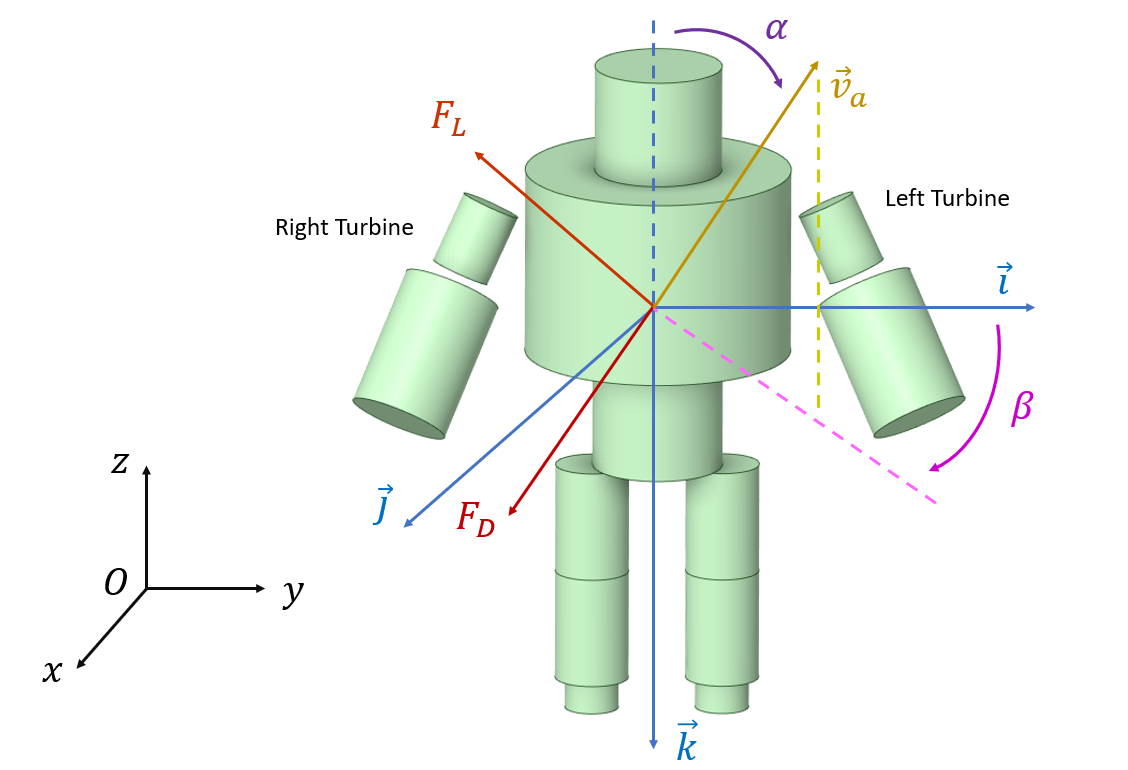
  $\mathcal{D}=\{{}^{\mathcal{I}}o_{\mathcal{G}};\boldsymbol{i},\boldsymbol{j},\boldsymbol{k}\}$ represents the body frame. The $\boldsymbol{k}$ axis direction is parallel to the chest cylinder principal axis, pointing towards the legs. The $\boldsymbol{i}$ axis is normal to the robot symmetry plane, pointing towards left arm. The $\boldsymbol{j}$ axis is defined by the right-hand rule.

The flying humanoid robot is modeled as a multi-body, floating-base system composed of $n+1$ rigid bodies (links). Each body is connected to the others by means of 1-DoF joints, for a total of $n$ DoF. The set of robot configurations belongs to a space defined as: $\mathbb{Q}\in\mathbb{R}^{3}\times SO(3)\times\mathbb{R}^{n}$. The triplet $q=({}^{\mathcal{I}}o_{\mathcal{B}},{}^{\mathcal{I}}R_{\mathcal{B}},s)\in\mathbb{Q}$ is composed by $({}^{\mathcal{I}}o_{\mathcal{B}},{}^{\mathcal{I}}R_{\mathcal{B}})$, which represent the position and orientation of the base frame $\mathcal{B}$ w.r.t. the inertial frame, and by the robot internal shape $s\in\mathbb{R}^{n}$ represented by the joints angles. The system velocities belong to the space $\mathbb{V}\in\mathbb{R}^{3}\times\mathbb{R}^{3}\times\mathbb{R}^{n}$. An element of $\mathbb{V}$ is given by $v=(\nu_{\mathcal{B}},\dot{s})$ where $\nu_{\mathcal{B}}=({}^{\mathcal{I}}v_{\mathcal{B}},{}^{\mathcal{I}}\omega_{\mathcal{B}})$ is the linear and angular velocity of the base frame w.r.t. the inertial frame, while $\dot{s}$ are the joints velocities.

The floating-base system equations of motions can be derived following the Euler-Poincar$\acute{e}$ formalism [18]:

where $M$, $C\in\mathbb{R}^{n+6\times n+6}$ are the mass and Coriolis matrices, $G\in\mathbb{R}^{n+6}$ is the gravity vector, $\tau\in\mathbb{R}^{n}$ are the internal actuation torques and $F_{k}$ is the $k^{th}$ external force acting on the system. In the case under study, we assume that the forces acting on the robot during flight are the aerodynamic forces and the thrust forces generated by the jet-engines. Here, we consider in the model only the thrust generated by the jet-engines, while how to add the aerodynamic forces in Eq. (1) will be treated later on in the paper. Hence, each $F_{k}\in\mathbb{R}^{3}$ represents the thrust force applied on the robot by the $k^{th}$ jet, and we rewrite $F_{k}={}^{\mathcal{I}}l_{k}T_{k}$, where ${}^{\mathcal{I}}l_{k}\in\mathbb{R}^{3}$ is the direction of thrust force, while $T_{k}\in\mathbb{R}$ is the thrust intensity. The jacobian $J_{k}(q)$ is the map between the system velocity $v$ and the linear velocity ${}^{\mathcal{I}}v_{k}$ of the $k^{th}$ thrust application point. We can then define the thrusts vector $T\mathrel{\mathop{\mathchar 58\relax}}=(T_{1},T_{2},T_{3},T_{4})^{\top}$ and rewrite $\sum^{n_{c}}_{k=1}J_{k}^{\top}F_{k}=f(q,T)$.

We introduce ${}^{\mathcal{G}[\mathcal{I}]}\boldsymbol{h}\in\mathbb{R}^{6}$ to denote the robot total momentum expressed w.r.t. ^G[I], namely:

where ${}^{\mathcal{G}[\mathcal{I}]}\boldsymbol{h}^{p}\in\mathbb{R}^{3}$ and ${}^{\mathcal{G}[\mathcal{I}]}\boldsymbol{h}^{\omega}\in\mathbb{R}^{3}$ are the linear and angular momentum, respectively. In addition, the following holds: ${}^{\mathcal{I}}\boldsymbol{v}_{CoM}=\frac{1}{m}{}{{}^{\mathcal{G}[\mathcal{I}]}}\boldsymbol{h}^{p}.$ The robot total momentum corresponds to the summation of all the links momenta ${}_{B}\boldsymbol{h}^{i}$, measured in the base frame and projected on ${\mathcal{G}[\mathcal{I}]}$: ${}^{\mathcal{G}[\mathcal{I}]}\boldsymbol{h}=\sum_{i}{}_{{}^{\mathcal{G}[\mathcal{I}]}}\boldsymbol{X}^{B}{}_{B}\boldsymbol{h}^{i},$ with ${}_{{}^{\mathcal{G}[\mathcal{I}]}}\boldsymbol{X}^{B}\in\mathbb{R}^{6\times 6}$ the adjoint matrix transforming a wrench expressed in $B$ into one expressed in ${\mathcal{G}[\mathcal{I}]}$. Then:

with $\boldsymbol{I}_{i}\in\mathbb{R}^{6\times 6}$ being the (constant) link inertia expressed in link frame. Hence, one obtains: ${}^{\mathcal{G}[\mathcal{I}]}\boldsymbol{h}=\boldsymbol{J}_{\text{CMM}}\boldsymbol{v},$ where $\boldsymbol{J}_{\text{CMM}}\in\mathbb{R}^{6\times n}$ is the Centroidal Momentum Matrix (CMM) [4]. The rate of change of the centroidal momentum balances the external wrenches applied to the robot, i.e.:

where ${}_{{}^{\mathcal{G}[\mathcal{I}]}}\boldsymbol{X}^{k}\in\mathbb{R}^{6\times 6}$ is the adjoint matrix that transforms an external wrench from the application frame (located in ${}^{\mathcal{I}}o_{k}$ with orientation ${}^{\mathcal{I}}R_{k}$) to ${\mathcal{G}[\mathcal{I}]}$. Finally, $\bar{\boldsymbol{g}}$ is the 6D gravity acceleration vector.

In the sequel, we consider the overall aerodynamic effects that can be described as an external force $\boldsymbol{F_{a}}\in\mathbb{R}^{3}$ applied at the robot center of mass, thus acting on both (4) and (1).

Considering Assumption 1, CFD simulations are all performed with fixed robot initial joint positions, which is supposed to been optimized given a flight metric (e.g. minimisation of thrust forces). Furthermore, a complex-shaped geometry as the iRonCub one can cause difficulties in the meshing phase of CFD simulations, because of errors caused by interference among complex parts. Therefore, we approximate the geometry of iRonCub representing the major robot links as simple cylinders (see Fig. 2). The model allows to obtain high-quality meshes with a relatively low number of elements, which in turn translates in a reduction of the simulation time.

For the sole purpose of CFD analysis, let us introduce the frame $\mathcal{A}=\{{}^{\mathcal{I}}o_{\mathcal{G}};\boldsymbol{i}_{a},\boldsymbol{j}_{a},\boldsymbol{k}_{a}\}$ as the relative velocity frame. It is defined for CFD simulations only, where the relative velocity is always different from zero, namely $|\boldsymbol{v}_{a}|\neq 0$. The $\boldsymbol{j}_{a}$ axis therefore aligns to the opposite direction of $\boldsymbol{v}_{a}$ (see also Fig. 3).

Significant robot flight configurations, corresponding to precise values of $\alpha$ and $\beta$, were simulated using CFD tools. In total 45 simulations were run, with $\alpha\in($$,\ $$,\ $$,\ $$,\ $$,\ $$,\ $$,\ $$,\ $$)$ and $\beta\in($$,\ $$,\ $$,\ $$,\ $$)$ which supplied the necessary data for proceeding with the modeling of aerodynamic characteristics on iRonCub. Settings of CFD simulations are schematically reported in Table I.

As introduced in Sec. III-B, the three dimensionless functions $C_{D}$, $C_{S}$, $C_{N}$ are the aerodynamic characteristics of the body, i.e. the defined aerodynamic coefficients (AC): drag coefficient, sideforce coefficient and normal force coefficient. In this section, the analytical model of AC is identified based on the CFD results from Sec. III-B. To proceed with identification, the following assumptions are made:

1. 1.

   the aerodynamic forces act at the robot’s CoM (coincides with CoP) and therefore the aerodynamic moments ${M}_{a}$ are equal to zero;

2. 2.

   from CFD results, the sideforce effect is neglected due to its small magnitude compared with the other two aerodynamic force components, and with other forces acting on the robot;

3. 3.

   the AC dependence from Mach number $\mathcal{M}$ is considered negligible since the relative velocity intensity of the robot is much smaller than the sound speed (i.e. the density can be assumed as constant);

4. 4.

   the AC dependence from Reynolds number $Re$ is not considered since the AC evaluated from CFD for different values of relative velocity doesn’t show a significant dependence from it;

5. 5.

   the effects of rotational and unsteady motions of the vehicle on its surrounding airflow are negligible [19].

As a consequence, the AC depend only on the flight configuration $(\alpha,\beta)$ and can be written as [16]:

Considering that the aerodynamic coefficients are naturally $2\pi$-periodic [23], $\sin{(\cdot)}$ functions are used to design the mathematical models of AC:

As previously mentioned, the zero sideforce assumption allows the identification of the lift force with the normal force, as demonstrated in [16] for axisymmetric bodies, since the normal component of the aerodynamic force lies on the $\boldsymbol{v}_{a}-\boldsymbol{k}_{a}$ plane. The aerodynamic forces acting on the robot CoM rewrite as:

where $\boldsymbol{r}(\beta)=-\sin(\beta)\boldsymbol{i}+\cos(\beta)\boldsymbol{j}.$

The iRonCub flight controller [14, 15] is a task-based control strategy, composed of several control objectives (tasks), with different priorities. The so-called primary task, i.e. the task with the higher priority, is the stabilization of the robot’s centroidal momentum²² 2 The centroidal momentum is the robot total momentum expressed w.r.t. the frame $\mathcal{G}[\mathcal{I}]$ defined in Sec. II. dynamics, which equals the summation of all external forces acting on the robot:

where $m$ is the robot’s total mass, $\boldsymbol{A}(q)\in\mathbb{R}^{6\times m}$ is a proper matrix mapping the thrust vector $T$ in the momentum equation. For the momentum control design, we assume that the robot joints velocities $\dot{s}$ and the thrust rate of change $\dot{T}$ can be chosen at will, and then can be considered as our control inputs. Therefore, we define $u\mathrel{\mathop{\mathchar 58\relax}}=(\dot{T},\dot{s})$. To make the control input $u$ appear in the momentum equation (10), we increase the relative degree of the output and write the momentum acceleration:

As demonstrated in our previous works [14, 15], it is possible to find a smooth control input $u^{*}$ that renders the closed-loop equilibrium point $(\dot{\tilde{\boldsymbol{h}}},\tilde{\boldsymbol{h}},\boldsymbol{I})=(\boldsymbol{0},\boldsymbol{0},\boldsymbol{0})$ globally asymptotically stable, where $\tilde{\boldsymbol{h}}=\boldsymbol{h}-\boldsymbol{h}^{d}$, $\boldsymbol{h}^{d}$ is the reference momentum trajectory and $\boldsymbol{I}\mathrel{\mathop{\mathchar 58\relax}}=\int_{0}^{t}\tilde{\boldsymbol{h}}$.

We also define a postural task to resolve the redundancy in the control input $u$ and maintain the robot configuration close to a desired shape:

with $s^{d}$ the desired robot posture and $K_{P}^{s}\in\mathbb{R}^{n\times n}$ a positive gains matrix. The two tasks are then achieved by means of Quadratic Programming (QP) optimization framework:

where soft task priorities are assigned to the two tasks via proper weights $w_{1},w_{2}>0$. Framing the problem as an optimization procedure allows to include input boundaries $u_{min},u_{max}$ in the control design. It is also possible to include the integral of input boundaries (namely, the joint position and thrust limits) in the QP design. For more details on these aspects of the flight control design, which are not relevant for this paper, we refer to previous works [14, 15].

The flight controller discussed in IV-A does not consider the effect of aerodynamic forces. This missing information may impair the performances of the control algorithm when aerodynamic forces are not negligible. To overcome this limitation, we implemented two modifications of the iRonCub flight controller: feedback linearization and gain scheduling. To implement our control strategy, we considered the following Assumption 2: we assume that $\dot{\boldsymbol{F}}_{a}=0$ in the calculation of the momentum acceleration.

The robot dynamics is simulated by numerically integrating the equations of motion with aerodynamic forces Eq. (14) in a custom-made simulator implemented in MATLAB-Simulink. The controller is entirely designed in Simulink and runs at a frequency of $100\text{\,}\mathrm{H}\mathrm{z}$. A fast, inner torque control loop is designed to stabilize the joints velocities $\dot{s}$ towards the reference values generated with Eq. (13).

We designed a flight envelope composed as follows:

1. 1.

   Scenario 1: the robot hovers in vertical position, while subject to a wind in the frontal direction that follows the profile depicted in Fig. 5.

2. 2.

   Scenario 2: the robot hovers and climbs to gain altitude, then moves forward at around $11\text{\,}\mathrm{m}\mathrm{/}\mathrm{s}$, in presence of a lateral wind with the profile of Fig. 6.

The wind profiles are composed of a constant wind of $3\text{\,}\mathrm{m}\mathrm{/}\mathrm{s}$, and wind gusts of different shapes with magnitude of $10\text{\,}\mathrm{m}\mathrm{/}\mathrm{s}$ and $15\text{\,}\mathrm{m}\mathrm{/}\mathrm{s}$ [39, 40, 41].

We evaluate the performances of three control strategies: the baseline controller of [14][15], the feedback linearization control designed in Sec. IV, and a third controller that uses gain scheduling as described in Sec. IV. To test the robustness of feedback linearization controller, the aerodynamic force $F_{a}$ in the control model is computed assuming random noise of $5\text{\,}\%$ and a calibration error of $10\text{\,}\%$ on both $\alpha$ and $\beta$ angles.

Simulation results for the hovering scenario are presented in Fig. 5, where we focused on the linear and angular momentum error norm and center of mass position error. With baseline controller, the center of mass error along the wind direction has peaks of $50\text{\,}\mathrm{c}\mathrm{m}$ and $35\text{\,}\mathrm{c}\mathrm{m}$ in correspondence of the wind gusts (shaded area), which are reduced by $33\text{\,}\%$ when the gain scheduling control is used and by $71\text{\,}\%$ for the feedback linearization control. The linear momentum error also reduces accordingly, while the angular momentum error remains comparable in all three simulations.

The three controllers are then tested during high speed flight. Fig. 6 compare their performances in this second scenario: the baseline controller has the worst performances, with peaks errors on the center of mass position of $75\text{\,}\mathrm{c}\mathrm{m}$ and $50\text{\,}\mathrm{c}\mathrm{m}$. The gain scheduling controller is able to reduce the center of mass peaks error by $30\text{\,}\%$, while the feedback linearization further reduces the peaks by $95\text{\,}\%$. Linear and angular momentum errors also behave in accordance with the results already achieved for Scenario 1.

References

- [1] A. E. Jimenez-Cano et al., ”Control of an aerial robot with multi-link arm for assembly tasks,” 2013 IEEE International Conference on Robotics and Automation, 2013, pp. 4916-4921, doi: 10.1109/ICRA.2013.6631279.
- [2] G. Heredia et al., ”Control of a multirotor outdoor aerial manipulator,” 2014 IEEE/RSJ International Conference on Intelligent Robots and Systems, 2014, pp. 3417-3422, doi: 10.1109/IROS.2014.6943038.
- [3] D. Mellinger et al., ”Design, modeling, estimation and control for aerial grasping and manipulation,” 2011 IEEE/RSJ International Conference on Intelligent Robots and Systems, 2011, pp. 2668-2673, doi: 10.1109/IROS.2011.6094871.
- [4] David E. Orin and Ambarish Goswami, ”Centroidal Momentum Matrix of a humanoid robot: Structure and properties”, Intelligent Robots and Systems, 2008. IROS 2008. IEEE/RSJ International Conference on, 2008, pp. 653 - 659.
- [5] A. Ollero et al., ”Past, Present, and Future of Aerial Robotic Manipulators,” in IEEE Transactions on Robotics, doi: 10.1109/TRO.2021.3084395.
- [6] Qian Wang and R. F. Stengel, ”Robust nonlinear flight control of a high-performance aircraft,” in IEEE Transactions on Control Systems Technology, vol. 13, no. 1, pp. 15-26, Jan. 2005, doi: 10.1109/TCST.2004.833651.
- [7] M. Pitonyak and F. Sahin, ”A novel hexapod robot design with flight capability,” 2017 12th System of Systems Engineering Conference (SoSE), 2017, pp. 1-6, doi: 10.1109/SYSOSE.2017.7994965.
- [8] A. Kalantari and M. Spenko, ”Design and experimental validation of HyTAQ, a Hybrid Terrestrial and Aerial Quadrotor,” 2013 IEEE International Conference on Robotics and Automation, 2013, pp. 4445-4450, doi: 10.1109/ICRA.2013.6631208.
- [9] Mohamed H. A. Omer et al., ”Momentum-Based Extended Kalman Filter for Thrust Estimation on Flying Multibody Robots” 2022 IEEE Robotics and Automation Letters, pp. 526-533, doi: 10.1109/LRA.2021.3129258.
- [10] A. Bozkurt, A. Lal and R. Gilmour, ”Aerial and terrestrial locomotion control of lift assisted insect biobots,” 2009 Annual International Conference of the IEEE Engineering in Medicine and Biology Society, 2009, pp. 2058-2061, doi: 10.1109/IEMBS.2009.5334433.
- [11] ”Caltech Building Agile Humanoid Robot by Combining Legs With Thrusters”, 2019, https://spectrum.ieee.org/caltech-building-agile-humanoid-robot-by-combining-legs-with-thrusters.
- [12] Z. Huang et al., ”Jet-HR1: Two-dimensional bipedal robot step over large obstacle based on a ducted-fan propulsion system,” 2017 IEEE-RAS 17th International Conference on Humanoid Robotics (Humanoids), 2017, pp. 406-411, doi: 10.1109/HUMANOIDS.2017.8246905.
- [13] Natale, Lorenzo et al., ”iCub: The not-yet-finished story of building a robot child”, Science Robotics vol. 2, no. 13, 2017, doi: 10.1126/scirobotics.aaq1026, https://robotics.sciencemag.org/content/2/13/eaaq1026.
- [14] D. Pucci, S. Traversaro and F. Nori, ”Momentum Control of an Underactuated Flying Humanoid Robot,” in IEEE Robotics and Automation Letters, vol. 3, no. 1, pp. 195-202, Jan. 2018, doi: 10.1109/LRA.2017.2734245.
- [15] G. Nava et al., ”Position and Attitude Control of an Underactuated Flying Humanoid Robot,” 2018 IEEE-RAS 18th International Conference on Humanoid Robots (Humanoids), 2018, pp. 1-9, doi: 10.1109/HUMANOIDS.2018.8624985.
- [16] D. Pucci et al., Nonlinear feedback control of axisymmetric aerial vehicles. Automatica 53 (2015) 72-78
- [17] G. L’Erario et al., ”Modeling, Identification and Control of Model Jet Engines for Jet Powered Robotics,” in IEEE Robotics and Automation Letters, vol. 5, no. 2, pp. 2070-2077, April 2020, doi: 10.1109/LRA.2020.2970572.
- [18] J. E. Marsden and T. S. Ratiu, Introduction to Mechanics and Symmetry: A Basic Exposition of Classical Mechanical Systems. Springer Publishing Company, Incorporated, 2010.
- [19] Stengel, Robert F. Flight Dynamics: , Princeton: Princeton University Press, 2015.
- [20] F. Ruggiero, V. Lippiello and A. Ollero, ”Aerial Manipulation: A Literature Review,” in IEEE Robotics and Automation Letters, vol. 3, no. 3, pp. 1957-1964, July 2018, doi: 10.1109/LRA.2018.2808541.
- [21] H. Huang et al., ”Aerodynamics and control of autonomous quadrotor helicopters in aggressive maneuvering,” 2009 IEEE International Conference on Robotics and Automation, 2009, pp. 3277-3282, doi: 10.1109/ROBOT.2009.5152561.
- [22] M. Orsag et al., ”Dexterous Aerial Robots—Mobile Manipulation Using Unmanned Aerial Systems,” in IEEE Transactions on Robotics, vol. 33, no. 6, pp. 1453-1466, Dec. 2017, doi: 10.1109/TRO.2017.2750693.
- [23] Z. V. Didyk and V. A. Apostolyuk, ”Whole angle approximations of aerodynamic coefficients,” 2012 2nd International Conference ”Methods and Systems of Navigation and Motion Control” (MSNMC), 2012, pp. 119-121, doi: 10.1109/MSNMC.2012.6475107.
- [24] A. Roberts and A. Tayebi, ”Adaptive Position Tracking of VTOL UAVs,” in IEEE Transactions on Robotics, vol. 27, no. 1, pp. 129-142, Feb. 2011, doi: 10.1109/TRO.2010.2092870.
- [25] G. Antonelli et al., ”Adaptive trajectory tracking for quadrotor MAVs in presence of parameter uncertainties and external disturbances,” 2013 IEEE/ASME International Conference on Advanced Intelligent Mechatronics, 2013, pp. 1337-1342, doi: 10.1109/AIM.2013.6584280.
- [26] D. Cabecinhas, R. Cunha and C. Silvestre, ”A nonlinear quadrotor trajectory tracking controller with disturbance rejection,” 2014 American Control Conference, 2014, pp. 560-565, doi: 10.1109/ACC.2014.6858615.
- [27] F. Ruggiero et al., ”Impedance control of VToL UAVs with a momentum-based external generalized forces estimator,” 2014 IEEE International Conference on Robotics and Automation (ICRA), 2014, pp. 2093-2099, doi: 10.1109/ICRA.2014.6907146.
- [28] M. Hua et al., ”Introduction to feedback control of underactuated VTOLvehicles: A review of basic control design ideas and principles,” in IEEE Control Systems Magazine, vol. 33, no. 1, pp. 61-75, Feb. 2013, doi: 10.1109/MCS.2012.2225931.
- [29] A. Mokhtari and A. Benallegue, ”Dynamic feedback controller of Euler angles and wind parameters estimation for a quadrotor unmanned aerial vehicle,” IEEE International Conference on Robotics and Automation, 2004. Proceedings. ICRA ’04. 2004, 2004, pp. 2359-2366 Vol.3, doi: 10.1109/ROBOT.2004.1307414.
- [30] I. Kroo et al., “The mesicopter: A miniature rotorcraft concept, phase ii interim report,” 2000.
- [31] Daniele Pucci. ”Towards a unified approach for the control of aerial vehicles”. Other. Université Nice Sophia Antipolis, 2013. English. ffNNT : 2013NICE4022ff. fftel-00865829f
- [32] Cook, M. V. (2012). ”Flight dynamics principles: a linear systems approach to aircraft stability and control”. Butterworth-Heinemann.
- [33] de Divitiis, N. and Vitale, A. (2010). ”Fully structured aerodynamic model for parameter identification of a re-entry experimental vehicle”. Journal of Spacecraft and Rockets, 47:113–124.
- [34] Fujimori, A. and Ljung, L. (2006). ”Model identification of linear parameter varying aircraft systems”. Proceedings of the Institution of Mechanical Engineers, Part G: Journal of Aerospace Engineering, 220(4):337–346.
- [35] Albisser, M. et al. (2013). ”Identifiability investigation of the aerodynamic coefficients from free flight tests”. In AIAA Atmospheric Flight Mechanics Conference, Boston, Massachusetts.
- [36] Buresti, G.. ”Bluff-body aerodynamics” lecture notes, Wind-excited and aeroelastic vibrations of structures. Department of Aerospace Engineering, University of Pisa, Italy.
- [37] D. Pucci et al., “Towards Aerial Humanoid Robotics Unifying Robotic Platforms for Manipulation, Aerial, and Terrestrial Locomotion”. [Online].
- [38] Nori, F. et al. (2015). iCub whole-body control through force regulation on rigid non-coplanar contacts. Frontiers in Robotics and AI, 2, 6.
- [39] Ghoreyshi, Mehdi et al. (2018). Simulation and Modeling of Rigid Aircraft Aerodynamic Responses to Arbitrary Gust Distributions, Aerospace, 2, 5.
- [40] J. Gu et al., ”Design of the Wind Turbine Simulation System Based on Fuzzy Control,” 2019 6th International Conference on Systems and Informatics (ICSAI), 2019, pp. 268-273, doi: 10.1109/ICSAI48974.2019.9010187.
- [41] J.-M. Kai and T. Hamel and C. Samson, ”A unified approach to fixed-wing aircraft path following guidance and control,” Automatica, 2019, pp. 108491, doi: 10.1016/j.automatica.2019.07.004.