Sampling-Based Verification of CTMCs
with Uncertain Rates Thanks: This work has been partially funded by NWO under the grant PrimaVera, number NWA.1160.18.238, and by EU Horizon 2020 project MISSION, number 101008233.

Thom S. Badings

Affiliation: Radboud University, Nijmegen, the Netherlands E-mail thom.badings@ru.nl Nils Jansen

Affiliation: Radboud University, Nijmegen, the Netherlands E-mail thom.badings@ru.nl Sebastian Junges

Affiliation: Radboud University, Nijmegen, the Netherlands E-mail thom.badings@ru.nl Marielle Stoelinga

Affiliation: Radboud University, Nijmegen, the Netherlands E-mail thom.badings@ru.nl Affiliation: University of Twente, Enschede, the Netherlands Matthias Volk

Affiliation: University of Twente, Enschede, the Netherlands

Abstract

We employ uncertain parametric CTMCs with parametric transition rates and a prior on the parameter values. The prior encodes uncertainty about the actual transition rates, while the parameters allow dependencies between transition rates. Sampling the parameter values from the prior distribution then yields a standard CTMC, for which we may compute relevant reachability probabilities. We provide a principled solution, based on a technique called scenario-optimization, to the following problem: From a finite set of parameter samples and a user-specified confidence level, compute prediction regions on the reachability probabilities. The prediction regions should (with high probability) contain the reachability probabilities of a CTMC induced by any additional sample. To boost the scalability of the approach, we employ standard abstraction techniques and adapt our methodology to support approximate reachability probabilities. Experiments with various well-known benchmarks show the applicability of the approach.

1 Introduction

Continuous-time Markov chains (CTMCs) are widely used to model complex probabilistic systems in reliability engineering [51], network processes [36, 38], systems biology [22, 10] and epidemic modeling [2]. A key verification task is to compute aspects of system behavior from these models, expressed as, e.g., continuous stochastic logic (CSL) formulae [6, 4]. Typically, we compute reachability probabilities for a set of horizons, such as: what is the probability that a target state is reached before time $t_{1},\ldots,t_{n}$ ? Standard algorithms [6] implemented in mature model checking tools such as Storm [37] or Prism [42] provide efficient means to compute these reachability probabilities. However, these methods typically require that transition rates and probabilities are precisely known. This assumption is often unrealistic [34] and led to some related work, which we discuss in section 7.

Illustrative example. An epidemic can abstractly be modeled as a finite-state CTMC, e.g., the SIR (susceptible-infected-recovered) model [3], which is shown in fig. 1(a) for a population of two. Such a CTMC assumes a fixed set of transition rates, in this case an infection rate $\lambda_{i}$ , and a recovery rate $\lambda_{r}$ . The outcome of analyzing this CTMC for fixed values of $\lambda_{i}$ and $\lambda_{r}$ may yield a probability curve like in Fig. 2¹¹ 1 For visual clarity, we plot the reachability probability between time 100 and $t_{1},\ldots,t_{n}$ ., where we plot the probability (y-axis) of reaching a target state that corresponds to the epidemic becoming extinct against varying time horizons (x-axis). In fact, the plot is obtained via a smooth interpolation of the results at finitely many horizons, cf. 3. To acknowledge that $\lambda_{i},\lambda_{r}$ are in fact unknown, we may analyze the model for different values of $\lambda_{i},\lambda_{r}$ , resulting in a set of curves as in Fig. 4. These individual curves, however, provide no guarantees about the shape of the curve obtained from another infection and recovery rate. Instead, we assume a probability distribution over the transition rates and aim to compute prediction regions as those in shown Fig. 5, in such a way that with a certain (high) probability, any rates $\lambda_{i}$ and $\lambda_{r}$ yield a curve within this region.

Overall goal. From the illustrative example, we state the following goal. Each fixed set of transition rates induces a probability curve, i.e., a mapping from horizons to the corresponding reachability probabilities. We aim to construct prediction regions around a set of probability curves, such that with high probability and high confidence, sampling a set of transition rates induces a probability curve within this region. Our key contribution is an efficient probably approximately correct, or PAC-style method that computes these prediction regions. The remainder of the introduction explores the technical steps toward this goal.

(a) pCTMC

\mathcal{M}

with parameters

{\lambda_{i},\lambda_{r}}

(b) Distribution

\amsmathbb{P}

over values for

({\lambda_{i},\lambda_{r}})

Figure 1: An upCTMC

(\mathcal{M},\amsmathbb{P})

for the SIR (pop=2) model.

Figure 2: Curve for a single CTMC with precise transition rates.

Figure 3: Point abstraction of a curve for a single CTMC.

Figure 4: Curves for five CTMCs with different rates.

Figure 5: Two prediction regions with different probabilities.

Figure 6: The probability of extinction in the SIR (140) model for horizons

[100,t]

Uncertain CTMCs. The setting above is formally captured by parametric CTMCs (pCTMCs). Transition rates of pCTMCs are not given precisely but as (polynomials over) parameters [34, 14], such as those shown in fig. 1(a). We assume a prior on each parameter valuation, i.e., assignment of values to parameters, similar to settings in [10, 44] and in contrast to, e.g., [34, 22]. These priors may result from asking different experts which value they would assume for, e.g., the infection rate. The prior may also be the result of Bayesian reasoning [56]. Formally, we capture the uncertainty in the rates by an arbitrary and potentially unknown probability distribution over the parameter space, see fig. 1(b). We call this model an uncertain pCTMC (upCTMC) . The distribution allows drawing independent and identically distributed (i.i.d.) samples that yield (parameter-free) CTMCs.

Problem statement. We consider prediction regions on probability curves in the form of a pair of two curves that ‘sandwich’ the probability curves, as depicted in fig. 5. Intuitively, we then aim to find a prediction region $R$ that is sufficiently large, such that sampling parameter valuations yields a probability curve in $R$ with high probability $p$ . We aim to compute a lower bound on this containment probability $p$ . Naturally, we also aim to compute a meaningful, i.e. small (tight), prediction region $R$ . As such, we aim to solve the following problem:

Problem Statement. Given a upCTMC with a target state, compute 1. a (tight) prediction region

R

on the probability curves, and 2. a (tight) lower bound on the containment probability that a sampled parameter valuation induces a probability curve that will lie in

R

. We solve this problem with a user-specified confidence level

\beta

The problem solved. In this paper, we present a method that samples probability curves as in fig. 4, but now for, say 100 curves. From these curves, we compute prediction regions (e.g., both tubes in fig. 5) and compute a lower bound (one for both tubes) on the containment probability that the curve associated with any sampled parameter value will lie in the specific prediction region (tube). Specifically, for a confidence level of 99% and considering 100 curves, we conclude that this lower bound is $79.4\%$ for the red region and $7.5\%$ for the blue region. For a higher confidence level of $99.9\%$ , the lower bounds are slightly more conservative.

Figure 7: Reachability at time points

t_{1}

and

t_{2}

Figure 8: Pareto front for two measures.

Figure 9: Prediction regions on the solutions vectors for two different upCTMCs.

A change in perspective. Toward the algorithm, we make a change in perspective. For two horizons $t_{1}$ and $t_{2}$ , reachability probabilities for fixed CTMCs are two-dimensional points in $[0,1]^{2}$ that we call solution vectors, as shown in fig. 7. Here, these solution vectors represent pairs of the probabilities that the disease becomes extinct before time $t_{1}$ and before $t_{2}$ . The prediction regions as in fig. 5 are shown as the shaded boxes in fig. 7.

Solving the problem algorithmically. We solve the problem using a sampling-based approach. Starting with a set of solution vectors, we use techniques from scenario optimization, a data-driven methodology for solving stochastic optimization problems [17, 20]. As such, we construct the prediction region from the solution to an optimization problem. Our method can balance the size of the prediction region with the containment probability, as illustrated by the two boxes in fig. 7.

Extensions. Our approach offers more than prediction regions on probability curves from precise samples. The change in perspective mentioned above allows for solution vectors that represent multiple objectives, such as the reachability with respect to different goal states, expected rewards or even the probability mass of paths satisfying more complex temporal properties. In our experiments, we show that this multi-objective approach —also on probability curves— yields much tighter bounds on the containment probability than an approach that analyzes each objective independently. We can also produce prediction regions as other shapes than boxes, as, for example, shown in fig. 8. To accelerate our approach, we significantly extend the methodology for dealing with imprecise verification results, given as an interval on each entry of the solution vector.

Contributions. Our key contribution is the approach that provides prediction regions and lower bounds on probability curves for upCTMCs. The approach requires only about 100 samples and scales to upCTMCs with tens of parameters. Furthermore: (1) We extend our approach such that we can also handle the case where only imprecise intervals on the verification results are available. (2) We develop a tailored batch verification method in the model checker Storm [37] to accelerate the required batches of verification tasks. We accompany our contributions by a thorough empirical evaluation and remark that our batch verification method can be used beyond scenario optimization. Our scenario optimization results are independent of the model checking and are, thus, applicable to any model where solution vectors are obtained in the same way as for upCTMCs.

Data availability. All source code, benchmarks, and logfiles used to produce the data are archived: https://doi.org/10.5281/zenodo.6523863.

2 Problem Statement

In this section, we introduce pCTMCs and upCTMCs, and we define the formal problem statement. We use probability distributions over finite and infinite sets; see [8] for details. The set of all distributions over a set $X$ is denoted by $\mathit{Dist(X)}$ . The set of polynomials over parameters ${V}$ , with rational coefficients, is denoted by $\amsmathbb{Q}[{V}].$ An instantiation $u\colon{V}\rightarrow\amsmathbb{Q}$ maps parameters to concrete values. We often fix a parameter ordering and denote instantiations as vectors, $u\in\amsmathbb{Q}^{|{V}|}$ .

Definition 1 (pCTMC).

A pCTMC is a tuple $\mathcal{M}=(S,s_{\mathit{I}},{V},\mathbf{R})$ , where $S$ is a finite set of states, $s_{\mathit{I}}\in\mathit{Dist(S)}$ is the initial distribution, ${V}$ are the (ordered) parameters, and $\mathbf{R}\colon S\times S\to\amsmathbb{Q}[{V}]$ is a parametric transition rate function. If $\mathbf{R}(s,s)\in\amsmathbb{Q}_{\geq 0}$ for all $s,s^{\prime}\in S$ , then $\mathcal{M}$ is a (parameter-free) CTMC.

For any pair of states $s,s^{\prime}\in S$ with a non-zero rate $\mathbf{R}(s,s^{\prime})>0$ , the probability of triggering a transition from $s$ to $s^{\prime}$ within $t$ time units is $1-e^{-\mathbf{R}(s,s^{\prime})\cdot t}$ [41].

Applying an instantiation $u$ to a pCTMC $\mathcal{M}$ yields an instantiated CTMC $\mathcal{M}[u]=(S,s_{\mathit{I}},{V},\mathbf{R}[u])$ where $\mathbf{R}[u](s,s^{\prime})=\mathbf{R}(s,s^{\prime})[u]$ for all $s,s^{\prime}\in S$ . In the remainder, we only consider instantiations $u$ for a pCTMC $\mathcal{M}$ which are well-defined. The set of such instantiations is the parameter space $\mathcal{V}_{\mathcal{M}}$ .

A central measure on CTMCs is the (time-bounded) reachability $\mathrm{Pr}(\lozenge^{\leq\tau}E)$ , which describes the probability that one of the error states $E$ ²² 2 Formally, states are labeled and $E$ describes the label, see [7]. is reached within the horizon $\tau\in\amsmathbb{Q}$ . Other measures include the expected time to reach a particular state, or the average time spent in particular states. We refer to [41] for details.

Given a concrete (instantiated) CTMC $\mathcal{M}[u]$ , the solution for measure $\varphi$ is denoted by $\mathsf{sol}_{\mathcal{M}[u]}^{\varphi}\in\amsmathbb{R}$ ; the solution vector $\mathsf{sol}_{\mathcal{M}[u]}^{\Phi}\in\amsmathbb{R}^{m}$ generalizes this concept to an (ordered) set of $m$ measures $\Phi=\varphi_{1},\dots,\varphi_{m}$ . We abuse notation and introduce the solution function to express solution vectors on a pCTMC:

Definition 2 (Solution function).

A solution function $\mathsf{sol}_{\mathcal{M}}^{\Phi}\colon\mathcal{V}_{\mathcal{M}}\to\amsmathbb{R}^{|\Phi|}$ is a mapping from a parameter instantiation $u\in\mathcal{V}_{\mathcal{M}}$ to the solution vector $\mathsf{sol}_{\mathcal{M}[u]}^{\Phi}$ .

We often omit the scripts in $\mathsf{sol}_{\mathcal{M}}^{\Phi}(u)$ and write $\mathsf{sol}(u)$ instead. We also refer to $\mathsf{sol}(u)$ as the solution vector of $u$ . For $n$ parameter samples $\mathcal{U}_{n}=\{u_{1},\ldots,u_{n}\}$ with $u_{i}\in\mathcal{V}_{\mathcal{M}}$ , we denote the solution vectors by $\mathsf{sol}(\mathcal{U}_{n})\in\amsmathbb{R}^{m\times n}$ .

Using solution vectors, we can define the probability curves shown in fig. 4.

Definition 3 (Probability curve).

The probability curve for reachability probability $\phi_{\tau}=\mathrm{Pr}(\lozenge^{\leq\tau}E)$ and CTMC $\mathcal{M}[u]$ is given by $\mathsf{probC}:\tau\mapsto\mathsf{sol}_{\mathcal{M}[u]}^{\varphi_{\tau}}$ .

We can approximate the function $\mathsf{probC}$ for a concrete CTMC by computing $\mathsf{probC}(t_{1}),\dots,\mathsf{probC}(t_{m})$ for a finite set of time horizons. As such, we compute the solution vector w.r.t. $m$ different reachability measures $\Phi=\{\varphi_{t_{1}},\ldots,\varphi_{t_{m}}\}$ . By exploiting the monotonicity³³ 3 In definition 3, only the upper limit on the timebound is varied, so measures are monotonic. of the reachability over time, we obtain an upper and lower bound on $\mathsf{probC}(\tau)$ as two step functions, see fig. 5. We can smoothen the approximation, by taking an upper and lower bound on these step functions.

We study pCTMCs where the parameters follow a probability distribution. This probability distribution can be highly complex or even unknown; we merely assume that we can sample from this distribution.

Definition 4 (upCTMC).

A upCTMC is a tuple $(\mathcal{M},\amsmathbb{P})$ with $\mathcal{M}$ a pCTMC and $\amsmathbb{P}$ a probability distribution over the parameter space $\mathcal{V}_{\mathcal{M}}$ of $\mathcal{M}$ .

A upCTMC defines a probability space $(\mathcal{V}_{\mathcal{M}},\amsmathbb{P})$ over the parameter values, whose domain is defined by the parameter space $\mathcal{V}_{\mathcal{M}}$ . In the remainder, we denote a sample from $\mathcal{V}_{\mathcal{M}}$ drawn according to $\amsmathbb{P}$ by $u\in\mathcal{V}_{\mathcal{M}}$ .

To quantify the performance of a upCTMC, we may construct a prediction region on the solution vector space, such as those shown in fig. 7. In this paper, we consider only prediction regions which are compact subsets $R\subseteq\amsmathbb{R}^{|\Phi|}$ . We define the so-called containment probability of a prediction region, which is the probability that the solution vector $\mathsf{sol}(u)$ for a randomly sampled parameter $u\in\mathcal{V}_{\mathcal{M}}$ is contained in $R$ , as follows:

Definition 5 (Containment probability).

For a prediction region $R$ , the containment probability $\mathsf{contain}_{\mathcal{V}}(R)$ is the probability that the solution vector $\mathsf{sol}(u)$ for any parameter sample $u\in\mathcal{V}_{\mathcal{M}}$ is contained in $R$ :

\mathsf{contain}_{\mathcal{V}}(R)=\textnormal{Pr}\{u\in\mathcal{V}_{\mathcal{M}}\,\colon\,\mathsf{sol}(u)\in R\}.

(1)

Recall that we solve the problem in section 1 with a user-specified confidence level, denoted by $\beta\in(0,1)$ . Formally, we solve the following problem:

Formal Problem. Given a upCTMC

(\mathcal{M},\amsmathbb{P})

, a set

\Phi

of measures, and a confidence level

\beta\in(0,1)

, compute a (tight) prediction region

R

and a (tight) lower bound

\mu\in(0,1)

on the containment probability, such that

\mathsf{contain}(R)\geq\mu

holds with a confidence level of at least

\beta

The problem in section 1 is a special case of the formal problem, with $\Phi$ the reachability probability over a set of horizons. In that case, we can overapproximate a prediction region as a rectangle, yielding an interval $[\underaccent{\bar}{c},\bar{c}]$ for every horizon $t$ that defines where the two step functions (see below definition 3) change. We smoothen these step functions (similar to probability curves) to obtain the following definition:

Definition 6 (Prediction region for a probability curve).

A prediction region $R$ over a probability curve $\mathsf{probC}$ is given by two curves $\underaccent{\bar}{c},\bar{c}:\amsmathbb{Q}_{\geq 0}\to\amsmathbb{R}$ as the area in-between: $R=\{(t,y)\in\amsmathbb{Q}\times\amsmathbb{R}\mid\underaccent{\bar}{c}(t)\leq y\leq\bar{c}(t)\}$ .

We solve the problem by sampling a finite set $\mathcal{U}_{n}$ of parameter values of the upCTMC and computing the corresponding solution vectors $\mathsf{sol}(\mathcal{U}_{n})$ . In section 3, we solve the problem assuming that we can compute solution vectors exactly. In section 4, we consider a less restricted setting in which every solution is imprecise, i.e. only known to lie in a certain interval.

3 Precise Sampling-Based Prediction Regions

In this section, we use scenario optimization [15, 17] to compute a high-confidence lower bound on the containment probability. First, in section 3.1, we describe how to compute a prediction region using the solution vectors $\mathsf{sol}(\mathcal{U}_{n})$ for the parameter samples $\mathcal{U}_{n}$ . In section 3.2, we clarify how to compute a lower bound on the containment probability with respect to this prediction region. In section 3.3, we construct an algorithm based on those results that solves the formal problem.

3.1 Constructing prediction regions

We assume that we are given a set of solution vectors $\mathsf{sol}(\mathcal{U}_{n})$ obtained from $n$ parameter samples. We construct a prediction region $R$ based on these vectors such that we can annotate these regions with a lower bound on the containment probability, as in the problem statement. For conciseness, we restrict ourselves to the setting where $R$ is a hyperrectangle in $\amsmathbb{R}^{m}$ , with $m=|\Phi|$ the number of measures, cf. remark 1 below. In the following, we represent $R$ using two vectors (points) $\underaccent{\bar}{x},\bar{x}\in\amsmathbb{R}^{m}$ such that, using pointwise inequalities, $R=\{x\mid\underaccent{\bar}{x}\leq x\leq\bar{x}\}$ . For an example of such a rectangular prediction region, see fig. 7.

As also shown in fig. 7, we do not require $R$ to contain all solutions in $\mathsf{sol}(\mathcal{U}_{n})$ . Instead, we have two orthogonal goals: we aim to minimize the size of $R$ , while also minimizing the (Manhattan) distance of samples to $R$ , measured in their 1-norm. Solutions contained in $R$ are assumed to have a distance of zero, while solutions not contained in $R$ are called relaxed. These goals define a multi-objective problem, which we solve by weighting the two objectives using a fixed parameter $\rho>0$ , called the cost of relaxation, that is used to scale the distance to $R$ . Then, $\rho\to\infty$ enforces $\mathsf{sol}(\mathcal{U}_{n})\subseteq R$ , as in the outer box in fig. 7, while for $\rho\to 0$ , $R$ is reduced to a point. Thus, the cost of relaxation $\rho$ is a tuning parameter that determines the size of the prediction region $R$ and hence the fraction of the solution vectors that is contained in $R$ (see [18, 20] for details).

We capture the problem described above in the following convex optimization problem $\mathfrak{L}^{\rho}_{\mathcal{U}}$ . We define the decision variables $\underaccent{\bar}{x},\bar{x}\in\amsmathbb{R}^{m}$ to represent the prediction region. In addition, we define a decision variable $\xi_{i}\in\amsmathbb{R}^{m}_{\geq 0}$ for every sample $i=1,\ldots,n$ that acts as a slack variable representing the distance to $R$ .


$\displaystyle\mathfrak{L}_{\mathcal{U}}^{\rho}\,\colon\,$	$\displaystyle\minimize\quad\,\\|\bar{x}-\underaccent{\bar}{x}\\|_{1}+\rho\sum_{i=1}^{n}\\|\xi_{i}\\|_{1}$	(2a)
	$\displaystyle\text{subject to}\quad\underaccent{\bar}{x}-\xi_{i}\leq\mathsf{sol}(u_{i})\leq\bar{x}+\xi_{i}\quad\forall i=1,\ldots,n.$	(2b)

The objective function in eq. 2a minimizes the size of $R$ —by minimizing the sum of the width of the prediction region in all dimensions— plus $\rho$ times the distances of the samples to $R$ . We denote the optimal solution to problem $\mathfrak{L}^{\rho}_{\mathcal{U}}$ for a given $\rho$ by $R^{*}_{\rho},\xi^{*}_{\rho}$ , where $R^{*}_{\rho}=[\underaccent{\bar}{x}^{*}_{\rho},\bar{x}^{*}_{\rho}]$ for the rectangular case.

Assumption 1.

The optimal solution $R^{*}_{\rho},\xi^{*}_{\rho}$ to $\mathfrak{L}^{\rho}_{\mathcal{U}}$ exists and is unique.

Note that definition 2 ensures finite-valued solution vectors, thus guaranteeing the existence of a solution to eq. 2. If the solution is not unique, we apply a suitable tie-break rule that selects one solution of the optimal set (e.g., the solution with a minimum Euclidean norm, see [15]). The following example shows that values of $\rho$ exist for which such a tie-break rule is necessary to obtain a unique solution.

Figure 10: The prediction region changes with the cost of relaxation

\rho

Figure 11: Prediction regions as boxes, for different costs of relaxations

\rho

Example 1

fig. 10 shows a set of solution vectors in one dimension, labeled $A$ – $F$ . Consider prediction region $R_{1}=[A,F]$ . The corresponding objective value eq. 2a is $\|\bar{x}-\underaccent{\bar}{x}\|+\rho\cdot\sum\xi_{i}=\|\bar{x}-\underaccent{\bar}{x}\|=\delta_{1}+\cdots+\delta_{5}$ , as all $\xi_{i}=0$ . For prediction region $R_{2}=[B,E]$ , the objective value is $\delta_{2}+\delta_{3}+\delta_{4}+\rho\cdot\delta_{1}+\rho\cdot\delta_{5}$ . Thus, for $\rho>1$ , solving $\mathfrak{L}^{\rho}_{\mathcal{U}}$ yields $R_{1}$ whereas for $\rho<1$ , relaxing solutions A and F is cheaper than not doing so, so $R_{2}$ is optimal. When $\rho=1$ , however, relaxing solutions A and F yields the same cost as not relaxing these samples, so a tie-break rule is needed (see above). For $\rho<\frac{1}{2}$ , relaxing samples A, B, E, and F is cost-optimal, resulting in the prediction region containing exactly $\{C,D\}$ . ∎

Similarly, we can consider cases with more samples and multiple measures, as shown in fig. 11, which we discuss in more detail in appendix 0.A. The three prediction regions in fig. 11 are obtained for different costs of relaxation $\rho$ . For $\rho=2$ , the region contains all vectors, while for a lower $\rho$ , more vectors are left outside.

Remark 1.

While problem $\mathfrak{L}^{\rho}_{\mathcal{U}}$ in eq. 2 yields a rectangular prediction region, we can also produce other shapes. We may, e.g., construct a Pareto front as in fig. 8, by adding additional affine constraints [11]. In fact, our only requirement is that the objective function is convex, and the constraints are convex in the decision variables (the dependence of the constraints on $u$ may be arbitrary) [20]. ∎

3.2 Bounding the containment probability

The previous section shows how we compute a prediction region based on convex optimization. We now characterize a valid high-confidence lower bound on the containment probability w.r.t. the prediction region given by the optimal solution to this optimization problem. Toward that result, we introduce the so-called complexity of a solution to problem $\mathfrak{L}^{\rho}_{\mathcal{U}}$ in eq. 2, a concept used in [20] that is related to the compressibility of the solution vectors $\mathsf{sol}(\mathcal{U}_{n})$ :

Definition 7 (Complexity).

For $\mathfrak{L}^{\rho}_{\mathcal{U}}$ with optimal solution $R^{*}_{\rho},\xi^{*}_{\rho}$ , consider a set $\mathcal{W}\subseteq\mathcal{U}_{n}$ and the associated problem $\mathfrak{L}^{\rho}_{\mathcal{W}}$ with optimal solution $\tilde{R}_{\rho},\tilde{\xi}_{\rho}$ . The set $\mathcal{W}$ is critical, if

\tilde{R}_{\rho}=R^{*}_{\rho}\quad\text{ and }\quad\{u_{i}\mid\xi^{*}_{\rho,i}>0\}\subseteq\mathcal{W}.

The complexity $c^{*}_{\rho}$ of $R^{*}_{\rho},\xi^{*}_{\rho}$ is the cardinality of the smallest critical set. We also call $c^{*}_{\rho}$ the complexity of $\mathfrak{L}^{\rho}_{\mathcal{U}}$ .

If a sample $u_{i}$ has a value $\xi^{*}_{\rho,i}>0$ , its solution vector has a positive distance to the prediction region, $R^{*}_{\rho}$ . (i.e., $[\underaccent{\bar}{x}^{*}_{\rho},\bar{x}^{*}_{\rho}]$ for the rectangular case). Thus, the complexity $c^{*}_{\rho}$ is the number of samples for which $\mathsf{sol}(u_{i})\notin R^{*}_{\rho}$ , plus the minimum number of samples needed on the boundary of the region to keep the solution unchanged. We describe in section 3.3 how we algorithmically determine the complexity.

Example 2

In fig. 11, the prediction region for $\rho=2$ contains all solution vectors, so $\xi^{*}_{2,i}=0\,\forall i$ . Moreover, if we remove all but four solutions (the ones on the boundary of the region), the optimal solution to problem $\mathfrak{L}_{\mathcal{U}}^{\rho}$ remains unchanged, so the complexity is $c^{*}_{1.12}=0+4$ . Similarly, the complexity for $\rho=0.4$ is $c^{*}_{0.4}=8+2=10$ (8 solutions outside the region, and 2 on the boundary). ∎

Recall that definition 5 defines the containment probability of a generic prediction region $R$ , so $\mathsf{contain}(R^{*}_{\rho})$ is the containment probability w.r.t. the optimal solution to $\mathfrak{L}_{\mathcal{U}}^{\rho}$ . We adapt the following theorem from [20], which gives a lower bound on the containment probability $\mathsf{contain}(R^{*}_{\rho})$ of an optimal solution to $\mathfrak{L}^{\rho}_{\mathcal{U}}$ for a predefined value of $\rho$ . This lower bound is correct with a user-defined confidence level of $\beta\in(0,1)$ , which we typically choose close to one (e.g., $\beta=0.99$ ).

Theorem 3.1

Let $\mathcal{U}_{n}$ be a set of $n$ samples, and let $c^{*}$ be the complexity of problem $\mathfrak{L}^{\rho}_{\mathcal{U}}$ . For any confidence level $\beta\in(0,1)$ and any upper bound $d^{*}\geq c^{*}$ , it holds that

\amsmathbb{P}^{n}\Big\{\mathsf{contain}\big(R^{*}_{\rho}\big)\geq\eta(d^{*})\Big\}\geq\beta,

(3)

where $R^{*}_{\rho}$ is the prediction region for $\mathfrak{L}^{\rho}_{\mathcal{U}}$ . Moreover, $\eta$ is a function defined as $\eta(n)=0$ , and otherwise, $\eta(c)$ is the smallest positive real-valued solution to the following polynomial equality in the $t$ variable for a complexity of $c$ :

\binom{n}{c}t^{n-c}-\frac{1-\beta}{2n}\sum_{i=c}^{n-1}\binom{i}{c}t^{i-c}-\frac{1-\beta}{6n}\sum_{i=n+1}^{4n}\binom{i}{c}t^{i-c}=0.

(4)

Figure 12: Number of samples

n=25

Figure 13: Number of samples

n=100

Figure 14: Lower bounds

\eta

on the containment probability as a function of the complexity

c

, obtained from theorem 3.1 for different confidence levels

\beta

We provide the proof of theorem 3.1 in section 0.B.1. With a probability of at least $\beta$ , theorem 3.1 yields a correct lower bound. That is, if we solve $\mathfrak{L}^{\rho}_{\mathcal{U}}$ for many more sets of $n$ parameter samples (note that, as the samples are i.i.d., these sets are drawn according to the product probability $\amsmathbb{P}^{n}$ ), the inequality in eq. 3 is incorrect for at most a $1-\beta$ fraction of the cases. We plot the lower bound $\eta(c)$ as a function of the complexity $c=0,\ldots,n$ in fig. 14, for different samples sizes $n$ and confidence levels $\beta$ . These figures show that an increased complexity leads to a lower $\eta$ , while increasing the sample size leads to a tighter bound.

Example 3

We continue example 2. Recall that the complexity for the outer region in fig. 11 is $c^{*}_{1.12}=4$ . With theorem 3.1, we compute that, for a confidence level of $\beta=0.9$ , the containment probability for this prediction region is at least $\eta=0.615$ (cf. fig. 12). For a stronger confidence level of $\beta=0.999$ , we obtain a more conservative lower bound of $\eta=0.455$ . ∎

3.3 An algorithm for computing prediction regions

We combine the previous results in our algorithm, which is outlined in fig. 15. The goal is to obtain a set of prediction regions as in fig. 11 and their associated lower bounds. To strictly solve the problem statement, assume $k=1$ in the exposition below. We first outline the complete procedure before detailing Steps 4 and 5.

Figure 15: Overview of our approach for solving the problem statement.

As preprocessing steps, given a upCTMC $(\mathcal{M},\amsmathbb{P})$ , we first (1) sample a set $\mathcal{U}_{n}$ of $n$ parameter values. Using $\mathcal{M}$ and $\Phi$ , a (2) model checking algorithm then computes the solution vector $\mathsf{sol}^{\Phi}_{\mathcal{M}}(u)$ for each $u\in\mathcal{U}_{n}$ , yielding the set of solutions $\mathsf{sol}(\mathcal{U}_{n})$ . We then use $\mathsf{sol}(\mathcal{U}_{n})$ as basis for (3) the scenario problem $\mathfrak{L}_{\mathcal{U}}^{\rho}$ in eq. 2, which we solve for $k$ predefined values $\rho_{1},\ldots,\rho_{k}$ , yielding $k$ prediction regions $R^{*}_{\rho_{1}},\ldots R^{*}_{\rho_{k}}$ . We (4) compute an upper bound $d^{*}_{\rho}$ on the complexity $c^{*}_{\rho}\,\forall\rho$ . Finally, we (5) use the result in theorem 3.1, for a given confidence $\beta$ , to compute the lower bound on the containment probability $\eta(d^{*}_{\rho})$ of $R^{*}_{\rho}$ . Using definition 6, we can postprocess this region to a prediction region over the probability curves.

Step (3): Choosing values for $\rho$ . example 1 shows that relaxation of additional solution vectors (and thus a change in the prediction region) only occurs at critical values of $\rho=\frac{1}{n}$ , for $n\in\amsmathbb{N}$ . In practice, we will use $\rho=\frac{1}{n+0.5}$ for $\pm 10$ values of $n\in\amsmathbb{N}$ to obtain gradients of prediction regions as in section 6.

Step (4): Computing complexity. Computing the complexity $c^{*}_{\rho}$ is a combinatorial problem in general [30], because we must consider the removal of all combinations of the solutions on the boundary of the prediction region $R^{*}_{\rho}$ . In practice, we compute an upper bound $d^{*}_{\rho}\geq c^{*}_{\rho}$ on the complexity via a greedy algorithm. Specifically, we iteratively solve $\mathfrak{L}^{\rho}_{\mathcal{U}}$ in eq. 2 with one more sample on the boundary removed. If the optimal solution is unchanged, we conclude that this sample does not contribute to the complexity. If the optimal solution is changed, we put the sample back and proceed by removing a different sample. This greedy algorithm terminates when we have tried removing all solutions on the boundary.

Step (5): Computing lower bounds. theorem 3.1 characterizes a computable function $B(d^{*},n,\beta)$ that returns zero for $d^{*}=n$ (i.e., all samples are critical), and otherwise uses the polynomial eq. 4 to obtain $\eta$ , which we solve with an approximate root finding method in practice (see [31] for details on how to ensure that we find the smallest root). For every upper bound on the complexity $d^{*}$ and any requested confidence, we obtain the lower bound $\eta=B(d^{*},n,\beta)$ for the containment probability w.r.t. the prediction region $R^{*}_{\rho}$ .

4 Imprecise Sampling-Based Prediction Regions

Thus far, we have solved our problem statement under the assumption that we compute the solution vectors precisely (up to numerics). For some models, however, computing precise solutions is expensive. In such a case, we may choose to compute an approximation, given as an interval on each entry of the solution function. In this section, we deal with such imprecise solutions.

Setting. Formally, imprecise solutions are described by the bounds $\mathsf{sol}^{-}(u),\mathsf{sol}^{+}(u)\in\amsmathbb{R}^{m}$ such that $\mathsf{sol}^{-}(u)\leq\mathsf{sol}(u)\leq\mathsf{sol}^{+}(u)$ holds with pointwise inequalities. Our goal is to compute a prediction region $R$ and a (high-confidence) lower bound $\mu$ such that $\mathsf{contain}(R)\geq\mu$ , i.e., a lower bound on the probability that any precise solution $\mathsf{sol}(u)$ is contained in $R$ . However, we must now compute $R$ and $\mathsf{contain}(R)$ from the imprecise solutions $\mathsf{sol}^{-},\mathsf{sol}^{+}$ . Thus, we aim to provide a guarantee with respect to the precise solution $\mathsf{sol}(u)$ , based on imprecise solutions.

Challenge. Intuitively, if we increase the (unknown) prediction region $R^{*}$ from problem $\mathfrak{L}_{\mathcal{U}}^{\rho}$ (for the unknown precise solutions) while also overapproximating the complexity of $\mathfrak{L}_{\mathcal{U}}^{\rho}$ , we obtain sound bounds. We formalize this idea as follows.

Lemma 1

Let $R^{*}_{\rho}$ be the prediction region and $c^{*}_{\rho}$ the complexity that result from solving $\mathfrak{L}^{\rho}_{\mathcal{U}}$ for the precise (unknown) solutions $\mathsf{sol}(\mathcal{U}_{n})$ . Given a set $R\in\amsmathbb{R}^{n}$ and $d\in\amsmathbb{N}$ , for any confidence level $\beta\in(0,1)$ , the following implication holds:

R^{*}_{\rho}\subseteq R\text{ and }c^{*}_{\rho}\leq d\enskip\implies\enskip\amsmathbb{P}^{n}\Big\{\mathsf{contain}\big(R\big)\geq\eta(d)\Big\}\geq\beta,

(5)

where $\eta(n)=0$ , and otherwise, $\eta(d)$ is the smallest positive real-valued solution to the polynomial equality in eq. 4.

The proof is in section 0.B.2. In what follows, we clarify how we compute the appropriate $R$ and $d$ in lemma 1. As we will see, in contrast to section 3, these results do not carry over to other definitions $\mathfrak{L}_{\mathcal{U}}^{\rho}$ (for non-rectangular regions $R$ ).

4.1 Prediction regions on imprecise solutions

In this section, we show how to compute $R\supseteq R^{*}_{\rho}$ , satisfying the first term in the premise of lemma 1. We construct a conservative box around the imprecise solutions as in fig. 17, containing both $\mathsf{sol}^{-}(u)$ and $\mathsf{sol}^{+}(u)$ . We compute this box by solving the following problem $\mathfrak{G}_{\mathcal{U}}^{\rho}$ as a modified version of $\mathfrak{L}^{\rho}_{\mathcal{U}}$ in eq. 2:


$\displaystyle\mathfrak{G}_{\mathcal{U}}^{\rho}\,\colon\,$	$\displaystyle\minimize\,\\|\bar{x}-\underaccent{\bar}{x}\\|_{1}+\rho\sum_{i=1}^{n}\\|\xi_{i}\\|_{1}$	(6a)
	$\displaystyle\text{subject to}\quad\underaccent{\bar}{x}-\xi_{i}\leq\mathsf{sol}^{-}(u_{i}),\enskip\mathsf{sol}^{+}(u_{i})\leq\bar{x}+\xi_{i}\quad\forall i=1,\ldots,n.$	(6b)

We denote the optimal solution of $\mathfrak{G}_{\mathcal{U}}^{\rho}$ by $[\underaccent{\bar}{x}^{\prime}_{\rho},\bar{x}^{\prime}_{\rho}],\xi^{\prime}_{\rho}$ (recall that the optimum to $\mathfrak{L}_{\mathcal{U}}^{\rho}$ is written as $[\underaccent{\bar}{x}^{*}_{\rho},\bar{x}^{*}_{\rho}],\xi^{*}_{\rho}$ ).⁴⁴ 4 We write $[\underaccent{\bar}{x}^{*}_{\rho},\bar{x}^{*}_{\rho}]$ and $[\underaccent{\bar}{x}^{\prime}_{\rho},\bar{x}^{\prime}_{\rho}]$ , as results in section 4 apply only to rectangular regions. If a sample $u_{i}\in\mathcal{V}_{\mathcal{M}}$ in problem $\mathfrak{G}_{\mathcal{U}}^{\rho}$ is relaxed (i.e., has a non-zero $\xi_{i}$ ), part of the interval $[\mathsf{sol}^{-}(u_{i}),\mathsf{sol}^{+}(u_{i})]$ is not contained in the prediction region. The following result (for which the proof is in section 0.B.3) relates $\mathfrak{L}_{\mathcal{U}}^{\rho}$ and $\mathfrak{G}^{\rho}_{\mathcal{U}}$ , showing that we can use $[\underaccent{\bar}{x}^{\prime}_{\rho},\bar{x}^{\prime}_{\rho}]$ as $R$ in lemma 1.

Theorem 4.1

Given $\rho$ , sample set $\mathcal{U}_{n}$ , and prediction region $[\underaccent{\bar}{x}^{\prime}_{\rho},\bar{x}^{\prime}_{\rho}]$ to problem $\mathfrak{G}^{\rho}_{\mathcal{U}}$ , it holds that $[\underaccent{\bar}{x}^{*}_{\rho},\bar{x}^{*}_{\rho}]\subseteq[\underaccent{\bar}{x}^{\prime}_{\rho},\bar{x}^{\prime}_{\rho}]$ , with $[\underaccent{\bar}{x}^{*}_{\rho},\bar{x}^{*}_{\rho}]$ the optimal solution to $\mathfrak{L}^{\rho}_{\mathcal{U}}$ .

We note that this result is not trivial. In particular, the entries $\xi_{i}$ from both LPs are incomparable, as are their objective functions. Instead, theorem 4.1 relies on two observations. First, due to the use of the 1-norm, the LP $\mathfrak{G}^{\rho}_{\mathcal{U}}$ can be decomposed into $n$ individual LPs, whose results combine into a solution to the original LP. This allows us to consider individual dimensions. Second, the solution vectors that are relaxed depend on the value of $\rho$ and on their relative order, but not on the precise position within that order, which is also illustrated by Example 1. In combination with the observation from example 1 that the outermost samples are relaxed at the (relatively) highest $\rho$ , we can provide conservative guarantees on which samples are (or are surely not) relaxed. We formalize these observations and provide a proof of theorem 4.1 in Section 0.B.3.

Figure 16: Imprecise solutions and the upper bound

\bar{x}^{\prime}_{\rho}

of the prediction region.

Figure 17: Complexity of the imprecise solution vs. that of the precise solution.

4.2 Computing the complexity

To satisfy the second term of the premise in lemma 1, we compute an upper bound on the complexity. We first present a negative result. Let the complexity $c^{\prime}_{\rho}$ of problem $\mathfrak{G}_{\mathcal{U}}^{\rho}$ be defined analogous to definition 7, but with $[\underaccent{\bar}{x}^{\prime}_{\rho},\bar{x}^{\prime}_{\rho}]$ as the region.

Lemma 2

In general, $c^{*}_{\rho}\leq c^{\prime}_{\rho}$ does not hold.

Proof.

In fig. 17, the smallest critical set for the imprecise solutions are those labeled $\{1,2,7\}$ , while this set is $\{1,3,5,7\}$ under precise solutions, so $c^{*}_{\rho}>c^{\prime}_{\rho}$ . ∎

Thus, we cannot upper bound the complexity directly from the result to $\mathfrak{G}_{\mathcal{U}}^{\rho}$ . We can, however, determine the samples that are certainly not in any critical set (recall definition 7). Intuitively, a sample is surely noncritical if its (imprecise) solution is strictly within the prediction region and does not overlap with any solution on the region’s boundary. In fig. 16, sample $u_{6}$ is surely noncritical, but sample $u_{5}$ is not (whether $u_{5}$ is critical depends on its precise solution). Formally, let $\delta R$ be the boundary⁵⁵ 5 The boundary of a compact set is defined as its closure minus its interior [45]. of region $[\underaccent{\bar}{x}^{\prime}_{\rho},\bar{x}^{\prime}_{\rho}]$ , and let $\mathcal{B}$ be the set of samples whose solutions overlap with $\delta R$ , which is $\mathcal{B}=\{u\in\mathcal{U}_{n}\,\colon\,[\mathsf{sol}^{-}(u),\mathsf{sol}^{+}(u)]\cap\delta R\neq\varnothing\}$ .

Definition 8.

For a region $[\underaccent{\bar}{x}^{\prime}_{\rho},\bar{x}^{\prime}_{\rho}]$ , let $\mathcal{I}\subset[\underaccent{\bar}{x}^{\prime}_{\rho},\bar{x}^{\prime}_{\rho}]$ be the rectangle of largest volume, such that $\mathcal{I}\cap[\mathsf{sol}^{-}(u),\mathsf{sol}^{+}(u)]=\varnothing$ for any $u\in\mathcal{B}$ . A sample $u_{i}\in\mathcal{V}_{\mathcal{M}}$ is surely noncritical if $[\mathsf{sol}^{-}(u_{i}),\mathsf{sol}^{+}(u_{i})]\subseteq\mathcal{I}$ . The set of all surely noncritical samples w.r.t. the (unknown) prediction region $[\underaccent{\bar}{x}^{*}_{\rho},\bar{x}^{*}_{\rho}]$ is denoted by $\mathcal{X}\subset\mathcal{U}_{n}$ .

As a worst case, any sample not surely noncritical can be in the smallest critical set, leading to the following bound on the complexity as required by lemma 1.

Theorem 4.2

Let $\mathcal{X}$ be the set of surely noncritical samples. Then $c^{*}_{\rho}\leq|\mathcal{U}_{n}\setminus\mathcal{X}|$ .

The proof is in Section 0.B.4. For imprecise solutions, the bound in theorem 4.2 is conservative but can potentially be improved, as discussed in the following.

4.3 Solution refinement scheme

Often, we can refine imprecise solutions arbitrarily (at the cost of an increased computation time). Doing so, we can improve the prediction regions and upper bound on the complexity, which in turn improves the computed bound on the containment probability. Specifically, we propose the following rule for refining solutions. After solving $\mathfrak{G}_{\mathcal{U}}^{\rho}$ for a given set of imprecise solutions, we refine the solutions on the boundary of the obtained prediction region. We then resolve problem $\mathfrak{G}_{\mathcal{U}}^{\rho}$ , thus adding a loop back from (4) to (2) in our algorithm shown in fig. 15. In our experiments, we demonstrate that with this refinement scheme, we iteratively improve our upper bound $d\geq c^{*}_{\rho}$ and the smallest superset $R\supseteq R^{*}_{\rho}$ .

5 Batch Verification for CTMCs

One bottleneck in our method is to obtain the necessary number of solution vectors $\mathsf{sol}(\mathcal{U}_{n})$ by model checking. The following improvements, while mild, are essential in our implementation and therefore deserve a brief discussion.

In general, computing $\mathsf{sol}(u)$ via model checking consists of two parts. First, the high-level representation of the upCTMC—given in Prism [42], JANI [12], or a dynamic fault tree⁶⁶ 6 Fault trees are a common formalism in reliability engineering [51].— is translated into a concrete CTMC $\mathcal{M}[u]$ . Then, from $\mathcal{M}[u]$ we construct $\mathsf{sol}(u)$ using off-the-shelf algorithms [6]. We adapt the pipeline by tailoring the translation and the approximate analysis as outlined below.

Our implementation supports two methods for building the concrete CTMC for a parameter sample: (1) by first instantiating the valuation in the specification and then building the resulting concrete CTMC, or (2) by first building the pCTMC $\mathcal{M}$ (only once) and then instantiating it for each parameter sample to obtain the concrete CTMC $\mathcal{M}[u]$ . Which method is faster depends on the specific model (we only report results for the fastest method in section 6 for brevity).

Partial models. To accelerate the time-consuming computation of solution vectors by model-checking on large models, it is natural to abstract the models into smaller models amenable to faster computations. Similar to ideas used for dynamic fault trees [55] and infinite CTMCs [48], we employ an abstraction which only keeps the most relevant parts of a model, i.e., states with a sufficiently large probability to be reached from the initial state(s). Analysis on this partial model then yields best- and worst-case results for each measure by assuming that all removed states are either target states (best case) or are not (worst case), respectively. This method returns imprecise solution vectors as used in section 4, which can be refined up to an arbitrary precision by retaining more states of the original model.

Similar to building the complete models, two approaches are possible to create the partial models: (1) fixing the valuation and directly abstracting the concrete CTMC, or (2) first building the complete pCTMC and then abstracting the concrete CTMC. We reuse partial models for similar valuations to avoid costly computations. We cluster parameter valuations which are close to each other (in Euclidean distance). For parameter valuations within one cluster, we reuse the same partial model (in terms of the states), albeit instantiating it according to the precise valuation.

6 Experiments

We answer three questions about (a prototype implementation of) our approach:

Q1.

Can we verify CTMCs taking into account the uncertainty about the rates?
Q2.

How well does our approach scale w.r.t. the number of measures and samples?
Q3.

How does our approach compare to naïve baselines (to be defined below)?

Setup. We implement our approach using the explicit engine of Storm [37] and the improvements of Sec. 5 to sample from upCTMCs in Python. Our current implementation is limited to pCTMC instantiations that are graph-preserving, i.e. for any pair $s,s^{\prime}\in S$ either $\mathbf{R}(s,s^{\prime})[u]=0$ or $\mathbf{R}(s,s^{\prime})[u]>0$ for all $u$ . We solve optimization problems using the ECOS solver [29]. All experiments ran single-threaded on a computer with 32 3.7 GHz cores and 64 GB RAM. We show the effectiveness of our method on a large number of publicly available pCTMC [35] and fault tree benchmarks [50] across domains (details in appendix 0.C).

Table 1: Excerpt of the benchmark statistics (sampling time is per

100

CTMCs).

		Model size			Storm run time [s]		Scen.opt. time [s]
benchmark	$\|\Phi\|$	#pars	#states	#trans	Init.	Sample ( $\times 100$ )	$N=100$	$N=200$
SIR (140)	26	2	9 996	19 716	0.29	2947.29	18.26	63.27
SIR (140)^a	26	2	9 996	19 716	0.29	544.27	25.11	129.66
Kanban (3)	4	13	58 400	446 400	4.42	46.95	2.28	6.69
Kanban (5)	4	13	2 546 432	24 460 016	253.39	4363.63	2.03	5.94
polling (9)	2	2	6 912	36 864	0.64	22.92	2.13	6.66
buffer	2	6	5 632	21 968	0.48	20.70	1.21	4.15
tandem (31)	2	5	2 016	6 819	0.11	862.41	5.19	24.30
rbc	40	6	2 269	12 930	0.01	1.40	5.27	16.88
rc (1,1)	25	21	8 401	49 446	27.20	74.90	5.75	20.34
rc (1,1)^a	25	21	n/a^b	n/a^b	0.02	2.35	29.23	150.61
rc (2,2)^a	25	29	n/a^b	n/a^b	0.03	27.77	24.86	132.63
hecs (2,1)^a	25	5	n/a^b	n/a^b	0.02	9.83	26.78	145.77
hecs (2,2)^a	25	24	n/a^b	n/a^b	0.02	194.25	33.06	184.32

a

Computed using approximate model checking up to a relative gap between upper
bound $\mathsf{sol}^{+}(u)$ and lower bound $\mathsf{sol}^{-}(u)$ below $1\%$ for every sample $u\in\mathcal{V}_{\mathcal{M}}$ .
b

Model size is unknown, as the approximation does not build the full state-space.

Refer to caption — Figure 18: Prediction regions for the SIR (60) benchmark with $n=400$ .

Q1. Applicability

An excerpt of the benchmark statistics is shown in table 1 (see table 4 in appendix 0.C for the full table). For all but the smallest benchmarks, sampling and computing the solution vectors by model checking is more expensive than solving the scenario problems. In the following, we illustrate that 100 samples are sufficient to provide qualitatively good prediction regions and associated lower bounds.

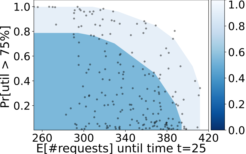
Plotting prediction regions. fig. 18 presents prediction regions on the extinction probability of the disease in the SIR model and is analogous to the tubes in fig. 5 (see figs. 26 and 31 in section 0.C.1 for plots for various other benchmarks). These regions are obtained by applying our algorithm with varying values for the cost of relaxation $\rho$ . For a confidence level of $\beta=99\%$ , the widest (smallest) tube in fig. 18 corresponds to a lower bound probability of $\mu=91.1\%$ ( $\mu=23.9\%$ ). Thus, we conclude that, with a confidence of at least $99\%$ , the curve created by the CTMC for any sampled parameter value will lie within the outermost region in fig. 18 with a probability of at least $91.1\%$ . We highlight that our approach supports more general prediction regions. We show $n=200$ solution vectors for the buffer benchmark with two measures in fig. 19 and produce regions that approach the Pareto front. For a confidence level of $\beta=99\%$ , the outer prediction region is associated with a lower bound probability of $\mu=91.1\%$ , while the inner region has a lower value of $\mu=66.2\%$ . We present more plots in section 0.C.1.

Table 2: Lower bounds

\bar{\mu}

and standard deviation (SD), vs. the observed number of

1\,000

additional solutions that indeed lie within the obtained regions.

(a) Kanban (3).

	$\beta=0.9$		$\beta=0.999$		Frequentist
$n$	$\bar{\mu}$	SD	$\bar{\mu}$	SD	Observed
100	0.862	0.000	0.798	0.000	959 $\pm$ 22.7
200	0.930	0.000	0.895	0.000	967 $\pm$ 17.4
400	0.965	0.001	0.947	0.001	984 $\pm$ 8.6
800	0.982	0.000	0.973	0.000	994 $\pm$ 3.2

(b) Railway crossing (1,1,hc).

	$\beta=0.9$		$\beta=0.999$		Frequentist
$n$	$\bar{\mu}$	SD	$\bar{\mu}$	SD	Observed
100	0.895	0.018	0.835	0.020	954 $\pm$ 26.8
200	0.945	0.007	0.912	0.008	980 $\pm$ 12.8
400	0.975	0.004	0.958	0.005	990 $\pm$ 8.3
800	0.986	0.002	0.977	0.003	995 $\pm$ 4.3

Tightness of the solution. In table 2(b) we investigate the tightness of our results. For the experiment, we set $\rho=1.1$ and solve $\mathfrak{L}_{\mathcal{U}}^{\rho}$ for different values of $n$ , repeating every experiment $10$ times, resulting in the average bounds $\bar{\mu}$ . Then, we sample $1\,000$ solutions and count the observed number of solutions contained in every prediction regions, resulting in an empirical approximation of the containment probability. Recall that for $\rho>1$ , we obtain a prediction region that contains all solutions, so this observed count grows toward $n$ . The lower bounds grow toward the empirical count for an increased $n$ , with the smallest difference (RC, $n=800$ , $\beta=0.9$ ) being as small as $0.9\%$ . Similar observations hold for other values of $\rho$ .

Handling imprecise solutions. The approximate model checker is significantly faster (see table 1 for SIR (140) and RC), at the cost of obtaining imprecise solution vectors.⁷⁷ 7 We terminate at a relative gap between upper/lower bound of the solution below 1%. For SIR (140), the sampling time is reduced from $49$ to $9\text{\,}\mathrm{min}$ , while the scenario optimization time is slightly higher at $129\text{\,}\mathrm{s}$ . This difference only grows larger with the size of the CTMC. For the larger instances of RC and HECS, computing exact solutions is infeasible at all (one HECS (2,2) sample alone takes $15\text{\,}\mathrm{min}$ ). While the bounds on the containment probability under imprecise solutions may initially be poor (see fig. 20(a), which results in $\mu=2.1\%$ ), we can improve the results significantly using the refinement scheme proposed in section 4.3. For example, fig. 20(c) shows the prediction region after refining $31$ of the $100$ solutions, which yields $\mu=74.7\%$ . Thus, by iteratively refining only the imprecise solutions on the boundary of the resulting prediction regions, we significantly tighten the obtained bounds on the containment probability.

(a)

(b)

(c)

Figure 20: Refining imprecise solution vectors (red boxes) for RC (2,2),

n=100

Table 3: Run times in [s] for solving the scenario problems for SIR and RC with

\rho=0.1

(timeout (TO) of

1

hour) for different sample sizes

n

and measures

m

(a) SIR (population 20).

$n$ / $m$	50	100	200	400	800
100	0.97	1.59	3.36	9.17	25.41
200	3.69	7.30	22.91	59.45	131.78
400	29.43	76.13	153.03	310.67	640.70
800	261.97	491.73	955.77	1924.15	TO

(b) Railway crossing (1,1,hc).

$n$ / $m$	50	100	200	400
100	1.84	3.40	8.18	24.14
200	6.35	14.56	45.09	113.09
400	34.74	96.68	203.77	427.80
800	292.32	579.09	1215.67	2553.98

Q2. Scalability

In table 3(b), we report the run times for steps (3)-(5) of our algorithm shown in fig. 15 (i.e., for solving the scenario problems, but not for computing the solution vectors in Storm). Here, we solve problem $\mathfrak{L}_{\mathcal{U}}^{\rho}$ for $\rho=0.1$ , with different numbers of samples and measures. Our approach scales well to realistic numbers of samples (up to $800$ ) and measures (up to $400$ ). The computational complexity of the scenario problems is largely independent of the size of the CTMC , and hence, similar run times are observed across the benchmarks (cf. table 1).

Q3. Comparison to baselines

We compare against two baselines: (1) Scenario optimization to analyze each measure independently, yielding a separate probabilistic guarantee on each measure. (2) A frequentist (Monte Carlo) baseline, which samples a large number of parameter values and counts the number of associated solutions within a region.

Analyzing measures independently. To show that analyzing a full set of measures at once, e.g., the complete probability curve, is essential, we compare our method to the baseline that analyzes each measure independently and combines the obtained bounds on each measure afterward. We consider the PCS benchmark with precise samples and solve $\mathfrak{L}_{\mathcal{U}}^{\rho}$ for $\rho=2$ (see table 5 in appendix 0.C for details). For $n=100$ samples and $\beta=99\%$ , our approach returns a lower bound probability of $\mu=84.8\%$ . By contrast, the naïve baseline yields a lower bound of only $4.5\%$ , and similar results are observed for different values of $n$ (cf. table 5). There are two reasons for this large difference. First, the baseline applies theorem 4.2 once for each of the $25$ measures, so it must use a more conservative confidence level of $\tilde{\beta}=1-\frac{1-\beta}{25}=0.9996$ . Second, the baseline takes the conjunction over the $25$ independent lower bounds, which drastically reduces the obtained bound.

Frequentist baseline. The comparison to the frequentist baseline on the Kanban and RC benchmarks yields the previously discussed results in table 2(b). The results in tables 1 and 3(b) show that the time spent for sampling is (for most benchmarks) significantly higher than for scenario optimization. Thus, our scenario-based approach has a relatively low cost, while resulting in valuable guarantees which the baseline does not give. To still obtain a high confidence in the result, a much larger sample size is needed for the frequentist baseline than for our approach.

7 Related Work

Several verification approaches exist to handle uncertain Markov models.

For (discrete-time) interval Markov chains (DTMCs) or Markov decision processs (MDPs), a number of approaches verify against all probabilities within the intervals [39, 32, 53, 54, 46]. Lumpability of interval CTMCs is considered in [21]. In contrast to upCTMCs, interval Markov chains have no dependencies between transition uncertainties and no distributions are attached to the intervals.

Parametric Markov models generally define probabilities or rates via functions over the parameters. The standard parameter synthesis problem for discrete-time models is to find all valuations of parameters that satisfies a specification. Techniques range from computing a solution function over the parameters, to directly solving the underlying optimization problems [28, 33, 40, 24]. Parametric CTMCs are investigated in [34, 22], but are generally restricted to a few parameters. The work [14] aims to find a robust parameter valuation in pCTMCs.

For all approaches listed so far, the results may be rather conservative, as no prior information on the uncertainties (the intervals) is used. That is, the uncertainty is not quantified and all probabilities or rates are treated equally as likely. In our approach, we do not compute solution functions, as the underlying methods are computationally expensive and usually restricted to a few parameters.

Quantified uncertainty is studied in [44]. Similarly to our work, the approach draws parameter values from a probability distribution over the model parameters and analyzes the instantiated model via model checking. However, [44] studies DTMCs and performs a frequentist (Monte Carlo) approach, cf. section 6, to compute estimates for a single measure, without prediction regions. Moreover, our approach requires significantly fewer samples, cf. the comparison in section 6.

The work in [9, 10] takes a sampling-driven Bayesian approach for pCTMCs. In particular, they take a prior on the solution function over a single measure and update it based on samples (potentially obtained via statistical model checking). We assume no prior on the solution function, and, as mentioned before, do not compute the solution function due to the expensive underlying computations.

Statistical model checking (SMC) [1, 43] samples path in stochastic models to perform model checking. This technique has been applied to numerous models [26, 27, 25, 47], including CTMCs [52, 57]. SMC analyzes a concrete CTMC by sampling from the known transition rates, whereas for upCTMC these rates are parametric.

Finally, scenario optimization [15, 20] is widely used in control theory [13] and recently in machine learning [19] and reliability engineering [49]. Within a verification context, closest to our work is [5], which considers the verification of single measures for uncertain MDPs. [5] relies on the so-called sampling-and-discarding approach [16], while we use the risk-and-complexity perspective [31], yielding better results for problems with many decision variables like we have.

8 Conclusion

This paper presents a novel approach to the analysis of parametric Markov models with respect to a set of performance characteristics. In particular, we provide a method that yields statistical guarantees on the typical performance characteristics from a finite set of samples of those parameters. Our experiments show that high-confidence results can be given based on a few hundred of samples. Future work includes supporting models with nondeterminism, exploiting aspects of parametric models such as monotonicity, and integrating methods to infer the distributions on the parameter space from observations.

References

[1] Agha, G., Palmskog, K.: A survey of statistical model checking. ACM Trans. Model. Comput. Simul. 28(1), 6:1–6:39 (2018)
[2] Allen, L.J.: A primer on stochastic epidemic models: Formulation, numerical simulation, and analysis. Infectious Disease Modelling 2(2), 128–142 (2017)
[3] Andersson, H., Britton, T.: Stochastic epidemic models and their statistical analysis, vol. 151. Springer Science & Business Media (2012)
[4] Aziz, A., Sanwal, K., Singhal, V., Brayton, R.: Model-checking continuous-time Markov chains. ACM Transactions on Computational Logic 1(1), 162–170 (2000)
[5] Badings, T.S., Cubuktepe, M., Jansen, N., Junges, S., Katoen, J.P., Topcu, U.: Scenario-based verification of uncertain parametric MDPs. CoRR abs/2112.13020 (2021)
[6] Baier, C., Haverkort, B.R., Hermanns, H., Katoen, J.P.: Model-checking algorithms for continuous-time Markov chains. IEEE Trans. Software Eng. 29(6), 524–541 (2003)
[7] Baier, C., Katoen, J.P.: Principles of Model Checking. MIT Press (2008)
[8] Bertsekas, D.P., Tsitsiklis, J.N.: Introduction to probability. Athena Scientinis (2000)
[9] Bortolussi, L., Milios, D., Sanguinetti, G.: Smoothed model checking for uncertain continuous-time Markov chains. Inf. Comput. 247, 235–253 (2016)
[10] Bortolussi, L., Silvetti, S.: Bayesian statistical parameter synthesis for linear temporal properties of stochastic models. In: TACAS. LNCS, vol. 10806, pp. 396–413. Springer (2018)
[11] Boyd, S., Vandenberghe, L.: Convex Optimization. Cambridge University Press, New York, NY, USA (2004)
[12] Budde, C.E., Dehnert, C., Hahn, E.M., Hartmanns, A., Junges, S., Turrini, A.: JANI: quantitative model and tool interaction. In: TACAS. LNCS, vol. 10206, pp. 151–168 (2017)
[13] Calafiore, G.C., Campi, M.C.: The scenario approach to robust control design. IEEE Trans. Autom. Control. 51(5), 742–753 (2006)
[14] Calinescu, R., Ceska, M., Gerasimou, S., Kwiatkowska, M., Paoletti, N.: Efficient synthesis of robust models for stochastic systems. J. Syst. Softw. 143, 140–158 (2018)
[15] Campi, M.C., Garatti, S.: The exact feasibility of randomized solutions of uncertain convex programs. SIAM J. Optim. 19(3), 1211–1230 (2008)
[16] Campi, M.C., Garatti, S.: A sampling-and-discarding approach to chance-constrained optimization: Feasibility and optimality. J. Optim. Theory Appl. 148(2), 257–280 (2011)
[17] Campi, M.C., Garatti, S.: Introduction to the scenario approach. SIAM (2018)
[18] Campi, M.C., Garatti, S.: Wait-and-judge scenario optimization. Math. Program. 167(1), 155–189 (2018)
[19] Campi, M.C., Garatti, S.: Scenario optimization with relaxation: a new tool for design and application to machine learning problems. In: CDC. pp. 2463–2468. IEEE (2020)
[20] Campi, M., Carè, A., Garatti, S.: The scenario approach: A tool at the service of data-driven decision making. Annual Reviews in Control 52, 1–17 (2021)
[21] Cardelli, L., Grosu, R., Larsen, K.G., Tribastone, M., Tschaikowski, M., Vandin, A.: Lumpability for uncertain continuous-time Markov chains. In: QEST. LNCS, vol. 12846, pp. 391–409. Springer (2021)
[22] Ceska, M., Dannenberg, F., Paoletti, N., Kwiatkowska, M., Brim, L.: Precise parameter synthesis for stochastic biochemical systems. Acta Informatica 54(6), 589–623 (2017)
[23] Ciardo, G., Tilgner, M.: On the use of Kronecker operators for the solution of generalized stochastic Petri nets. ICASE report 96-35. Institute for Computer Applications in Science and Engineering 50 (1996)
[24] Cubuktepe, M., Jansen, N., Junges, S., Katoen, J.P., Topcu, U.: Convex optimization for parameter synthesis in MDPs. IEEE Trans Autom Control pp. 1–1 (2022)
[25] D’Argenio, P.R., Hartmanns, A., Sedwards, S.: Lightweight statistical model checking in nondeterministic continuous time. In: ISoLA. LNCS, vol. 11245, pp. 336–353. Springer (2018)
[26] David, A., Larsen, K.G., Legay, A., Mikucionis, M., Poulsen, D.B.: Uppaal SMC tutorial. Int. J. Softw. Tools Technol. Transf. 17(4), 397–415 (2015)
[27] David, A., Larsen, K.G., Legay, A., Mikucionis, M., Wang, Z.: Time for statistical model checking of real-time systems. In: CAV. LNCS, vol. 6806, pp. 349–355. Springer (2011)
[28] Daws, C.: Symbolic and parametric model checking of discrete-time Markov chains. In: ICTAC. pp. 280–294. Springer (2004)
[29] Domahidi, A., Chu, E., Boyd, S.P.: ECOS: an SOCP solver for embedded systems. In: ECC. pp. 3071–3076. IEEE (2013)
[30] Garatti, S., Campi, M.C.: The risk of making decisions from data through the lens of the scenario approach. IFAC-PapersOnLine 54(7), 607–612 (2021)
[31] Garatti, S., Campi, M.: Risk and complexity in scenario optimization. Mathematical Programming pp. 1–37 (2019)
[32] Givan, R., Leach, S.M., Dean, T.L.: Bounded-parameter Markov decision processes. Artif. Intell. 122(1-2), 71–109 (2000)
[33] Hahn, E.M., Hermanns, H., Zhang, L.: Probabilistic reachability for parametric Markov models. Int. J. Softw. Tools Technol. Transf. 13(1), 3–19 (2011)
[34] Han, T., Katoen, J.P., Mereacre, A.: Approximate parameter synthesis for probabilistic time-bounded reachability. In: RTSS. pp. 173–182. IEEE CS (2008)
[35] Hartmanns, A., Klauck, M., Parker, D., Quatmann, T., Ruijters, E.: The quantitative verification benchmark set. In: TACAS. LNCS, vol. 11427, pp. 344–350. Springer (2019)
[36] Haverkort, B.R., Hermanns, H., Katoen, J.P.: On the use of model checking techniques for dependability evaluation. In: SRDS. pp. 228–237. IEEE CS (2000)
[37] Hensel, C., Junges, S., Katoen, J.P., Quatmann, T., Volk, M.: The probabilistic model checker Storm. Softw Tools Technol Transfer (2021)
[38] Hermanns, H., Meyer-Kayser, J., Siegle, M.: Multi terminal binary decision diagrams to represent and analyse continuous time Markov chains. In: 3rd Int. Workshop on the Numerical Solution of Markov Chains. pp. 188–207. Citeseer (1999)
[39] Jonsson, B., Larsen, K.G.: Specification and refinement of probabilistic processes. In: LICS. pp. 266–277. IEEE CS (1991)
[40] Junges, S., Ábrahám, E., Hensel, C., Jansen, N., Katoen, J.P., Quatmann, T., Volk, M.: Parameter synthesis for Markov models. CoRR abs/1903.07993 (2019)
[41] Katoen, J.P.: The probabilistic model checking landscape. In: LICS. pp. 31–45. ACM (2016)
[42] Kwiatkowska, M.Z., Norman, G., Parker, D.: PRISM 4.0: Verification of probabilistic real-time systems. In: CAV. LNCS, vol. 6806, pp. 585–591. Springer (2011)
[43] Legay, A., Lukina, A., Traonouez, L.M., Yang, J., Smolka, S.A., Grosu, R.: Statistical model checking. In: Computing and Software Science, LNCS, vol. 10000, pp. 478–504. Springer (2019)
[44] Meedeniya, I., Moser, I., Aleti, A., Grunske, L.: Evaluating probabilistic models with uncertain model parameters. Softw. Syst. Model. 13(4), 1395–1415 (2014)
[45] Mendelson, B.: Introduction to topology. Courier Corporation (1990)
[46] Puggelli, A., Li, W., Sangiovanni-Vincentelli, A.L., Seshia, S.A.: Polynomial-time verification of PCTL properties of MDPs with convex uncertainties. In: CAV. LNCS, vol. 8044, pp. 527–542. Springer (2013)
[47] Rao, K.D., Gopika, V., Rao, V.V.S.S., Kushwaha, H.S., Verma, A.K., Srividya, A.: Dynamic fault tree analysis using monte carlo simulation in probabilistic safety assessment. Reliab. Eng. Syst. Saf. 94(4), 872–883 (2009)
[48] Roberts, R., Neupane, T., Buecherl, L., Myers, C.J., Zhang, Z.: STAMINA 2.0: Improving scalability of infinite-state stochastic model checking. In: VMCAI. LNCS, vol. 13182, pp. 319–331. Springer (2022)
[49] Rocchetta, R., Crespo, L.G.: A scenario optimization approach to reliability-based and risk-based design: Soft-constrained modulation of failure probability bounds. Reliability Engineering & System Safety 216, 107900 (2021)
[50] Ruijters, E., Budde, C.E., Nakhaee, M.C., Stoelinga, M.I.A., Bucur, D., Hiemstra, D., Schivo, S.: FFORT: a benchmark suite for fault tree analysis. In: ESREL (2019)
[51] Ruijters, E., Stoelinga, M.I.A.: Fault tree analysis: A survey of the state-of-the-art in modeling, analysis and tools. Comput. Sci. Rev. 15, 29–62 (2015)
[52] Sen, K., Viswanathan, M., Agha, G.: On statistical model checking of stochastic systems. In: CAV. LNCS, vol. 3576, pp. 266–280. Springer (2005)
[53] Sen, K., Viswanathan, M., Agha, G.: Model-checking Markov chains in the presence of uncertainties. In: TACAS. pp. 394–410. Springer (2006)
[54] Skulj, D.: Discrete time Markov chains with interval probabilities. Int. J. Approx. Reason. 50(8), 1314–1329 (2009)
[55] Volk, M., Junges, S., Katoen, J.P.: Fast dynamic fault tree analysis by model checking techniques. IEEE Trans. Ind. Informatics 14(1), 370–379 (2018)
[56] Wijesuriya, V.B., Abate, A.: Bayes-adaptive planning for data-efficient verification of uncertain Markov decision processes. In: QEST. LNCS, vol. 11785, pp. 91–108. Springer (2019)
[57] Younes, H.L.S., Simmons, R.G.: Statistical probabilistic model checking with a focus on time-bounded properties. Inf. Comput. 204(9), 1368–1409 (2006)

Appendix 0.A Additional Examples

In the following example, we discuss the results shown in fig. 11 in more detail.

Example 4

We consider the Kanban manufacturing system benchmark from [23] with a Gaussian distribution over the parameters. In fig. 11, we present $n=25$ solution vectors for two expected cost measures. We use these solutions in problem $\mathfrak{L}^{\rho}_{\mathcal{U}}$ in eq. 2, and solve for $\rho=2$ , $0.4$ , and $0.15$ . We show the three resulting prediction regions in fig. 11. For $\rho=2$ , the prediction region contains all vectors, while for a lower cost of relaxation $\rho$ , more vectors are left outside. ∎

Appendix 0.B Proofs

0.B.1 Proof of theorem 3.1

The proof of theorem 3.1 is based on [20], which states that for a complexity $c^{*}_{\rho}$ and for $\eta(c^{*}_{\rho})$ the smallest positive solution to eq. 4, it holds that

\amsmathbb{P}^{n}\Big\{V\big(R^{*}_{\rho})\leq 1-\eta(c^{*}_{\rho})\Big\}\geq\beta,

(7)

where $V(R^{*}_{\rho})$ is the so-called violation probability, which is defined as

V(R^{*}_{\rho})=\textnormal{Pr}\{u\in\mathcal{V}_{\mathcal{M}}\,\colon\,\mathsf{sol}(u)\notin R^{*}_{\rho}\}.

(8)

Observe that $\mathsf{contain}(R^{*}_{\rho})+V(R^{*}_{\rho})=1$ . Thus, we rewrite eq. 7 as

\amsmathbb{P}^{n}\Big\{\mathsf{contain}(R^{*}_{\rho})\geq\eta(c^{*}_{\rho})\Big\}\geq\beta.

(9)

Note that $\eta(c)$ is monotonically decreasing in $c$ [30], so for any $d^{*}_{\rho}\geq c^{*}_{\rho}$ , we have $\eta(d^{*}_{\rho})\leq\eta(c^{*}_{\rho})$ . Hence, eq. 9 also implies eq. 3, which concludes the proof.

0.B.2 Proof of lemma 1

Recall from the proof of theorem 3.1 that for $\eta(c^{*}_{\rho})$ the solution to eq. 4, where $c^{*}_{\rho}$ is the true complexity of problem $\mathfrak{L}^{\rho}_{\mathcal{U}}$ , it holds that

\amsmathbb{P}^{n}\Big\{\mathsf{contain}\big(R^{*}_{\rho}\big)\geq\eta(c^{*}_{\rho})\Big\}\geq\beta.

(10)

Observe that for any two sets $R^{*}_{\rho}\subseteq R$ , we have $\mathsf{contain}\big(R\big)\geq\mathsf{contain}\big(R^{*}_{\rho}\big)$ . Moreover, recall that $\eta(c)$ is monotonically decreasing in $c$ (as also observed visually from fig. 14), and thus, the condition $c^{*}_{\rho}\leq d$ implies that $\eta(d)\leq\eta(c_{\rho}^{*})$ . Hence, under the proposed conditions, we rewrite eq. 10 as the right-hand side of eq. 5, which concludes the proof.

0.B.3 Proof of theorem 4.1

The one-dimensional case. Let us first consider the case for one dimension, i.e., one measure. Recall from example 1 that for precise solutions in 1D, the outermost two samples (labeled A and F) are relaxed under the (unique) optimal solution if $\rho<1$ , samples B and E if $\rho<\frac{1}{2}$ , etc. Denote by $\mathsf{sol}^{-}(u)_{r}=\mathsf{sol}^{-,\varphi_{r}}_{\mathcal{M}[u]}$ and $\mathsf{sol}^{+}(u)_{r}=\mathsf{sol}^{+,\varphi_{r}}_{\mathcal{M}[u]}$ the $r$ -th entries of the respective imprecise solution vectors, i.e., the (upper and lower bound) solutions for measure $\varphi_{r}\in\Phi$ and the CTMC created by sample $u\in\mathcal{V}_{\mathcal{M}}$ . In formalizing the relationship between the value of $\rho$ and whether a sample is relaxed, we state the following definition:

Definition 9.

Let $r\leq|\Phi|$ . For any $(\mathsf{sol}(u_{i})^{-},\mathsf{sol}(u_{i})^{+})$ , we define $\mathsf{num}^{+}_{\geq}(u_{i})_{r}\in\{1,\ldots,n\}$ and $\mathsf{num}^{-}_{\leq}(u_{i})_{r}\in\{1,\ldots,n\}$ as the number of samples whose upper bound is at least $\mathsf{sol}^{+}(u_{i})$ (or at most $\mathsf{sol}^{-}(u_{i})$ ), when projected to dimension $r$ :

	$\displaystyle\mathsf{num}^{+}_{\geq}(u_{i})_{r}$	$\displaystyle=\big\|\{u_{j}\in\mathcal{V}_{\mathcal{M}}\,\colon\,\mathsf{sol}^{+}(u_{j})_{r}\geq\mathsf{sol}^{+}(u_{i})_{r}\}\big\|$
	$\displaystyle\mathsf{num}^{-}_{\leq}(u_{i})_{r}$	$\displaystyle=\big\|\{u_{j}\in\mathcal{V}_{\mathcal{M}}\,\colon\,\mathsf{sol}^{-}(u_{j})_{r}\leq\mathsf{sol}^{-}(u_{i})_{r}\}\big\|.$

Figure 21: The upper bounds of five imprecise solutions and their values of

\mathsf{sol}^{+}_{\geq}(u).

fig. 21 shows an extended version of fig. 16 which also presents the values of $\mathsf{num}^{+}_{\geq}(u)$ for the upper bounds on the imprecise solutions. The following lemma then characterizes the relaxed solutions:

Lemma 3

An imprecise solution $(\mathsf{sol}^{-}(u),\mathsf{sol}^{+}(u)),\,u\in\mathcal{V}_{\mathcal{M}}$ is not contained in the prediction region $[\underaccent{\bar}{x}^{\prime}_{\rho},\bar{x}^{\prime}_{\rho}]$ of $\mathfrak{G}^{\rho}_{\mathcal{U}}$ , projected to dimension $p\leq|\Phi|$ , if

\rho<\min\Big\{\mathsf{num}^{+}_{\geq}(u)_{p},\,\,\mathsf{num}^{-}_{\leq}(u)_{p}\Big\}^{-1}.

(11)

For precise solutions, there is no distinction between $\mathsf{sol}^{-}(u_{i})$ and $\mathsf{sol}^{+}(u_{i})$ , and definition 9 yields the sets $\mathsf{num}_{\geq}(u_{i})_{r}$ and $\mathsf{num}_{\leq}(u_{i})_{r}$ . We can check whether a precise solution $\mathsf{sol}(u)$ is contained in the prediction region $[\underaccent{\bar}{x}^{*}_{\rho},\bar{x}^{*}_{\rho}]$ to $\mathfrak{L}^{\rho}_{\mathcal{U}}$ by replacing $\mathsf{num}^{+}\to\mathsf{num}$ and $\mathsf{num}^{-}\to\mathsf{num}$ in eq. 11.

Proof of theorem 4.1 (part I).

We proof the theorem by contradiction for the 1-dimensional case, and we generalize afterward. In a single dimension, $[\underaccent{\bar}{x}^{*}_{\rho},\bar{x}^{*}_{\rho}]\not\subseteq[\underaccent{\bar}{x}^{\prime}_{\rho},\bar{x}^{\prime}_{\rho}]$ requires that either $\underaccent{\bar}{x}^{*}_{\rho}<\underaccent{\bar}{x}^{\prime}_{\rho}$ or $\bar{x}^{*}_{\rho}>\bar{x}^{\prime}_{\rho}$ . First consider the upper bounds $\bar{x}^{\prime}_{\rho}$ and $\bar{x}^{*}_{\rho}$ , which we can make explicit using lemma 3:

	$\displaystyle\bar{x}^{\prime}_{\rho}$	$\displaystyle=\max\big\{\mathsf{sol}^{+}(u),u\in\mathcal{V}_{\mathcal{M}}\,\colon\,\mathsf{num}^{+}_{\geq}(u)>\rho^{-1}\big\}$		(12)
	$\displaystyle\bar{x}^{*}_{\rho}$	$\displaystyle=\max\big\{\mathsf{sol}(u),u\in\mathcal{V}_{\mathcal{M}}\,\colon\,\mathsf{num}_{\geq}(u)>\rho^{-1}\big\}.$		(13)

For $\bar{x}^{*}_{\rho}>\bar{x}^{\prime}_{\rho}$ to hold, the maximum $\mathsf{num}_{\geq}(u)>\rho^{-1}$ (i.e., the highest precise solution for which there are more than $\rho^{-1}$ solutions at least as high) must exceed $\mathsf{num}^{+}_{\geq}(u)>\rho^{-1}$ (the highest imprecise upper bound solution for which there are more than $\rho^{-1}$ imprecise upper bound solutions at least as high). This can only be true if the number of samples for which $\mathsf{sol}(u)>\bar{x}^{\prime}$ is higher than the number for which $\mathsf{sol}^{+}(u)>\bar{x}^{\prime}$ . However, by construction, $\mathsf{sol}(u)\leq\mathsf{sol}^{+}$ , so this is impossible, and thus, it holds that $\bar{x}^{*}_{\rho}\leq\bar{x}^{\prime}_{\rho}$ . While omitted for brevity, the proof that the lower bound $\underaccent{\bar}{x}^{*}_{\rho}\geq\bar{x}^{\prime}_{\rho}$ follows analogous to the upper bound. ∎

The multi-dimensional case.

Lemma 4

Problem $\mathfrak{G}_{\mathcal{U}}^{\rho}$ can be decomposed into an independent problem for every dimension $1,\ldots,m$ , with $m=|\Phi|$ the number of measures in $\Phi$ .

lemma 4 holds because the objective eq. 2a is additive and all constraints for all measures eq. 2b are independent. Thus, we can equivalently solve problem $\mathfrak{L}_{\mathcal{U}}^{\rho}$ for all $m$ measures separately.

Proof of theorem 4.1 (part II).

We now generalize the result to multiple dimensions. lemma 4 states that for rectangular prediction regions, problems $\mathfrak{L}^{\rho}_{\mathcal{U}}$ and $\mathfrak{G}^{\rho}_{\mathcal{U}}$ can be solved for each dimension separately. As such, we obtain an element-wise inequality $\underaccent{\bar}{x}^{\prime}_{\rho}\leq\underaccent{\bar}{x}^{*}_{\rho}\leq\bar{x}^{*}_{\rho}\leq\bar{x}^{*}_{\rho}$ , which also implies that $[\underaccent{\bar}{x}^{*}_{\rho},\bar{x}^{*}_{\rho}]\subseteq[\underaccent{\bar}{x}^{\prime}_{\rho},\bar{x}^{\prime}_{\rho}]$ , so the claim in follows. ∎

0.B.4 Proof of Theorem 4.2

Before providing the proof, we state the following useful lemma about surely noncritical samples:

Lemma 5

Any surely noncritical sample cannot be in the (smallest) critical set, defined in definition 7.

Proof.

Recall from definition 7 that a sample may (potentially) be critical if it is either outside or on the boundary of the prediction region $[\underaccent{\bar}{x}^{*}_{\rho},\bar{x}^{*}_{\rho}]$ . While the boundary of the prediction region $[\underaccent{\bar}{x}^{*}_{\rho},\bar{x}^{*}]$ is unknown, it cannot be smaller than the inner rectangle $\mathcal{I}$ defined in definition 8. By construction, any surely noncritical sample is a subset of this set $\mathcal{I}$ . Hence, any surely noncritical sample cannot be in the (smallest) critical set, and the claim follows. ∎

The proof of theorem 4.2 now follows almost directly from lemma 5. The complexity is the cardinality of the smallest critical set, which cannot contain any surely noncritical sample, as stated by lemma 5. Hence, it follows that $n-|X|=|\mathcal{U}_{n}\setminus\mathcal{X}|$ , where $\mathcal{X}$ is the set of surely noncritical samples, which concludes the proof.

Appendix 0.C Detailed Benchmark Overview and Results

In this appendix, we illustrate on two specific benchmarks how we convert a pCTMC into a upCTMC by equipping its parameters with a probability distribution. We omit details on the other benchmarks for brevity. Thereafter, we present the full benchmark statistics in table 4, as well as more graphical outputs of our implementation in figs. 26 and 31.

Epidemic modeling. We consider the classical SIR infection model [3] of an infectious disease spreading through a population. The factored state $s=(\bar{S},\bar{I},\bar{R})$ of this CTMC counts the susceptible, infected, and recovered populations. Infections and recoveries (we assume that immunization is permanent) occur based on the following parametric rules that depend on parameters $\lambda_{i}$ and $\lambda_{r}$ :

\displaystyle\textbf{Infection:\,\,}S+I\xrightarrow{\lambda_{i}\cdot\bar{S}\cdot\bar{I}}I+I,\quad\quad\textbf{Recovery:\,\,}I\xrightarrow{\lambda_{r}\cdot\bar{I}}R.

In the classical SIR model, $\lambda_{i}$ and $\lambda_{r}$ are assumed to be known precisely, while we consider the parameters $\lambda_{i}=\mathcal{N}(0.05,0.002)$ and $\lambda_{r}=\mathcal{N}(0.04,0.002)$ to be normally distributed (recall that we only use samples from these distributions). We define a set $\Phi=\{\varphi_{100+100i}\,\colon\,i=\frac{1}{m},\frac{2}{m},\ldots,\frac{m-1}{m},1\}$ of $m$ measures, where $\varphi_{t}$ is the probability that the disease becomes extinct between time $100$ and $t$ :

\varphi_{t}=(\bar{I}>0)\textbf{U}_{[100,t]}(\bar{I}=0).

(14)

Buffer system. We augment the producer-consumer buffering system from [14]. We equip the six parameters of this pCTMC by uniform probability distributions with their domains specified below. This pCTMC models the transfer of requests from a producer (at a rate of $\lambda_{g}\in[32,38]$ ) to consumers who consume them (at a rate of $\lambda_{c}\in[27,33]$ ). The requests are sent at a rate of $\lambda_{t}\in[27,33]$ , via either a slow or a fast buffer, with probabilities of $0.6$ and $0.4$ , respectively. While being faster, the fast buffer is less reliable than the slow buffer (it loses requests with a probability $\lambda_{\text{loss}}\in[0.025,0.075]$ ), and has a smaller capacity. Requests from the slow buffer are transferred to the fast buffer with a probability proportional to the occupancy. The transmission rate of the slow buffer is $\lambda_{\text{slow}}\in[5,15]$ ; the rate of the fast buffer is $\lambda_{\delta}\in[5,15]$ higher. We consider two measures: (1) the expected transferred requests until time $25$ , and (2) the probability that the utilization of both buffers is above 75% within the time $[20,25]$ .

0.C.1 Detailed results

The complete overview of the statistics of all benchmarks is shown in table 4. Running polling (15) for $n=200$ samples led to a timeout, due to the very high sampling times (sampling 100 solutions already takes over 3.5 hours). The obtained prediction regions for eight benchmarks (under precise solutions) are presented in figs. 26 and 31. These plots demonstrate the wide applicability and effectiveness of our method on a large variety of benchmarks.

Table 4: Model sizes and run times for all benchmarks (the sampling time in Storm is reported per

100

CTMCs).

		Model size			Storm run time [s]		Scen.opt. time [s]
benchmark	$\|\Phi\|$	#pars	#states	#trans	Init.	Sample ( $\times 100$ )	$N=100$	$N=200$
SIR (20)	26	2	216	396	0.02	2.93	2.44	10.18
SIR (60)	26	2	1 876	3 636	0.06	121.65	16.91	52.57
SIR (100)	26	2	5 136	10 076	0.15	829.47	19.35	62.74
SIR (100)^a	26	2	5 136	10 076	0.15	191.30	27.45	137.76
SIR (140)	26	2	9 996	19 716	0.29	2947.29	18.26	63.27
SIR (140)^a	26	2	9 996	19 716	0.29	544.27	25.11	129.66
Kanban (3)	4	13	58 400	446 400	4.42	46.95	2.28	6.69
Kanban (5)	4	13	2 546 432	24 460 016	253.39	4363.63	2.03	5.94
polling (3)	2	2	36	84	0.02	0.08	2.35	7.31
polling (9)	2	2	6 912	36 864	0.64	22.92	2.13	6.66
polling (15)	2	2	737 280	6 144 000	3 908.13	9 509.22	2.07	–
buffer	2	6	5 632	21 968	0.48	20.70	1.21	4.15
tandem (15)	2	5	496	1 619	0.03	82.01	1.67	5.36
tandem (31)	2	5	2 016	6 819	0.11	862.41	5.19	24.30
embed. (64)	3	6	55 868	235 793	3.31	8.07	3.97	12.69
embed. (256)	3	6	218 108	920 657	18.04	33.40	3.99	13.03
pcs	25	6	2 501	14 985	0.03	37.20	3.51	13.07
rbc	40	6	2 269	12 930	0.01	1.40	5.27	16.88
dcas	25	10	64	202	0.01	0.48	3.10	10.88
rc (1,1)	25	21	8 401	49 446	27.20	74.90	5.75	20.34
rc (1,1)^a	25	21	n/a^b	n/a^b	0.02	2.35	29.23	150.61
rc (2,2)^a	25	29	n/a^b	n/a^b	0.03	27.77	24.86	132.63
hecs (2,1)	25	5	118 945	1 018 603	0.04	6.42	3.87	13.18
hecs (2,1)^a	25	5	n/a^b	n/a^b	0.02	9.83	26.78	145.77
hecs (2,2)^a	25	24	n/a^b	n/a^b	0.02	194.25	33.06	184.32

a

Computed using approximate model checking up to a relative gap between upper
bound $\mathsf{sol}^{+}(u)$ and lower bound $\mathsf{sol}^{-}(u)$ below $1\%$ for every sample $u\in\mathcal{V}_{\mathcal{M}}$ .
b

Model size is unknown, as the approximation does not build the full state-space.

Analyzing measures independently.

Table 5: Obtained bounds (for the PCS fault tree) on the containment probability for our approach and the baseline that analyzes each measure independently.

	$n=100$		$n=200$		$n=400$		$n=800$
Method	$\beta=0.9$	$\beta=0.999$	$\beta=0.9$	$\beta=0.999$	$\beta=0.9$	$\beta=0.999$	$\beta=0.9$	$\beta=0.999$
Our approach	0.908	0.848	0.937	0.903	0.976	0.960	0.984	0.975
Baseline	0.045	0.010	0.212	0.103	0.461	0.322	0.679	0.567

table 5 presents the full comparison on the PCS benchmark between our approach and the baseline scenario approach that analyzes each measure independently. In this table, we report the average lower bounds (over 10 iterations) on the containment probability, for different sample sizes $n=100,\ldots,800$ and confidence levels $\beta$ . For the two main reasons for the significant difference in the tightness of the containment probability, we refer to section 6 in the main paper.

Sampling-Based Verification of CTMCs with Uncertain Rates Thanks: This work has been partially funded by NWO under the grant PrimaVera, number NWA.1160.18.238, and by EU Horizon 2020 project MISSION, number 101008233.

Abstract

1 Introduction

2 Problem Statement

Definition 1 (pCTMC).

Definition 2 (Solution function).

Definition 3 (Probability curve).

Definition 4 (upCTMC).

Definition 5 (Containment probability).

Definition 6 (Prediction region for a probability curve).

3 Precise Sampling-Based Prediction Regions

3.1 Constructing prediction regions

Assumption 1.

Example 1

Remark 1.

3.2 Bounding the containment probability

Definition 7 (Complexity).

Example 2

Theorem 3.1

Example 3

3.3 An algorithm for computing prediction regions

4 Imprecise Sampling-Based Prediction Regions

Lemma 1

4.1 Prediction regions on imprecise solutions

Theorem 4.1

4.2 Computing the complexity

Lemma 2

Proof.

Definition 8.

Theorem 4.2

4.3 Solution refinement scheme

5 Batch Verification for CTMCs

6 Experiments

Q1. Applicability

Q2. Scalability

Q3. Comparison to baselines

7 Related Work

8 Conclusion

References

Appendix 0.A Additional Examples

Example 4

Appendix 0.B Proofs

0.B.1 Proof of theorem 3.1

0.B.2 Proof of lemma 1

0.B.3 Proof of theorem 4.1

Definition 9.

Lemma 3

Proof of theorem 4.1 (part I).

Lemma 4

Proof of theorem 4.1 (part II).

0.B.4 Proof of Theorem 4.2

Lemma 5

Proof.

Appendix 0.C Detailed Benchmark Overview and Results

0.C.1 Detailed results

Sampling-Based Verification of CTMCs
with Uncertain Rates Thanks: This work has been partially funded by NWO under the grant PrimaVera, number NWA.1160.18.238, and by EU Horizon 2020 project MISSION, number 101008233.