Fast consensus of high-order multi-agent systems

Jiahao Dai Jing-Wen Yi Li Chai Thanks: This work was supported by the National Natural Science Foundation of China (62173259, 62176192, 61625305 and 61701355). Thanks: Jiahao Dai and Jing-Wen Yi are with the Engineering Research Center of Metallurgical Automation and Measurement Technology, Wuhan University of Science and Technology, Wuhan 430081, China. e-mail: daijiahao@wust.edu.cn; yijingwen@wust.edu.cn. Thanks: Li Chai is with the College of Control Science and Engineering, Zhejiang University, Hangzhou 310027, China. e-mail: chaili@zju.edu.cn.

Abstract

In this paper, the fast consensus problem of high-order multi-agent systems under undirected topologies is considered. The direct link between the consensus convergence rate and the control gains is established. An accelerated consensus algorithm based on gradient descent is proposed to optimize the convergence rate. By applying the Routh-Hurwitz stability criterion, the lower bound on the convergence rate is derived, and explicit control gains are derived as the necessary condition to achieve the optimal convergence rate. Moreover, a protocol with time-varying control gains is designed to achieve the finite-time consensus. Explicit formulas for the time-varying control gains and the final consensus state are given. Numerical examples and simulation results are presented to illustrate the obtained theoretical results.

Index Terms:

Multi-agent systems; high-order; fast consensus; convergence rate; finite-time consensus.

I Introduction

Consensus is a fundamental problem in distributed coordination, which has been extensively studied in [1, 2, 3, 4]. The main purpose of consensus is to design a control protocol, which use the local information between an agent and its neighbors, such that the states of all agents can reach a common value over time.

The convergence rate is an important indicator to evaluate the consensus performance. There are many methods to accelerate the convergence rate, which can be roughly summarized as: optimizing the weight matrix [5, 6, 7], using the time-varying control [8, 9, 10], and introducing the agent’s memory [11, 12, 13]. Recently, Yi et al. [14] gave an explicit formula for the optimal convergence rate of first-order MASs from the perspective of graph signal frequency domain filtering, and Dai et al. [15] proposed a general control protocol with memory to accelerate the consensus of first-order MASs.

Most of the above methods to optimize the convergence rate are considered in the first-order system. However, a broad class of systems have multiple degrees of freedom in practical applications, where the input-output relationship needs to be illustrated by higher-order dynamics [16, 17, 18, 19, 20]. Then some researchers explored the convergence rate of higher-order MASs. Li et al. [21] studied a consensus algorithm for MASs with double-integrator dynamics, and proved that the finite-time consensus can be achieved by using Lyapunov stability theory. Under assumptions that the system matrix is controllable and the product of the unstable eigenvalues of the open-loop system matrix has a upper bound, You et al. [22] provided a lower bound of the optimal convergence rate for high-order discrete-time MASs. Eichler et al. [23] proposed a protocol for the consensus of MASs with discrete-time double-integrator dynamics, and derived the optimal control gain by minimizing the largest eigenvalue modulus of the closed-loop system matrix. Parlangeli et al. [24] proposed a control protocol in high-order continuous-time leader-follower networks, and indicated that the convergence can be achieved arbitrarily fast by allocating all the eigenvalues of the closed-loop system matrix.

In this paper, the fast consensus problem of high-order MASs is considered. Control protocols with constant control gains and time-varying control gains are used to achieve the accelerated asymptotic consensus and the finite-time consensus, respectively. The main contributions of this paper are summarized as follows.
(i) The necessary and sufficient condition for high-order MASs to achieve asymptotic consensus is given. The direct link between the consensus convergence rate and the control gains is established.
(ii) The accelerated asymptotic consensus problem is transformed into an optimization problem of the convergence rate, and an accelerated consensus algorithm based on gradient descent is proposed to solve this problem. By applying the Routh-Hurwitz stability criterion, the lower bound on the convergence rate is given, and explicit control gains are derived as the necessary condition to achieve the optimal convergence rate.
(iii) The explicit formula of time-varying control gains to achieve the finite-time consensus is derived by applying the Cayley-Hamilton theorem. It is shown that the step to achieve consensus is determined by the system’s order and the number of distinct non-zero eigenvalues of Laplacian.

The rest of this paper is organized as follows. In Section II, the problem statement are presented. Section III proposes some consensus conditions, designs an accelerated consensus algorithm to accelerate consensus, and derives a lower bound on the convergence rate. Section IV introduces a time-varying control protocol to achieve the finite-time consensus, and gives explicit formulas for the time-varying control gains. In Section V, numerical examples are given to verify the theoretical analysis. Finally, Section VI concludes this paper.

Notations: The notations used in this paper are standard. The notation $diag\{\,\cdots\}$ denotes a block-diagonal matrix. $\mathbb{R}^{n}$ and $\mathbb{R}^{m\times n}$ are the sets of column vectors of dimension ${n}$ and matrices of dimension ${m\times n}$ with real elements, respectively. ${\left\|\,\cdot\,\right\|_{2}}$ denotes the Euclidean norm. The symbol $\otimes$ stands for Kronecker product. The symbol $C_{p}^{q}=\frac{{p!}}{{q!(p-q)!}}$ denotes the number of $q$ -combinations from a given set of $p$ elements. Without special explanation, $\bm{0}$ and $I$ represent the zero matrix and identity matrix with appropriate dimensions, and $\bm{1}$ denotes the vector of all ones.

II Preliminaries

II-A Graph Theory

The interactions among agents are modeled as an undirected graph $\mathcal{G\!=\!(V,E,A)}$ , where $\mathcal{V}\!=\!\{\text{v}_{1},\text{v}_{2},\cdots,\text{v}_{N}\}$ presents a set of agents or nodes, $\mathcal{E\!\subseteq\!V\times V}$ presents a set of edges, and $\mathcal{A}\!=\![a_{ij}]\!\in\!\mathbb{R}^{N\!\times\!N}$ presents the weighted adjacency matrix. The adjacency element $a_{ij}\!=\!a_{ji}\!>\!0$ if the edge between node $i$ and $j$ satisfies $e_{ij}\in\mathcal{E}$ . Denote the set of neighbors of node as ${\mathcal{N}_{i}}\!=\!\left\{{{\text{v}_{j}}\in\mathcal{V}:({\text{v}_{i}},{\text{v}_{j}})\in\mathcal{E}}\right\}$ . Define the Laplacian matrix of $\mathcal{G}$ as $\mathcal{L=D-A}$ , where $\mathcal{D}\!=\!diag\{d_{1},\cdots,d_{N}\}$ and ${d_{i}}\!=\!\sum\nolimits_{j=1}^{N}{{a_{ij}}}$ . For a connected graph, all the eigenvalues of $\mathcal{L}$ are real in an ascending order as $0\!=\!{\lambda_{1}}\!<\!{\lambda_{2}}\!\leq\!\cdots\!\leq\!{\lambda_{N}}$ .

Lemma 1.

[25] For any connected undirected graph $\mathcal{G}$ , its Laplacian matrix has the following properties.
(i) $\mathcal{L}$ has the spectral decomposition ${\mathcal{L}=V\Lambda V^{T}}$ , where $\Lambda\!=\!diag\{\lambda_{1},\lambda_{2},\cdots,\lambda_{N}\}$ and $V\!=\![\bm{v}_{1},\bm{v}_{2},\cdots,\bm{v}_{N}]\!\in\!\mathbb{R}^{N\times N}$ .
(ii) Zero is a single eigenvalue of $\mathcal{L}$ , and the corresponding eigenvector is $\bm{v}_{1}\!=\!\frac{1}{\sqrt{N}}\bm{1}$ .

II-B Problem Formulation

Agents might only be able to interact with their neighbors intermittently rather than continuously because digital signals communicate in discrete time. A discrete-time high-order MAS containing $N$ agents with order $n\geq 1$ is considered as follows.

\begin{array}[]{*{20}{l}}{\begin{array}[]{*{20}{l}}{x_{i}^{(1)}(k+1)=x_{i}^{(1)}(k)+x_{i}^{(2)}(k)\cdot\tau,}\\ {x_{i}^{(2)}(k+1)=x_{i}^{(2)}(k)+x_{i}^{(3)}(k)\cdot\tau,}\\ \;\;\;\;\;\;\;\;\;\;\;\;\;\;\;\;\;\;\;\vdots\\ {x_{i}^{(n)}(k+1)=x_{i}^{(n)}(k)+{u_{i}}(k)\cdot\tau,}\end{array}}&\begin{array}[]{l}i=1,2,\ldots,N,\\ l=1,2,\ldots,n.\end{array}\end{array}

(1)

where $x_{i}^{(l)}(k)\in\mathbb{R}$ represents the $l$ -order state of the agent $i$ , $u_{i}(k)\in\mathbb{R}$ is the control input, and $\tau\in\mathbb{R}^{+}$ denotes the sampling period.

Let $\bm{x}_{i}(k)=[x_{i}^{(1)}(k),\cdots,x_{i}^{(n)}(k)]^{T}$ and rewrite system (1) into a matrix form

\begin{array}[]{*{20}{c}}{{{\bm{x}}_{i}}(k+1)=A{\bm{x}_{i}}(k)+B{u_{i}}(k),}&{i=}\end{array}1,2,\ldots,N,

(2)

where

A=\left[{\begin{array}[]{*{20}{c}}{\;1\;}&{\;\tau\;}&&\\ &{\;1\;}&{\;\ddots\;}&\\ &&{\;\ddots\;}&{\;\tau\;}\\ &&&{\;1\;}\end{array}}\right],B=\left[{\begin{array}[]{*{20}{c}}0\\ \vdots\\ 0\\ \tau\end{array}}\right].

(3)

Remark 1.

Ma et al. [26] studied the consensus problem of high-order MASs, indicating that the state of each agent converges to zero without taking any control when the open-loop system is stable. It means that studying the consensus of open-loop stable systems is of little significance. For an unstable open-loop system, it is usually necessary to make some assumptions to achieve consensus. However, these assumptions make the conclusions obtained conservative. For example, References [22, 27] limit the range of eigenratio $\lambda_{2}/\lambda_{N}$ . In fact, for an unstable open-loop system, each agent can use a local controller ${u_{i}}(k)=K_{i}{x_{i}}(k)$ for pole-placement, and make the open-loop system marginally stable. Then the neighbor information can be utilized to achieve consensus. Therefore, the marginally stable open-loop system considered in [18, 16, 19] and this paper is not loss of generality. Instead, we think it is more suitable for practical applications.

Definition 1.

Consider the high-order MAS (1) with arbitrary initial value.
(i) Consensus is said to be reached asymptotically if

\begin{array}[]{*{20}{l}}{\mathop{\lim}\limits_{k\to\infty}\left[{x_{i}^{(l)}(k)-x_{j}^{(l)}(k)}\right]=0},\\ i,j=1,2,\cdots,N,\,\,l=1,2,\cdots,n.\end{array}

(ii) Consensus is said to be reached at step $\rm{T}$ if

\begin{array}[]{*{20}{c}}{x_{i}^{(l)}(k)-x_{j}^{(l)}(k)=0},\,\,i,j=1,2,\cdots,N,\,\,l=1,2,\cdots,n\end{array}

holds for any $k\geq\rm{T}$ .

This paper aims to design control protocols and corresponding control gains to achieve the accelerated asymptotic consensus and the finite-time consensus.

III Accelerated asymptotic consensus by a time-invariant control protocol

In this section, the accelerated asymptotic consensus problem of high-order MASs is studied.

Consider the following time-invariant control protocol

{u_{i}}(k)=K\sum\limits_{j\in{\mathcal{N}_{i}}}{{a_{ij}}({\bm{x}_{j}}(k)-{\bm{x}_{i}}(k))},

(4)

where $K=[{K_{1}},{K_{2}},\cdots,{K_{n}}]\in\mathbb{R}^{1\times n}$ denotes the control gain, and ${\bm{x}_{i}}(k)={[x_{i}^{(1)}(k),\cdots,x_{i}^{(n)}(k)]^{T}}$ . Denote $\bm{x}(k)=[\bm{x}_{1}(k)^{T},\bm{x}_{2}(k)^{T},\cdots,\bm{x}_{N}(k)^{T}]^{T}$ . The system (2) can be written as

\bm{x}(k+1)=({I_{N}}\otimes A-\mathcal{L}\otimes BK)\bm{x}(k).

(5)

Let $H({\lambda_{i}},K)=A\!-\!{\lambda_{i}}BK$ . According to ${\mathcal{L}=V\Lambda V^{T}}$ , we have

$\displaystyle\bm{x}(k)=$	$\displaystyle(V\otimes{I_{n}})diag\{A,H({\lambda_{2}},K),\ldots,H({\lambda_{N}},K)\}$	(6)
	$\displaystyle({V^{T}}\otimes{I_{n}})\bm{x}(k-1)$
$\displaystyle=$	$\displaystyle\frac{1}{N}(\bm{1}_{N}\otimes{I_{n}}){A^{k}}({\bm{1}^{T}_{N}}\otimes{I_{n}})\bm{x}(0)$
	$\displaystyle+\sum\limits_{i=2}^{N}{({\bm{v_{i}}}\otimes{I_{n}}){H^{k}}({\lambda_{i}},K)(\bm{v_{i}}^{T}\otimes{I_{n}})x(0)}.$

Note that $\frac{1}{N}(\bm{1}_{N}\otimes{I_{n}}){A^{k}}({\bm{1}^{T}_{N}}\otimes{I_{n}})\bm{x}(0)$ in (6) is the part to achieve consensus. We need to design the control gain $K$ so that

\mathop{\lim}\limits_{k\to\infty}\sum\limits_{i=2}^{N}{(\bm{v_{i}}\otimes{I_{n}}){H^{k}}({\lambda_{i}},K)(\bm{v_{i}}^{T}\otimes{I_{n}})x(0)}=0.

The convergence rate is determined by the eigenvalue of $H({\lambda_{i}},K)$ with the largest modulus. Thus, the consensus convergence rate can be defined as [22]

{r}=r(K)=\mathop{\max}\limits_{{\lambda_{i}}\in\left\{{{\lambda_{2}},\ldots,{\lambda_{N}}}\right\}}\rho\left({H({\lambda_{i}},K)}\right),

(7)

where $\rho\left(\cdot\right)$ denotes spectral radius.

Remark 2.

Denote

\bm{e}(k)=\bm{x}(k)-\frac{1}{N}({\bm{1}_{N}}\otimes{I_{n}}){A^{k}}(\bm{1}_{N}^{T}\otimes{I_{n}})\bm{x}(0).

According to equation (6), we have $\mathop{\lim}\limits_{k\to\infty}{\left\|{\bm{e}(k)}\right\|_{2}}\sim{\rm{O}}({r^{k}})$ . Note that time $t=k\tau$ at step $k$ . Then $\mathop{\lim}\limits_{t\to\infty}{\left\|{\bm{e}(t)}\right\|_{2}}\sim{\rm{O}}({r^{t/\tau}})$ . A smaller $r$ or $\tau$ can get faster convergence of consensus.

In this section, our goal is to design the control gain $K$ to make the convergence rate $r$ as small as possible.

III-A Conditions for consensus

In this subsection, the necessary and sufficient condition for higher-order MASs to achieve asymptotic consensus is proposed.

Lemma 2.

(Schur Complement [28]) Given a matrix

M=\left[{\begin{array}[]{*{20}{c}}M_{1}&M_{2}\\ M_{3}&M_{4}\end{array}}\right],

with nonsigular $M_{1}\in{\mathbb{R}^{\mu\times\mu}}$ , $M_{2}\in{\mathbb{R}^{N\times\mu}}$ , $M_{3}\in{\mathbb{R}^{\mu\times N}}$ , and $M_{4}\in{\mathbb{R}^{N\times N}}$ . Then $\det M=\det M_{1}\cdot\det(M_{4}-M_{3}{M_{1}^{-1}}M_{2})$ .

Lemma 3.

Consider the high-order MAS (1) on a connected graph $\mathcal{G}$ with the control protocol (4). Let $0=\lambda_{1}<\lambda_{2}\leq\cdots\leq\lambda_{N}$ be the eigenvalues of the graph Laplacian matrix. Then
(i) consensus can be achieved asymptotically if and only if $r<1$ ;
(ii) the final consensus state is

\mathop{\lim}\limits_{k\to\infty}x(k)=\bm{1}_{N}\otimes\left[{\begin{array}[]{*{20}{c}}{\mathop{\lim}\limits_{k\to\infty}{s_{1}}(k)},\cdots,{\mathop{\lim}\limits_{k\to\infty}{s_{n}}(k)}\end{array}}\right]^{T},

(8)

where

{s_{j}}(k)=\frac{1}{N}\sum\limits_{m=1}^{n-j+1}{{\tau^{m-1}}C_{k}^{m-1}\sum\limits_{p=1}^{N}{x_{p}^{(m+j-1)}(0)}},j=1,\ldots,n.

Proof.

(i) Note that $\mathop{\lim}\limits_{k\to\infty}{[H(\lambda_{i},K)]^{k}}=\bm{0}_{n\times n}$ , if and only if $\rho(H(\lambda_{i},K))<1$ . Then $\mathop{\lim}\limits_{k\to\infty}{[H(\lambda_{i},K)]^{k}}=\bm{0}_{n\times n}$ holds for all $i$ , if and only if $r<1$ . It follows from (6) that

	$\displaystyle\mathop{\lim}\limits_{{k}\to\infty}\bm{x}({k})$	$\displaystyle=\frac{1}{N}({\bm{1}_{N}}\otimes{I_{n}})\mathop{\lim}\limits_{{k}\to\infty}{A^{k}}(\bm{1}_{N}^{T}\otimes{I_{n}})\bm{x}(0)$		(9)
		$\displaystyle=\frac{1}{N}\mathop{\lim}\limits_{{k}\to\infty}{{\bm{1}_{N}\bm{1}_{N}^{T}}}\otimes{A^{k}}\bm{x}(0),$		(9)

holds if and only if $r<1$ . Equation (9) is equivalent to

\mathop{\lim}\limits_{{k}\to\infty}{\bm{x}_{i}}({k})=\frac{1}{N}\mathop{\lim}\limits_{{k}\to\infty}{A^{k}}\sum\limits_{p=1}^{N}{{\bm{x}_{p}}(0)},\,i=1,\ldots,N,

(10)

which implies $\mathop{\lim}\limits_{k\to\infty}[{x_{i}^{(l)}(k)-x_{j}^{(l)}(k)}]=0$ . Thus, consensus can be achieved asymptotically if and only if $r<1$ .
(ii) By direct computation, we have

{A^{k}}=\left[{\begin{array}[]{*{20}{c}}1&{C_{k}^{1}\tau}&{C_{k}^{2}{\tau^{2}}}&\cdots&{C_{k}^{n-1}{\tau^{n-1}}}\\ &1&{C_{k}^{1}\tau}&\ddots&\vdots\\ &&\ddots&{C_{k}^{1}\tau}&{C_{k}^{2}{\tau^{2}}}\\ &&&1&{C_{k}^{1}\tau}\\ &&&&1\end{array}}\right].

(11)

Substituting (11) into (10), we get the consensus state as shown in (8). ∎

Remark 3.

Note that the final state (8) is a kind of dynamic consensus. The average consensus of the $l$ -order state can be achieved, only if we set $\sum\limits_{i=1}^{N}{x_{i}^{(m)}(0)}=0,m=l+1,\ldots,n$ .

Next, the direct link between the consensus convergence rate and the control gains is established as follows.

Theorem 1.

Consider the high-order MAS (1) on a connected graph $\mathcal{G}$ with the control protocol (4). Denote

	$\displaystyle{R_{i}}(z,K)$	$\displaystyle=\det(zI-H({\lambda_{i},K}))$		(12)
		$\displaystyle={z^{n}}+b_{1}(\lambda_{i}){z^{n-1}}+\cdots b_{n-1}(\lambda_{i})z+b_{n}(\lambda_{i}),$		(12)

where

\begin{array}[]{l}b_{j}(\lambda_{i})={\lambda_{i}}\sum\limits_{p=1}^{j}{{{(-1)}^{j-p}}{\tau^{p}}{K_{n+1-p}}C_{n-p}^{n-j}}+{(-1)^{j}}C_{n}^{n-j},\\ i=2,\ldots,N,j=1,\ldots,n.\end{array}

(13)

Then consensus is achieved asymptotically if and only if all the roots of ${R_{i}}(z,K)=0,i=2,\ldots,N$ are within the unit circle.

Proof.

Applying the Schur Complement, we have

\det(zI-H({\lambda_{i}},K))=\det P\cdot\det(U-Y{P^{-1}}Q),

where

\begin{array}[]{l}P=\left[{\begin{array}[]{*{20}{c}}{z-1}&{-\tau}&&&\\ &{z-1}&{-\tau}&&\\ &&\ddots&\ddots&\\ &&&{z-1}&{-\tau}\\ &&&&{z-1}\end{array}}\right],\\ U=z-1+{\lambda_{i}}\tau{K_{n}},\\ Y=\left[{{\lambda_{i}}\tau{K_{1}},{\lambda_{i}}\tau{K_{2}},...,{\lambda_{i}}\tau{K_{n-1}}}\right],\\ Q={\left[{0,\ldots,0,-\tau}\right]^{T}}.\end{array}

After some determinant calculations, we get

\det(zI-H({\lambda_{i}}),K)={(z-1)^{n}}+{\lambda_{i}}\sum\limits_{p=1}^{n}{{\tau^{p}}{K_{n\!-\!p\!+\!1}}{{(z-1)}^{n-p}}},

(14)

which can be expanded into (12). The roots of ${R_{i}}(z,K)=0$ are within the unit circle if and only if $\rho(H({\lambda_{i}}),K)<1$ . Finally, it follows from Lemma 3 that consensus is achieved if and only if the roots of ${R_{i}}(z)=0,i=2,\ldots,N$ are within the unit circle. ∎

III-B Optimization of the convergence rate

In this subsection, an accelerated consensus algorithm based on gradient descent is designed to optimize the convergence rate. The lower bound of the convergence rate is given, and explicit control gains are derived as the necessary condition to achieve the optimal convergence rate.

The goal of the accelerated consensus algorithm is to design the control gain $K$ so that the convergence rate $r(K)$ is as small as possible under the consensus condition, that is,

\begin{array}[]{*{20}{c}}{\mathop{\min}\limits_{K}r(K)}\\ {\begin{array}[]{*{20}{c}}{s.t.}&{\rho\left({H({\lambda_{i}},K)}\right)<1,i=2,\ldots,N.}\end{array}}\end{array}

(15)

Denote $\nabla r={[\nabla{r_{1}},\ldots,\nabla{r_{n}}]^{T}},\nabla{r_{m}}=\frac{{r(K+\bm{\delta}(m))-r(K)}}{{{\delta}}},$ where $\bm{\delta}(m)\in\mathbb{R}^{1\times n}$ is a row vector whose elements are $0$ except the $m$ -th term is a tiny positive scalar $\delta$ . Then the accelerated consensus algorithm described in Algorithm 1 can provide a numerical solution to the optimization problem (15).

Algorithm 1 Accelerated Consensus Algorithm Based on Gradient Descent

1: nonzero eigenvalues of graph Laplacian

\lambda_{i}

; number of iterations

T

; sampling period

\tau

; a tiny positive scalar

\delta

; the learning rate

\eta

; initial parameters

K_{i}^{(0)}

r^{*}=r(K^{(T)})

K^{*}=K^{(T)}

3: Calculate

r(K^{(0)})

\nabla r^{(0)}_{m}=\frac{{r(K^{(0)}+\bm{\delta}(m))-r(K^{(0)})}}{{{\delta}}}

4: for

t=1

T

K^{(t)}=K^{(t-1)}-\eta\nabla r^{(t-1)}

\nabla r^{(t)}_{m}=\frac{{r(K^{(t)})+\bm{\delta}(m))-r(K^{(t)})}}{{{\delta}}}

for all

m=1,\ldots,n

7: end for

The convergence rate in Algorithm 1 is bounded. Next, we give a lower bound on the convergence rate, and the necessary condition for reaching this convergence rate.

Theorem 2.

Consider the high-order MAS (1) on a connected graph ${\mathcal{G}}$ with the control protocol (4). The following conclusions hold.
(i) The consensus convergence rate has a lower bound

{r}\geq{\left({\frac{{{\lambda_{N}}-{\lambda_{2}}}}{{{\lambda_{N}}+{\lambda_{2}}}}}\right)^{1/n}}.

(16)

(ii) The convergence rate ${r^{*}}={\left({\frac{{{\lambda_{N}}-{\lambda_{2}}}}{{{\lambda_{N}}+{\lambda_{2}}}}}\right)^{1/n}}$ can be achieved only if the control gains are

\begin{array}[]{l}K_{j}^{*}=\frac{1}{{{\tau^{n\!+\!1\!-\!j}}}}({f_{n+1-j}}+\sum\limits_{i=1}^{n-j}{K_{j+i}^{*}{{(-1)}^{i+1}}{\tau^{n-j+1-i}}C_{j-1+i}^{j-1}}),\\ K_{n}^{*}=\frac{{{1}}}{\tau}f_{1},j=1,\ldots,n-1,\end{array}

(17)

where

\begin{array}[]{l}{f_{q}}=\frac{{{{(-1)}^{q}}}}{{2{\lambda_{2}}{\lambda_{N}}}}[{({r^{*}})^{-n+2q}}C_{n}^{q}({\lambda_{N}}-{\lambda_{2}})-C_{n}^{n-q}({\lambda_{N}}+{\lambda_{2}})],\\ q=1,\ldots,n.\end{array}

Proof.

(i) Let $z=r\frac{{s+1}}{{s-1}}$ in (12), and have

\tilde{R}_{i}(s,K)=c_{0}(\lambda_{i}){s^{n}}+c_{1}(\lambda_{i}){s^{n-1}}+\cdots+c_{n-1}(\lambda_{i})s+c_{n}(\lambda_{i}),

(18)

where

\begin{array}[]{l}c_{j}(\lambda_{i})=C_{n}^{n-j}+\sum\limits_{q=1}^{n}{{w_{pq}}(r)b_{q}(\lambda_{i})},\\ {w_{pq}}(r)={r^{n-q}}{{\tilde{w}}_{pq}},\\ {{\tilde{w}}_{pq}}=\sum\limits_{j=0}^{p-1}{C_{n-q}^{n-q-j}C_{q}^{q-p+1+j}{{\left({-1}\right)}^{p-1-j}}},\end{array}

and $b_{q}(\lambda_{i})$ is defined in (13). The roots of $\tilde{R}_{i}(s,K)=0$ are in the left plane, if and only if the roots of $R_{i}(z,K)=0$ are in the circle with radius $r$ . Let $\bm{c}(\lambda_{i})=[c_{0}(\lambda_{i}),c_{1}(\lambda_{i}),\ldots,c_{n}(\lambda_{i})]^{T}$ . Substituting (13) into $c_{j}(\lambda_{i})$ , the vector form of the linear relationship between $c_{j}(\lambda_{i})$ and $K_{j}$ can be written as

{\bm{c}(\lambda_{i})}=\bm{h}(r)+{\lambda_{i}}{W(r)}{M}K^{T},

(19)

where

\begin{array}[]{l}\bm{h}(r)=[{h_{1}}(r),\ldots,{h_{n+1}}(r)]^{T},\\ {h_{p}}(r)\!=\![{{r^{n}}\!+\!{{(-1)}^{n\!+\!p\!-\!1}}}]C_{n}^{n-p+1}\!+\!\sum\limits_{q=1}^{n\!-\!1}{{{w}_{pq}}(r){{(-1)}^{q}}C_{n}^{n\!-\!q}},\\ W(r)=[w_{pq}(r)]\in{\mathbb{R}^{(n+1)\times n}},\\ M={\left[{\begin{array}[]{*{20}{c}}&&&&\tau\\ &&&{{\tau^{2}}}&{-\tau C_{n-1}^{n-2}}\\ &&{{\mathinner{\mkern 2.0mu\raise 1.0pt\hbox{.}\mkern 2.0mu\raise 4.0pt\hbox{.}\mkern 2.0mu\raise 7.0pt\hbox{.}\mkern 1.0mu}}}&{-{\tau^{2}}C_{n-2}^{n-3}}&{\tau C_{n-1}^{n-3}}\\ &{{\tau^{n-1}}}&{{\mathinner{\mkern 2.0mu\raise 1.0pt\hbox{.}\mkern 2.0mu\raise 4.0pt\hbox{.}\mkern 2.0mu\raise 7.0pt\hbox{.}\mkern 1.0mu}}}&\vdots&\vdots\\ {{\tau^{n}}}&{-{\tau^{n-1}}}&\cdots&{{{\left({-1}\right)}^{n-2}}{\tau^{2}}}&{{{\left({-1}\right)}^{n-1}}\tau}\end{array}}\right]_{{n\times n}}}\end{array}

Before the next step of the proof, We make some notes on the coefficients of polynomial (18). ${\tilde{w}}_{pq}$ represents the coefficient of $s^{n-p+1}$ of the polynomial $(s+1)^{n-q}(s-1)^{q}$ , and ${(-1)^{p-1}}{{\tilde{w}}_{pq}}\!=\!{{\tilde{w}}_{p(n-q)}}$ . By setting $s\!=\!1$ , we have $\sum\nolimits_{p=1}^{n+1}{{{\tilde{w}}_{pq}}}\!=\!0$ , that is, the column sum of the matrix $W(r)\!=\![{{w_{pq}(r)}}]\!\in\!{\mathbb{R}^{(n\!+\!1)\times n}}$ is zero. Similarly, by setting $s=1$ and $s=-1$ , we can get that for the $q$ -th ( $q\neq n$ ) column of matrix $W(r)$ , the sum of odd elements is zero, and the sum of even elements is zero. These two properties will be used to obtain (23) and (24), respectively.

Applying the Routh-Hurwitz stability criterion [29], the polynomial (18) is stable or marginally stable only if

\bm{c}(\lambda_{i})\geq\bm{0},i=2,\ldots,N.

(20)

Note that (20) are linear inequalities about $\lambda_{i}$ . We only need to require

\begin{array}[]{l}\bm{c}(\lambda_{i})\geq\bm{0},i=2,N.\end{array}

(21)

to satisfy (20). Assume that $n$ is odd. According to the inequality properties, the following inequality (22) holds.

		$\displaystyle\frac{{c_{0}(\lambda_{2})\!+\!c_{2}(\lambda_{2})\!+\!\cdots\!+\!c_{n\!-\!1}(\lambda_{2})}}{{{\lambda_{2}}}}$		(22)
		$\displaystyle+\frac{{c_{1}(\lambda_{N})\!+\!c_{3}(\lambda_{N})\!+\!\cdots\!+\!c_{n}(\lambda_{N})}}{{{\lambda_{N}}}}\!\geq\!0.$		(22)

Since the column sum of $W(r)$ is zero, the sum of the vector ${W(r)}{M}K^{T}$ is zero. According to (19), the left side of the inequality (22) can be written as

\frac{{{h_{1}}(r)\!+\!{h_{3}}(r)\!+\!\cdots\!+\!{h_{n}}(r)}}{{{\lambda_{2}}}}+\frac{{{h_{2}}(r)\!+\!{h_{4}}(r)\!+\!\cdots\!+\!{h_{n+1}}(r)}}{{{\lambda_{N}}}}

(23)

By some algebraic calculations, we get

\begin{array}[]{l}{h_{1}}(r)+{h_{3}}(r)+\cdots+{h_{n}}(r)={2^{n-1}}({r^{n}}-1),\\ {h_{2}}(r)+{h_{4}}(r)+\cdots+{h_{n+1}}(r)={2^{n-1}}({r^{n}}+1).\end{array}

(24)

Then the inequality (22) can be written as

{2^{n-1}}\left({\frac{{{r^{n}}-1}}{{{\lambda_{2}}}}+\frac{{{r^{n}}+1}}{{{\lambda_{N}}}}}\right)\geq 0.

(25)

It follows from (25) that ${r}\geq{\left({\frac{{{\lambda_{N}}-{\lambda_{2}}}}{{{\lambda_{N}}+{\lambda_{2}}}}}\right)^{1/n}}$ . Similarly, for the case where $n$ is even, we can obtain the same lower bound. The proof of part (i) is completed.
(ii) For the case where $n$ is odd, $r=r^{*}$ holds only if

\begin{array}[]{l}c_{0}(\lambda_{2})=0,c_{2}(\lambda_{2})=0,\ldots,c_{n\!-\!1}(\lambda_{2})=0,\\ c_{1}(\lambda_{N})=0,c_{3}(\lambda_{N})=0,\ldots,c_{n}(\lambda_{N})=0.\end{array}

(26)

Similarly, for the case where $n$ is even, $r=r^{*}$ holds only if

\begin{array}[]{*{20}{l}}{c_{1}(\lambda_{2})=0,c_{3}(\lambda_{2})=0,\ldots,c_{n\!-\!1}(\lambda_{2})=0,}\\ {c_{0}(\lambda_{N})=0,c_{2}(\lambda_{N})=0,\ldots,c_{n}(\lambda_{N})=0.}\end{array}

(27)

To combine (26) and (27), we denote

J=diag\left\{{{J_{1}},{J_{2}},\ldots,{J_{n+1}}}\right\}\in{\mathbb{R}^{(n+1)\times(n+1)}},

where

{J_{i}}=\frac{{2{\lambda_{2}}{\lambda_{N}}}}{{({\lambda_{N}}+{\lambda_{2}})+{{(-1)}^{n-i}}({\lambda_{N}}-{\lambda_{2}})}},i=1,\ldots,n+1.

Then $r=r^{*}$ holds for any $n$ only if euqation (28) holds.

h(r^{*})+JW(r^{*})MK^{T}=0.

(28)

Next, we solve $K$ in equation (28). Since $J$ is invertible, (28) is equivalent to

W({r^{*}})M{K^{T}}=-{J^{-1}}\bm{h}({r^{*}}).

(29)

The $p$ -th row of $-{J^{-1}}\bm{h}({r^{*}})$ can be written as

	$\displaystyle-\!\frac{1}{{{J_{p}}}}\sum\limits_{q\!=\!1}^{n\!-\!1}{{{\tilde{w}}_{p(n\!-\!q)}}{{({r^{*}})}^{n\!-\!q}}{{(\!-\!1)}^{1\!+\!q\!-\!p}}C_{n}^{n\!-\!q}}+C_{n}^{n\!+\!1\!-\!p}\frac{{{{(-\!1)}^{n\!-\!p}}\!\times\!2}}{{{\lambda_{N}}\!+\!{\lambda_{2}}}}$	(30)
$\displaystyle=$	$\displaystyle\frac{1}{{2{\lambda_{2}}{\lambda_{N}}}}\sum\limits_{q=1}^{n\!-\!1}{{{({r^{*}})}^{q}}C_{n}^{q}{{\tilde{w}}_{pq}}{{(-\!1)}^{q}}[({\lambda_{N}}\!-\!{\lambda_{2}})\!+\!{{(-\!1)}^{n\!+\!p}}({\lambda_{N}}\!+\!{\lambda_{2}})]}$
	$\displaystyle+C_{n}^{n\!+\!1\!-\!p}\frac{{{{(-\!1)}^{n\!-\!p}}\times 2}}{{{\lambda_{N}}\!+\!{\lambda_{2}}}}$
$\displaystyle=$	$\displaystyle\sum\limits_{q=1}^{n\!-\!1}{\frac{{{{\tilde{w}}_{pq}(-\!1)^{q}}}}{{2{\lambda_{2}}{\lambda_{N}}}}[{{({r^{}})}^{q}}C_{n}^{q}({\lambda_{N}}\!-\!{\lambda_{2}})\!-\!{{({r^{}})}^{n\!-\!q}}C_{n}^{n\!-\!q}({\lambda_{N}}\!+\!{\lambda_{2}})]}$
	$\displaystyle+\!\frac{{{{(-\!1)}^{p\!+\!n\!-\!1}}C_{n}^{n\!+\!1\!-\!p}}}{{2{\lambda_{2}}{\lambda_{N}}}}\left[{{{\left({{r^{*}}}\right)}^{n}}({\lambda_{N}}\!-\!{\lambda_{2}})\!-\!({\lambda_{N}}\!+\!{\lambda_{2}})}\right]$
$\displaystyle=$	$\displaystyle\sum\limits_{q=1}^{n}{\frac{{{w_{pq}(r^{})(\!-\!1)^{q}}}}{{2{\lambda_{2}}{\lambda_{N}}}}[{{({r^{}})}^{-\!n\!+\!2q}}C_{n}^{q}({\lambda_{N}}\!-\!{\lambda_{2}})\!-\!C_{n}^{n\!-\!q}({\lambda_{N}}\!+\!{\lambda_{2}})]}.$

It follows from (30) that

\sum\limits_{q=1}^{n}{{w_{pq}(r^{*})}f_{q}}=-\frac{1}{{{J_{p}}}}{h_{p}}({r^{*}}),\,\,p=1,\ldots,n+1.

(31)

Then we have

\bm{f}=M{\bm{K}^{T}},

(32)

where $\bm{f}={\left[{{f_{1}},\ldots,{f_{n}}}\right]^{T}}$ . Equation (32) can be expanded to

$\displaystyle{f_{1}}=$	$\displaystyle{\displaystyle K_{n}}\tau,$	(33)
$\displaystyle{f_{2}}=$	$\displaystyle{\displaystyle K_{n-1}}{\tau^{2}}-{K_{n}}\tau C_{n-1}^{n-2},$
$\displaystyle\cdots$
$\displaystyle{f_{i}}=$	$\displaystyle{\displaystyle K_{n-i+1}}{\tau^{i}}-{K_{n-i+2}}{\tau^{i-1}}C_{n-i+1}^{n-i}\hfill+\cdots$
	$\displaystyle+{K_{n}}{(-1)^{i-1}}\tau C_{n-1}^{n-i},\hfill$
$\displaystyle\cdots$
$\displaystyle{f_{n}}=$	$\displaystyle{\displaystyle K_{1}}{\tau^{n}}-{K_{2}}{\tau^{n-1}}+\cdots+{K_{n}}{{(-1)}^{n-1}}\tau.$

It follows from (33) that the solution of (28) is (17). The proof of part (ii) is completed. ∎

In Theorem 2, we give the necessary condition to achieve the lower bound on the convergence rate. When $n=1$ , this condition is sufficient and necessary [5]. When $n=2$ , we can prove that the condition (17) is also sufficient and necessary, as shown in Corollary 1. Moreover, if the high-order MAS is on a star graph, then the the condition (17) is sufficient and necessary for any $n$ , as shown in Corollary 2.

Corollary 1.

Consider the MAS (1) on a connected graph ${\mathcal{G}}$ with the control protocol (4). The optimal convergence rate of $n=2$ is

{r^{*}}=\sqrt{{\frac{{{\lambda_{N}}-{\lambda_{2}}}}{{{\lambda_{N}}+{\lambda_{2}}}}}}

(34)

with the following control gains

{K_{1}^{*}}=\frac{{2\lambda_{2}}}{{{\tau^{2}}(\lambda_{2}+\lambda_{N})\lambda_{N}}},{K_{2}^{*}}=\frac{2}{{\lambda_{N}\tau}}.

(35)

Proof.

When $n=2$ , the polynomial (18) becomes

$\displaystyle\tilde{R}_{i}(s,K)=$	$\displaystyle[{r^{2}}+({\lambda_{i}}\tau{K_{2}}-2)r+1+{\lambda_{i}}{\tau^{2}}{K_{1}}-{\lambda_{i}}\tau{K_{2}}]{s^{2}}$	(36)
	$\displaystyle+[2{r^{2}}-2(1+{\lambda_{i}}{\tau^{2}}{K_{1}}-{\lambda_{i}}\tau{K_{2}})]{s}$
	$\displaystyle+{r^{2}}-({\lambda_{i}}\tau{K_{2}}-2)r+1+{\lambda_{i}}{\tau^{2}}{K_{1}}-{\lambda_{i}}\tau{K_{2}}.$

According to the Routh-Hurwitz stability criterion, (36) is stable or marginally stable if and only if

		$\displaystyle{\displaystyle r^{2}}+({\lambda_{i}}\tau{K_{2}}-2)r+1+{\lambda_{i}}{\tau^{2}}{K_{1}}-{\lambda_{i}}\tau{K_{2}}\geq 0,$		(37)
		$\displaystyle 2{r^{2}}-2(1+{\lambda_{i}}{\tau^{2}}{K_{1}}-{\lambda_{i}}\tau{K_{2}})\geq 0,$
		$\displaystyle{\displaystyle r^{2}}-({\lambda_{i}}\tau{K_{2}}-2)r+1+{\lambda_{i}}{\tau^{2}}{K_{1}}-{\lambda_{i}}\tau{K_{2}}\geq 0.$

Since all constraints in (37) are all linear with respect to $\lambda_{i}$ , the inequalities can be reduced to

		$\displaystyle\tau{K_{1}}\!-\!(1\!-\!r){K_{2}}\!+\!\frac{{{{(1\!-\!r)}^{2}}}}{{{\lambda_{N}}\tau}}\!\geq\!0,$		(38)
		$\displaystyle-\!2\tau{K_{1}}\!+\!2{K_{2}}\!-\!\frac{{2\!-\!2{r^{2}}}}{{{\lambda_{2}}\tau}}\!\geq\!0,$
		$\displaystyle\tau{K_{1}}\!-\!(1\!+\!r){K_{2}}\!+\!\frac{{{{(1\!+\!r)}^{2}}}}{{{\lambda_{N}}\tau}}\!\geq\!0.$

Adding the three inequalities in (38), we have

\frac{{1+{r^{2}}}}{{\lambda_{N}\tau}}-\frac{{1-{r^{2}}}}{{\lambda_{2}\tau}}\geq 0.

(39)

It follows from (39) that $r\geq\sqrt{\frac{{\lambda_{N}-\lambda_{2}}}{{\lambda_{N}+\lambda_{2}}}}$ . The optimal convergence rate $r^{*}=\sqrt{\frac{{\lambda_{N}-\lambda_{2}}}{{\lambda_{N}+\lambda_{2}}}}$ is achieved if and only if

		$\displaystyle\tau{K_{1}}\!-\!(1\!-\!r){K_{2}}\!+\!\frac{{{{(1\!-\!r)}^{2}}}}{{{\lambda_{N}}\tau}}\!=\!0,$		(40)
		$\displaystyle-\!2\tau{K_{1}}\!+\!2{K_{2}}\!-\!\frac{{2\!-\!2{r^{2}}}}{{{\lambda_{2}}\tau}}\!=\!0,$
		$\displaystyle\tau{K_{1}}\!-\!(1\!+\!r){K_{2}}\!+\!\frac{{{{(1\!+\!r)}^{2}}}}{{{\lambda_{N}}\tau}}\!=\!0.$

The solution to (40) is given by (35). The proof is completed. ∎

Remark 4.

In Corollary 1, we apply the Routh-Hurwitz stability criterion to derive the optimal convergence rate ${r^{*}}=\sqrt{{\frac{{{\lambda_{N}}-{\lambda_{2}}}}{{{\lambda_{N}}+{\lambda_{2}}}}}}$ . In [22, 23], authors obtained the same convergence rate, by analyzing the eigenvalues of the closed-loop matrix in the complex plane.

Corollary 2.

Consider the MAS (1) on a star graph ${\mathcal{G}}$ with the control protocol (4). The optimal convergence rate is ${r^{*}}={\left({\frac{{{\lambda_{N}}-{\lambda_{2}}}}{{{\lambda_{N}}+{\lambda_{2}}}}}\right)^{1/n}}$ with the optimal control gains (17).

Proof.

For a star graph with $N$ nodes, the Laplacian matrix has only two distinct non-zero eigenvalues $\lambda_{2}=1,\lambda_{N}=N$ . For the case where $n$ is odd, when (26) holds, the Hurwitz matrices of $\tilde{R}_{2}(s,K)$ and $\tilde{R}_{N}(s,K)$ are

\begin{array}[]{l}{\Delta_{1}}({\lambda_{2}})={c_{1}}({\lambda_{2}})\geq 0,{\Delta_{2}}({\lambda_{2}})=\left|{\begin{array}[]{*{20}{c}}{{c_{1}}({\lambda_{2}})}&{{c_{3}}({\lambda_{2}})}\\ {{c_{0}}({\lambda_{2}})}&{{c_{2}}({\lambda_{2}})}\end{array}}\right|=0,\\ \cdots,{\Delta_{n-1}}({\lambda_{2}})=0,{\Delta_{n}}({\lambda_{2}})=0,\end{array}

and

\begin{array}[]{l}{\Delta_{1}}({\lambda_{N}})={c_{1}}({\lambda_{N}})=0,{\Delta_{2}}({\lambda_{N}})\!=\!\left|{\begin{array}[]{*{20}{c}}{{c_{1}}({\lambda_{N}})}&\!{{c_{3}}({\lambda_{N}})}\\ {{c_{0}}({\lambda_{N}})}&\!{{c_{2}}({\lambda_{N}})}\end{array}}\right|\!=\!0,\\ \cdots{\Delta_{n-1}}({\lambda_{N}})=0,{\Delta_{n}}({\lambda_{N}})=0,\end{array}

respectively. Then the roots of $R_{i}(z,K)\!=\!0,i\!=\!2,N$ are on the circle of radius $r^{*}$ if and only if (26) holds. Similarly, for the case where $n$ is even, the roots of $R_{i}(z,K)\!=\!0,i\!=\!2,N$ are on the circle of radius $r^{*}$ if and only if (27) holds. Thus, the optimal convergence rate $r=r^{*}$ is achieved if and only if (28) holds, and the optimal control gains are given by (17). ∎

IV Finite-time consensus by a time-varying control protocol

In this section, a protocol with time-varying control is presented for high-order MASs to achieve consensus in finite time.

Note that the finite-time consensus will be reached if and only if $R_{i}(z,K)=z^{n}=0$ holds for all $i=2,\ldots,N$ in (12). However, the control protocol (4) with constant gains can’t achieve it. Therefore, we consider the following time-varying control protocol

{u_{i}}(k)=K(k)\sum\limits_{j\in{N_{i}}}{{a_{ij}}({x_{j}}(k)-{x_{i}}(k))},

(41)

where $K(k)=[{K_{1}}(k),{K_{2}}(k),\cdots,{K_{n}}(k)]\in\mathbb{R}^{1\times n}$ .

Lemma 4.

(Cayley-Hamilton [30]) For a given $n\times n$ matrix $H$ , let $p(z)=\det(z{I_{n}}-H)$ be the characteristic polynomial of $H$ . Then $p(H)=\bm{0}_{n\times n}$ .

Theorem 3.

Consider the $n$ -order MAS (1) on a connected graph $\mathcal{G}$ with the control protocol (41). Assume that its Laplacian matrix has $\bar{l}$ distinct nonzero eigenvalues $\lambda_{p_{l}},l=0,\cdots,{\bar{l}}-1$ , and ${\lambda_{{p_{0}}}}>{\lambda_{{p_{1}}}}>\ldots>{\lambda_{{p_{{\bar{l}}-1}}}}$ . If the control gains are set as

\begin{array}[]{l}{K_{m}}(nl+j)=\frac{{C_{n}^{m-1}}}{{{\lambda_{{p_{l}}}}{\tau^{n\!-\!m\!+\!1}}}},l=0,\ldots,\bar{l}\!-\!1,\,\,j=0,\ldots,n\!-\!1,\\ {K_{m}}(k)=0,\,\,k\geq n\bar{l}\end{array}

(42)

for all $m=1,\ldots n$ , then consensus will be achieved at step $n\bar{l}$ . The consensus state is

x(k)={\bm{1}_{N}}\otimes{\left[{{s_{1}}(k),\ldots{s_{n}}(k)}\right]^{T}},\,\,k\geq n\bar{l}

(43)

where

{s_{j}}(k)=\frac{1}{N}\sum\limits_{m=1}^{n-j+1}{{\tau^{m-1}}C_{k}^{m-1}\sum\limits_{p=1}^{N}{x_{p}^{(m+j-1)}(0)}},j=1,\ldots,n.

Proof.

The state of the agents has an iterative form

	$\displaystyle\bm{x}(t)=$	$\displaystyle(V\otimes{I_{n}})diag\{{A^{t-1}},{I_{{n_{0}}}}\otimes\prod\limits_{k=0}^{t-1}{[A-{\lambda_{{p_{0}}}}BK(k)]},$
		$\displaystyle\ldots,{I_{{n_{{\bar{l}}-1}}}}\otimes\prod\limits_{k=0}^{t-1}{[A-{\lambda_{{p_{{\bar{l}}-1}}}}BK(k)]}\}({V^{T}}\otimes{I_{n}})\bm{x}(0).$

where $n_{l}$ denotes the algebraic multiplicity of $\lambda_{p_{l}}$ , and $\sum\limits_{l=0}^{{\bar{l}}-1}{{n_{l}}}=N-1$ . Then consensus is achieved in finite time if and only if equation (44) holds.

\prod\limits_{k=0}^{t-1}{\left[{A{-}{\lambda_{{p_{l}}}}BK(k)}\right]}=\bm{0}_{n\times n},\,\,l=0,1,\ldots,{\bar{l}}\!-\!1.

(44)

Next, we design the control gain $K(nl),l=0,1,\ldots,\bar{l}-1$ to satisfy

\det\left[{zI-(A-{\lambda_{{p_{l}}}}BK(nl))}\right]={z^{n}}=0

and get

		$\displaystyle\prod\limits_{k=0}^{n-1}A-{\lambda_{{p_{0}}}}BK(k)=\prod\limits_{k=n}^{2n-1}{A-{\lambda_{{p_{1}}}}BK(k)}=\cdots$		(45)
		$\displaystyle=\prod\limits_{k=n(\bar{l}-1)}^{n\bar{l}-1}{A-{\lambda_{{p_{\bar{l}-1}}}}BK(k)=\bm{0}_{n\times n}}.$		(45)

Note that the characteristic equation of $A-{\lambda_{{p_{l}}}}BK(nl)$ can be written as

		$\displaystyle{\displaystyle(z-1)^{n}}+{\lambda_{{p_{l}}}}\tau{K_{n}}(nl){(z-1)^{n-1}}+\cdots$		(46)
		$\displaystyle+{\lambda_{{p_{l}}}}{\tau^{n-1}}{K_{2}}(nl)(z-1)+{\lambda_{{p_{l}}}}{\tau^{n}}{K_{1}}(nl)=0.$		(46)

Substituting $z=0$ into (46), we have

		$\displaystyle{\displaystyle(-1)^{n}}+{\lambda_{{p_{l}}}}\tau{K_{n}}(nl){(-1)^{n-1}}+\cdots$
		$\displaystyle+{\lambda_{{p_{l}}}}{\tau^{n-1}}{K_{2}}(nl)(-1)+{\lambda_{{p_{l}}}}{\tau^{n}}{K_{1}}(nl)=0.$

Since ${(-1)^{n}}+C_{n}^{n-1}{(-1)^{n-1}}+\cdots+C_{n}^{1}(-1)+1=0$ , the characteristic equation (46) holds if we set

{K_{m}}(nl)=\frac{{C_{n}^{m-1}}}{{{\lambda_{p_{l}}}{\tau^{n-m+1}}}},m=1,\ldots,n.

(47)

According to the Cayley-Hamilton Theorem, we have $[A-{\lambda_{p_{l}}}BK(nl)]^{n}={\bm{0}_{n\times n}}$ when applying the control gain (47). Thus, we design $K(nl+j)\equiv K(nl)$ at $j=0,1,\ldots,n-1$ , and take the control gains (47) to satisfy (45). Then the state at step $k\geq n\bar{l}$ is

	$\displaystyle\bm{x}(k)$	$\displaystyle=\frac{1}{N}({\bm{1}_{N}}\otimes{I_{n}}){A^{k}}(\bm{1}_{N}^{T}\otimes{I_{n}})\bm{x}(0)$		(48)
		$\displaystyle=\frac{1}{N}({\bm{1}_{N}\bm{1}_{N}^{T}})\otimes{A^{k}}\bm{x}(0).$		(48)

By substituting (11) into (48), the consensus state (43) is obtained. ∎

Remark 5.

The time-varying control sequence designed in (42) is similar to graph filtering [14]. Large eigenvalues correspond to ”high frequencies”, and small eigenvalues correspond to ”low frequencies”. In order to avoid too much oscillation during the convergence, we suggest to filter out the part with large eigenvalues first, although the selection of the filtering order does not affect the final result in principle.

Remark 6.

Since the high-order MAS (1) can achieve consensus at step $n\bar{l}$ by applying control gain (42), the sampling period $\tau$ determines the overall convergence time. Consensus will be achieved with arbitrarily fast convergence speed if $\tau\to 0$ , which implies the infinite band-width communication. In [24], authors have studied the accelerated consensus of high-order continuous-time systems and obtained the similar conclusion by allocating all the eigenvalues of the closed-loop system matrix.

Remark 7.

Reference [14] has proposed that the first-order MASs can achieve consensus at step $\bar{l}$ by applying the control gain $K(k)=\frac{1}{{{\lambda_{{p_{k}}}}}}$ . This is a special case of $n=1$ in (42). Specially, if we consider a second-order MAS, it will reach the consensus state

\bm{x}(k)\!=\!{\bm{1}_{N}}\otimes{[\frac{1}{N}\sum\limits_{i=1}^{N}{x_{i}^{(1)}(0)}\!+\!\frac{{k\tau}}{N}\sum\limits_{i=1}^{N}{x_{i}^{(2)}(0)},\frac{1}{N}\sum\limits_{i=1}^{N}{x_{i}^{(2)}(0)}]^{T}}

$k\geq 2\bar{l}$ , by applying the control gain sequence

\begin{array}[]{l}{K_{1}}\!=\!\left\{{\frac{1}{{{\lambda_{{p_{0}}}}\!{\tau^{2}}}},\frac{1}{{{\lambda_{{p_{0}}}}\!{\tau^{2}}}},\frac{1}{{{\lambda_{{p_{1}}}}\!{\tau^{2}}}},\frac{1}{{{\lambda_{{p_{1}}}}\!{\tau^{2}}}},\ldots,\frac{1}{{{\lambda_{{p_{\bar{l}\!-\!1}}}}\!{\tau^{2}}}},\frac{1}{{{\lambda_{{p_{\bar{l}\!-\!1}}}}\!{\tau^{2}}}}}\right\},\\ {K_{2}}\!=\!\left\{{\frac{2}{{{\lambda_{{p_{0}}}}\!\tau}},\frac{2}{{{\lambda_{{p_{0}}}}\!\tau}},\frac{2}{{{\lambda_{{p_{1}}}}\!\tau}},\frac{2}{{{\lambda_{{p_{1}}}}\!\tau}},\ldots,\frac{2}{{{\lambda_{{p_{\bar{l}\!-\!1}}}}\!\tau}},\frac{2}{{{\lambda_{{p_{\bar{l}\!-\!1}}}}\!\tau}}}\right\}.\end{array}

V Numerical Examples

This section uses two examples to verify the effectiveness of the proposed theory.

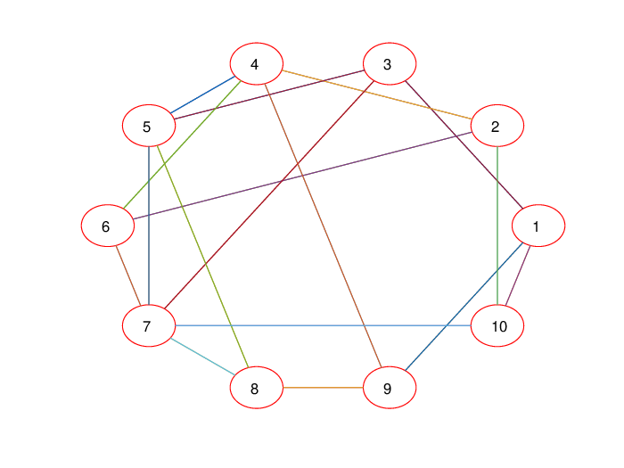
Example 1: In this example, Algorithm 1 is used to optimize the convergence rate on different graphs. Consider a third-order MAS with $10$ agents on four unweighted graphs: the graph $\mathcal{G}_{1}$ randomly generated by a small-world network model shown in Fig. 1, the cycle graph $\mathcal{G}_{2}$ , the path graph $\mathcal{G}_{3}$ , the complete bipartite graph $\mathcal{G}_{4}$ with $4+5$ vertices. Set $\tau=0.1$ , $T=5000$ , $\eta=0.01$ , and $\delta=10^{-6}$ . Randomly initialize the control gain $K^{(0)}$ multiple times, run Algorithm 1, and record the optimal convergence rate. The convergence rate $r^{*}$ obtained by Algorithm 1 is listed in Table I, where $r_{lb}$ represents the lower bound ${\left({\frac{{{\lambda_{N}}-{\lambda_{2}}}}{{{\lambda_{N}}+{\lambda_{2}}}}}\right)^{1/3}}$ . It can be found that on different graphs, the convergence rate $r^{*}$ of the third-order MAS can reach the lower bound $r_{lb}$ , and the smaller $\lambda_{N}/\lambda_{2}$ is, the smaller $r^{*}$ is. Next, generate the initial state of each agent in the interval $[-1,1]$ . The convergence of the consensus error ${\left\|{\bm{e}(k)}\right\|_{2}}$ on different graphs is shown in Fig. 2. It can be observed that the better the connectivity of the network is, the faster the consensus error converges.

Refer to caption — Fig. 1: The graph $\mathcal{G}_{1}$

TABLE I: Convergence rate on different graphs

	Graph $\mathcal{G}_{1}$	Graph $\mathcal{G}_{2}$	Graph $\mathcal{G}_{3}$	Graph $\mathcal{G}_{4}$
$\lambda_{N}/\lambda_{2}$	4.4790	10.4721	39.8635	2.5000
$r_{lb}$	0.8595	0.9381	0.9834	0.7539
$r^{*}$	0.8595	0.9381	0.9834	0.7539

Example 2: In this example, the effectiveness of the control strategy in Theorem 3 is verified. Consider the cycle graph $\mathcal{G}_{2}$ with $10$ nodes. The distinct non-zero eigenvalues of Laplacian matrix $\mathcal{L}_{\mathcal{G}_{2}}$ are $\{0.3820,1.3820,2.6180,3.6180,4\}$ . Let $\tau=0.1$ . Randomly set the initial state of the agents in the interval $[-5,5]$ . According to Theorem 3, when $n=2$ , consensus will be achieved at step $n\bar{l}=10$ as shown in Fig. 3, and the final consensus state of agent $i$ is $\bm{x}_{i}(k)=[1.3325+0.0963k,0.9627]^{T},k\geq 10.$ Similarly, when $n=3$ , consensus will be achieved at step $n\bar{l}=15$ as shown in Fig. 4, and the consensus state of agent $i$ is $\bm{x}_{i}(k)=[1.3325+0.0850k+0.0113k^{2},0.9627+0.2266k,2.2662]^{T},k\geq 15.$

VI Conclusions

The problem of accelerated asymptotic and finite-time consensus of discrete-time high-order MASs has been studied in this paper. Firstly, a protocol with constant control gains has been introduced to achieve consensus asymptotically. The fast consensus problem has been transformed into an optimization problem of convergence rate, and an accelerated consensus algorithm based on gradient descent has been designed to optimize the convergence rate. By using the Routh-Hurwitz stability criterion, the lower bound on the convergence rate has been derived, and the necessary condition to achieve this convergence rate has been proposed. Due to the limitation of constant control, consensus can’t be achieved in finite time. Hence, a protocol with time-varying control gains has been designed to achieve the finite-time consensus. Explicit formulas for the time-varying control gains and the final consensus state have been given. Numerical examples have demonstrated the validity and correctness of these results.

References

[1] Y. Cao, W. Yu, W. Ren, and G. Chen, “An overview of recent progress in the study of distributed multi-agent coordination,” IEEE Transactions on Industrial Informatics, vol. 9, no. 1, pp. 427–438, 2013.
[2] J. Qin, Q. Ma, Y. Shi, and L. Wang, “Recent advances in consensus of multi-agent systems: A brief survey,” IEEE Transactions on Industrial Electronics, vol. 64, no. 6, pp. 4972–4983, 2017.
[3] A. Dorri, S. S. Kanhere, and R. Jurdak, “Multi-agent systems: A survey,” IEEE Access, vol. 6, pp. 28 573–28 593, 2018.
[4] F. Chen, W. Ren et al., “On the control of multi-agent systems: A survey,” Foundations and Trends in Systems and Control, vol. 6, no. 4, pp. 339–499, 2019.
[5] L. Xiao and S. Boyd, “Fast linear iterations for distributed averaging,” Systems & Control Letters, vol. 53, no. 1, pp. 65–78, 2004.
[6] E. Kokiopoulou and P. Frossard, “Polynomial filtering for fast convergence in distributed consensus,” IEEE Transactions on Signal Processing, vol. 57, no. 1, pp. 342–354, 2009.
[7] S. Apers and A. Sarlette, “Accelerating consensus by spectral clustering and polynomial filters,” IEEE Transactions on Control of Network Systems, vol. 4, no. 3, pp. 544–554, 2017.
[8] E. Montijano, J. I. Montijano, and C. Sagues, “Chebyshev polynomials in distributed consensus applications,” IEEE Transactions on Signal Processing, vol. 61, no. 3, pp. 693–706, 2013.
[9] A. Y. Kibangou, “Step-size sequence design for finite-time average consensus in secure wireless sensor networks,” Systems & Control Letters, vol. 67, pp. 19–23, 2014.
[10] S. Safavi and U. A. Khan, “Revisiting finite-time distributed algorithms via successive nulling of eigenvalues,” IEEE Signal Processing Letters, vol. 22, no. 1, pp. 54–57, 2015.
[11] B. N. Oreshkin, M. J. Coates, and M. G. Rabbat, “Optimization and analysis of distributed averaging with short node memory,” IEEE Transactions on Signal Processing, vol. 58, no. 5, pp. 2850–2865, 2010.
[12] S. S. Kia, B. Van Scoy, J. Cortes, R. A. Freeman, K. M. Lynch, and S. Martinez, “Tutorial on dynamic average consensus: The problem, its applications, and the algorithms,” IEEE Control Systems Magazine, vol. 39, no. 3, pp. 40–72, 2019.
[13] G. Pasolini, D. Dardari, and M. Kieffer, “Exploiting the agent’s memory in asymptotic and finite-time consensus over multi-agent networks,” IEEE transactions on Signal and Information Processing over Networks, vol. 6, pp. 479–490, 2020.
[14] J.-W. Yi, L. Chai, and J. Zhang, “Average consensus by graph filtering: New approach, explicit convergence rate, and optimal design,” IEEE Transactions on Automatic Control, vol. 65, no. 1, pp. 191–206, 2020.
[15] J. Dai, J.-W. Yi, and L. Chai, “Optimal memory scheme for accelerated consensus over multi-agent networks,” IEEE Transactions on Signal and Information Processing over Networks, vol. 8, pp. 344–352, 2022.
[16] W. He and J. Cao, “Consensus control for high-order multi-agent systems,” IET Control Theory and Applications, vol. 5, no. 1, pp. 231–238, 2011.
[17] Q. Zhang, Y. Niu, L. Wang, L. Shen, and H. Zhu, “Average consensus seeking of high-order continuous-time multi-agent systems with multiple time-varying communication delays,” International Journal of Control Automation and Systems, vol. 9, no. 6, pp. 1209–1218, 2011.
[18] W. Yu, G. Chen, W. Ren, J. Kurths, and W. Zheng, “Distributed higher order consensus protocols in multiagent dynamical systems,” IEEE Transactions on Circuits and Systems I, vol. 58, no. 8, pp. 1924–1932, 2011.
[19] H. Rezaee and F. Abdollahi, “Average consensus over high-order multiagent systems,” IEEE Transactions on Automatic Control, vol. 60, no. 11, pp. 3047–3052, 2015.
[20] A. Abdessameud and A. Tayebi, “Distributed consensus algorithms for a class of high-order multi-agent systems on directed graphs,” IEEE Transactions on Automatic Control, vol. 63, no. 10, pp. 3464–3470, 2018.
[21] S. Li, H. Du, and X. Lin, “Finite-time consensus algorithm for multi-agent systems with double-integrator dynamics,” Automatica, vol. 47, no. 8, pp. 1706–1712, 2011.
[22] K. You and L. Xie, “Network topology and communication data rate for consensusability of discrete-time multi-agent systems,” IEEE Transactions on Automatic Control, vol. 56, no. 10, pp. 2262–2275, 2011.
[23] A. Eichler and H. Werner, “Closed-form solution for optimal convergence speed of multi-agent systems with discrete-time double-integrator dynamics for fixed weight ratios,” Systems and Control Letters, vol. 71, pp. 7–13, 2014.
[24] G. Parlangeli and M. E. Valcher, “Accelerating consensus in high-order leader-follower networks,” IEEE Control Systems Letters, vol. 2, no. 3, pp. 381–386, 2018.
[25] R. Olfati-Saber and R. M. Murray, “Consensus problems in networks of agents with switching topology and time-delays,” IEEE Transactions on Automatic Control, vol. 49, no. 9, pp. 1520–1533, 2004.
[26] C. Ma and J. Zhang, “Necessary and sufficient conditions for consensusability of linear multi-agent systems,” IEEE Transactions on Automatic Control, vol. 55, no. 5, pp. 1263–1268, 2010.
[27] L. Li, M. Fu, H. Zhang, and R. Lu, “Consensus control for a network of high order continuous-time agents with communication delays,” Automatica, vol. 89, pp. 144–150, 2018.
[28] S. Boyd and L. Vandenberghe, Convex optimization. Cambridge university press, 2004.
[29] T. Chang and C. Chen, “On the routh-hurwitz criterion,” IEEE Transactions on Automatic Control, vol. 19, no. 3, pp. 250–251, 1974.
[30] B. Mertzios and M. Christodoulou, “On the generalized cayley-hamilton theorem,” IEEE Transactions on Automatic Control, vol. 31, no. 2, pp. 156–157, 1986.