Genomic Compression with Read Alignment at the Decoder
Abstract
We propose a new compression scheme for genomic data given as sequence fragments called reads. The scheme uses a reference genome at the decoder side only, freeing the encoder from the burdens of storing references and performing computationally costly alignment operations. The main ingredient of the scheme is a multi-layer code construction, delivering to the decoder sufficient information to align the reads, correct their differences from the reference, validate their reconstruction, and correct reconstruction errors. The core of the method is the well-known concept of distributed source coding with decoder side information, fortified by a generalized-concatenation code construction enabling efficient embedding of all the information needed for reliable reconstruction. We first present the scheme for the case of substitution errors only between the reads and the reference, and then extend it to support reads with a single deletion and multiple substitutions. A central tool in this extension is a new distance metric that is shown analytically to improve alignment performance over existing distance metrics.
Index Terms:
Distributed Source Coding, Generalized Concatenation, Coset Coding, Genomic Sequencing Data, Alignment.I Introduction
Genomic sequencing is the process of analyzing the order of nucleic acids within a DNA molecule (genomic sequence). In many modern sequencing technologies, a large set of short sequence fragments, called reads, is produced and represented by a string of characters (usually A,C,G,T). In this method, called shotgun sequencing [1], each read’s location within the sequence is generally unknown. Furthermore, the sequencing machine introduces mutation errors into the reads. Therefore, the sequence assembly from the reads requires a large number of reads and high computational effort. Effective compression of pre-assembly reads data is therefore an essential problem. A large number of read-compression methods are available [2, 3, 4], partitioned into two main categories: reference-free and reference-based tools, differing by whether a closely similar reference genome is shared by the encoder and decoder. In some applications, genome reads will be produced at an edge node, e.g. a physician’s office, and then sent for processing to a central node, e.g. a cloud database. In such scenarios, the cost of known reference-based and reference-free methods may be too high for the edge node’s limited resources, due to the need to store long references and perform costly alignment (in the former), and cluster reads and use powerful compressors (in the latter). Alternatively, in this paper we propose a compression scheme in which the encoder needs to neither store references nor perform heavy processing, while benefiting from a reference available at the central node decoding the reads.
Compression with a reference, acting as side information available only at the decoder, is an instance of the well known Slepian-Wolf (SW) coding problem [5]. This source coding problem was first described as an equivalent channel coding problem over a virtual difference channel between the sources by Wyner [6], and an explicit construction based on the syndromes of error-correcting codes was first introduced in the pioneering work of Pradhan and Ramchandran [7]. Several works offered improved constructions and/or analysis approaches [8, 9, 10, 11, 12, 13]. Some works even dealt specifically with genomic data [14, 15], but focused on either full-block or streamlined data, and not fragmented reads from randomly chosen and unknown locations. When compressing fragmented reads, the known capability of reconstructing a read from a similar reference is not sufficient, and additional information is needed for aligning the read within the full reference.
In this work, our objective is to compress a batch of reads taken from a long genome sequence, such that a decoder with a reference similar to this genome can perfectly reconstruct all the reads without error. The construction proposed in Section III of this paper offers both alignment and reconstruction capabilities, using the framework of generalized error-locating (GEL) [16] coset codes. GEL coset codes were used in the Cassuto-Ziv construction [13] for full-block compression, and the novelty of this present work is in using the GEL’s hierarchy of inner codes to combine all the information for read reconstruction into the same codeword: one layer for alignment, one for similarity reconstruction and one for reconstruction validation. In the fourth layer, a batch of reads is encoded with an outer code to provide extremely low failure probability. We begin by assuming that the errors between the sequence, its reads and the reference are modeled by substitution errors alone, and propose an efficient coding scheme for such a scenario. The construction uses general linear codes, and in addition we show how to specialize it using known algebraic codes such as BCH codes.
We continue by extending the scheme to deal with a single deletion introduced to a read in addition to the substitution errors. This model is justified by substitution errors being the dominant error type in many sequencing technologies, while having some deletion errors that are more rare. Toward that extension, we propose in Section IV a new efficiently computable distance measure, called shift-compensating distance, that is analytically shown to reduce the false-alignment probability significantly compared to a commonly-used distance measure. Then, in Section V, we modify our coding scheme to support these deletion errors. In Section VI, we pursue the probabilistic analysis of the scheme. These results are used as a design tool for setting the scheme’s parameters for compression rate minimization, while meeting a given specification of perfect read-recovery success probability. Finally, in Section VII we suggest further extensions, and in Section VIII we colnclude and suggest topics for future work.


II Problem Formulation
II-A Problem Setting
A genome data being sequenced in an edge node is represented by a string , for some alphabet of size . A closely similar reference of this data, represented by , is stored in a central node, and is unavailable at the edge node. The differences between and are assumed to be caused by genetic diversity [17]. A sequencing machine at the edge node generates a batch of reads from , denoted by . Each read is an approximate sub-sequence of , taken from an unknown random location within , and introduced with sequencing errors. Our goal is to encode the reads to a minimal size, such that they can be perfectly recovered from the similar reference . The encoder output is communicated to the central node without errors.
II-B Substitutions Channel Model
We begin by modeling errors using a substitutions-only channel; later in the paper we also address deletion errors. The genetic diversity is modeled as , a -ary symmetric channel for which
We now let be a sub-sequence observed by the sequencer, where is a random, unknown starting index. A read with sequencing errors is modeled by a similar -ary symmetric channel: . We call the sub-sequence of with proper alignment to the read .
Lemma 1
. Let . Then for a proper alignment we have .
Proof:
It follows that
∎
The relations between the genome, reference and reads are illustrated in Fig. 1 (left).
Remark: Although in the statistical model in Lemma 1 we define as the channel input, one should notice that in the operational problem we need to reconstruct from , and not the other way around as in standard channel coding.
The induced equivalent channel serves as the difference channel between the side information (reference segment) and the source (corresponding read), for which an error-correcting code should be designed [6, 7]. In our coding scheme, we will add a layer enabling the alignment of each read to the reference in order to find a closely matching segment to reconstruct from. A modification of the scheme to deal with a channel model including a single deletion per read in addition to the substitution errors is developed in Sections IV,V. We choose in this paper the channel model with a single parameter for simplicity, while in future work one may consider richer models (e.g. [18]), potentially exploiting the dependence between two overlapping reads, whose references pass through the same instantiation of the channel .
II-C Pre-Decoding Alignment
We wish to encode such that only the information required to reconstruct it from is transmitted. Nevertheless, the decoder first needs to know the starting index . Therefore, the encoder must transmit some additional information enabling the decoder to align the read within the reference, while accounting for the substitution errors. This alignment information is an -bit function called read identifier. The value of is set as a tradeoff between alignment quality and compression rate. Since only partial information is provided for alignment, additional improper alignments, i.e., erroneous starting indices, are likely to be found. The alignment process provides the decoder with a set of length- segments of as candidates for read reconstruction. Every can be regarded as a sequence from which is obtained by passing through a useless channel with zero mutual information. The alignment process is illustrated in Fig. 1 (right). Clearly, only the proper alignment is desired for decoding, thus a method for rejecting improper candidates is required. This method, described in Section III, is referred to as validation.
III The Compression Scheme
For simplicity, from this point on we assume , i.e. , but every result can be generalized to any that is a prime power. Furthermore, cyclic 1-based indices will be used, i.e., every index in will be taken as to avoid edge effects and for the ease of notation.
III-A Read Identifier
A simple bit sampling approach is found to be very suitable for read identifiers. Let be a predefined set of indices, known to both the encoder and decoder. Now, let be the read identifier. In this case, an aligner at the central node simply correlates this identifier along the reference using the Hamming distance with respect to each starting index, and produces the set
| (1) |
where is the Hamming distance, is a predefined threshold, and
is the set of matching alignments of within . The remainder of the read, i.e., the indices outside of the identifier, is denoted by , where . In Section V-C we will show that taking evenly spaced over the read is preferable over a simple prefix when the model includes deletion differences.
III-B General Code Construction
We wish to encode and transmit a batch of reads from such that a decoder with access to satisfying will perfectly reconstruct them with high probability. Recall from Section II-B that is the equivalent error probability between a proper alignment in to its corresponding read .
Definition 2
. A -code is a pair of encoder-decoder for a set of length- reads such that:
- 1.
has access only to ,
- 2.
has access only to and ,
- 3.
the encoded size satisfies ,
- 4.
the correct-decoding probability satisfies
is a decoding success probability requirement specified for the coding scheme, and is its (fixed) compression rate. Our general code construction is based on generalized error locating (GEL) codes [16], and specifically on the Cassuto-Ziv code construction [13], adapted to use as a source code with alignment-validation capabilities.
Construction 1. Let be a pair of binary linear codes with parameters , where . Let be parity-check matrices of these codes, respectively, such that is obtained from by concatenating a validation matrix of rows that are linearly independent of the rows of . Let be a complementary matrix such that concatenating it with forms a square full-rank matrix . This structure is illustrated in Fig. 2.

Finally, let be a linear, maximum-distance separable (MDS) [19] outer code over , with parity-check matrix , where .
The encoding process is given formally in Algorithm 1, and we now describe its main steps in words. For every read , we first extract its read identifier , and then for the remaining indices we calculate the syndromes with respect to , respectively. This process is referred to as the inner encoding. The syndromes are regarded as elements in and collected to a word , and the syndrome of with respect to is calculated. This is referred to as the outer encoding. The encoder outputs the read identifiers , the inner syndromes , and the outer syndrome . We note that the inner syndrome can be described as , where correspond to , respectively.
for do // Inner Encoding
Calculate ,
Form
Calculate // Outer Encoding
Output:
The decoder for the construction is presented formally in Algorithm 2, now also explained in words. Each read identifier is first aligned over to form from (1). We set a flag ‘found’ to , and then for every candidate we extract , and decode it with the function that finds the nearest word to with syndrome with respect to . The result of each decoding is validated by computing its syndrome with respect to , and comparing it to the received . If equal, and the flag ‘found’ is (meaning it is the first candidate to pass validation), we calculate the estimated outer syndrome of with respect to , and update the flag ‘found’ to 1. If some passes validation when ‘found’ is set to 1 (meaning it is not the first to pass validation), we set the estimated outer syndrome to an erasure, i.e, . Furthermore, if all decoding outputs fail validation, an erasure is also set to . This process, referred to as the inner decoding, is repeated for every read . Then, outer decoding is performed by decoding the word of estimated outer syndromes , over , with respect to within the coset of syndrome , to form . Finally, the syndrome of each with respect to the full-rank is estimated by concatenating sent by the encoder and resulted from outer decoding, and is then mapped to the single word of this syndrome with respect to . The estimated read is finally reconstructed by inserting the read identifier sent by the encoder to the suitable indices.
The inner-decoder finds the minimal-weight error word for which , and outputs . This function can be easily implemented using standard syndrome-based decoders that do the same, only for the special case . In this paper we assume that is a bounded-distance decoder [20], discarding error words with distance higher than half the code’s minimum distance. Similarly, , decodes with respect to to a syndrome . denotes the linear mapping of to the word of syndrome with respect to .
We also note that the validation process includes cases of misvalidation, that is, a vector passing validation, not to be confused with the case of a failed validation, happening when , which forms a rejection of the candidate.
for do
Calculate
if then // Validation
else // More Than One Candidate
Decode , where
for do // Inverse Mapping
Reconstruct from Output:
Proposition 3
. The rate of Construction III-B is given by
Proof:
Every contain bits, respectively. contains elements, each represented by bits. Hence,
Dividing by information bits completes the proof. ∎
Proposition 4
. Construction III-B yields an -code if and only if at the outer-decoder output .
Proof:
By the definition of , we have if and only if their syndromes with respect to are identical. Furthermore, since is known to the decoder, the former implies . Since is also known to the decoder, if , the decoder has the correct syndrome bits with respect to , and can recover perfectly. ∎
The design of the scheme’s parameters for minimization of the compression rate is pursued in Section VI.
III-C Employing Algebraic Codes in the Construction
Toward practically realizing the coding scheme, in this sub-section we study the use of known algebraic codes, with emphasis on adapting their use to source coding, and in particular to the requirements of Construction III-B. Specifically, as the inner codes we will use the well-known binary primitive BCH codes [19]. For the outer code, we will use the also very well-known Reed-Solomon (RS) codes, which enjoy the desirable MDS (maximum distance separability) property. Both these code families have known efficient algebraic decoders (e.g., the Berlekamp-Massey algorithm [21]), capable of correcting both errors and erasures [22].
The main challenge of using BCH codes is that their canonical representation is not as binary parity-check matrices (as in Construction III-B), but rather given over a finite field , where is an integer that for code-length satisfies . To guarantee the requirements of Construction III-B, we will focus on obtaining the following properties using BCH codes: (i) constructing a pair of codes whose syndromes are nested, (ii) implementing the inner decoder using existing algebraic BCH decoders, and (iii) finding a complementary matrix ensuring of full rank, preferably one offering efficient realization of the inverse mapping .
For , let be a binary BCH code that can correct up to errors, such that . Property (iii) above can readily be obtained by a systematic representation of the code , a fact we show later in the section. However, a systematic parity-check matrix of a BCH code in general does not contain the rows of a systematic parity-check matrix for the BCH code , which challenges Property (i). Furthermore, Property (ii) requires computation of algebraic syndromes (to be discussed later), which are different from the binary syndromes computed in Algorithm 1 and supplied to the decoder.
To solve this, we will show that one can choose arbitrary systematic parity-check matrices for and in the encoder, and still be able to use standard syndrome-based algebraic BCH decoders. To do this, we exploit a type of nesting that BCH codes do have: with respect to their algebraic syndromes over . Let be a length- binary word. Its algebraic syndrome is defined as follows [19].
Definition 5
. For every , let . Let be a primitive element of . Then, the -correcting algebraic syndrome of is defined by
Note that the algebraic syndrome is a vector of length over . For , denote by the algebraic syndrome of with respect to . Similarly, denote by the binary syndrome of with respect to , computed by a systematic parity-check matrix . By the definition of the BCH construction, we have the following.
Observation 6
.(Nested syndromes) Let be the algebraic syndromes of with respect to respectively. Then, the first elements of are equal to .
The following lemma shows that the algebraic syndrome of can be recovered from its binary syndrome.
Lemma 7
. Let be a parity-check matrix of having the identity matrix in its last columns. If , then it follows that , where of length .
Proof:
Let us look at the following parity-check matrix
where the elements are taken as binary column vectors of length . It is known that this matrix defines the binary BCH code , albeit not in a systematic form [19]. Therefore, and span the same linear space, implying there is a linear-transformation matrix such that . Now, by the systematic form of , it is clear that . Hence, we get
| (2) |
Finally, it can be seen that the structure of is directly related to the algebraic syndrome, as we can write
in which the -th row exactly correspond to the -th element of the algebraic syndrome, meaning (in binary representation). Combining with Equation (2), we get , completing the proof. ∎
Now, let (possibly a shortened version of a primitive BCH code). When for we use a systematic parity-check matrix (whose last columns form an identity matrix), for the complementary matrix we can use , where denotes the identity matrix, and 0 denotes an all-zeros matrix of size . The vertical concatenation of and is full rank, because both matrices are full rank, and given their structure no linear combination of rows of can give a row of (and vice-versa). Furthermore, by using this matrix, the calculation of the syndrome turns out to be simply extracting the first bits of .
Realizing Construction III-B with BCH and RS codes
Based on the discussion above, we can now introduce the realization of the construction using algebraic codes. Let , where denotes a Reed-Solomon code. This code is taken over , with , by dividing the bits computed by into sections, and encoding each section separately into a codeword. By keeping small enough (e.g. ), the field’s order remains practical for processing regardless of the inner code’s dimension.
The encoder remains almost identical to Algorithm 1, with the following specifications:
- •
(the binary syndrome) is computed with a systematic for ,
- •
is taken as the first bits of ,
- •
is computed as a concatenation of algebraic syndromes of .
The decoder is realized based on the following modifications to Algorithm 2:
- •
Calculate (the algebraic syndrome), and extract as the first elements of it.
- •
Using an algebraic BCH decoder, decode within the coset of the syndrome .
- •
Compute the algebraic syndrome of the decoded word, , and compare its last elements to the corresponding elements in for validation.
- •
The mapping is realized by encoding to a codeword whose first bits equal (that can be easily done using ), and then setting . The correctness of this step follows by the structures of , discussed above.
IV A Distance for Alignment with Deletions
To extend the coding scheme to also deal with deletion errors, we need to establish an efficient way to perform alignment (at the decoder) under such errors. With substitutions only, an alignment candidate is considered suitable if its Hamming distance to the read is small (see (1)). We now need an alternative distance measure that supports deletion errors between the reference and the sequenced reads. Ultimately, the distance measure proposed in this section will be used in the next section (Definition 17) to replace the alignment condition (1). We focus on the case of a single deletion (and multiple substitutions) per inner block, and discuss extensions to multiple deletions (and to insertions) toward the end of the paper. Note that we can partition any read of given length into multiple inner blocks of any desired size, and therefore by keeping the inner-blocks short, a single deletion remains an interesting case in practice for a wide range of deletion probabilities.
IV-A Existing Measures
An immediate candidate for such a measure is the Levenshtein distance [23], counting the minimal number of edits (deletions, insertions and substitutions) required to obtain one word from another. Nevertheless, this measure suffers from two main issues in our case: (i.) its complex calculation by dynamic-programming algorithms makes it impractical to evaluate each read along every possible offset in the reference, (ii.) allowing unrestricted error patterns, involving any combination of edits, introduces unfitting alignment candidates.
Another possible measure is the shifted Hamming distance [24], which matches each read index with adjacent indices in the sub-sequence considered for alignment. For our purposes, since only deletions (and not insertions) are considered, it is sufficient to use shifts in one direction between the two input sub-sequences. This can be formalized by
| (3) |
where denotes a logical ‘AND’ operation, and denotes a word of length from alphabet , and the binary operator returns for equal symbols and otherwise. The main issue with this measure is that it allows low distance values from independent shifts between indices, ignoring the special shift structure of index deletion. This causes even random unrelated sequences to be declared close, increasing the number of improper alignments.
IV-B Preliminaries
The following definitions are the basic building blocks for our proposed distance measure.
Definition 8
. (Cumulative Hamming distance) For , , define, for every and every ,
where denotes an addition over . When clear from the context, we will denote .
Definition 9
. Let , . Define, for every and every ,
where by definition . Again, when clear from the context, we will denote .
IV-C Single-Deletion Shift-Compensating Distance
We can now introduce the desired distance measure. Intuitively, it measures the Hamming distance between two words, while compensating for a possible block shift caused by a single deletion occurring in one of them before entering the substitution channel.
Definition 10
. Let , and let
| (4) |
Then, we define the shift-compensating distance by
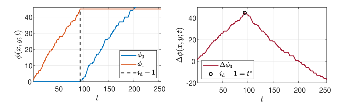
Note that , because is non-decreasing and is non-negative. Let us give some intuition to this measure through a simplified example. Let be the word obtained from by a deletion occurring in position . Then, for every , and for every . Therefore and . It follows that , and so it is clear that (otherwise implying a negative ). We conclude that: (i) an index maximizing gives an estimate for the deletion location (up to an ambiguity within a run of the same symbol around the deletion), and (ii) after estimating the deletion location, gives the combined Hamming distance before and after this estimated location, while shifting the second part of to compensate for the deletion. These conclusions are illustrated in Fig. 3, where in the right plot it is evident that , thus locating the likely deletion position. The shift compensating measure sums the increments of (blue) left from and the increments of (red) right from , which sum to zero since there are no substitutions. When introducing substitutions, these horizontal segments in will include random increases, with an average slope of , attributed to the substitutions.
IV-D Similarity Properties
In this sub-section we formalize the properties of . First, we examine its relation to the underlying Hamming distance.
Lemma 11
. Let . Let denote the word obtained from by a deletion in index , for any . Then,
| (5) | |||
| (6) |
Proof:
It holds that
Minimizing over we get by definition, and the minimizing argument is exactly . ∎
It is seen in (5) that is the most natural distance for this error model: it gives the minimal Hamming distance between and any single-deletion version of . Importantly, it has a linear calculation complexity making it more practical than other alternatives, such as the Levenshtein distance.
Next, to analyze the new measure’s alignment performance, in particular its ability to reject false alignment positions (thus reducing the count of improper alignments), we study its distribution when evaluated on a random word unrelated to . We first observe that for two independent random words , we can write , where , and are independent random variables with support and probabilities , respectively. This type of sum forms a symmetric random walk with null steps. Furthermore, we observe that in this case is a Binomial random variable with . Based on these observations, we get the following theorem.
Theorem 12
. Let us denote by the random variable of for randomly chosen . Then,
where we defined
for , and , the multinomial coefficient.
Proof:
The full formal proof is given in Appendix C. We include a sketch here. To count the number of sequence pairs that have , we classify the pairs according to several variables appearing as summation indices. The primary variables are that is the value calculated in (4), and that is . Given , we count the number of random walks of that attain a global maximum of at time , and for each such walk expand the number of sequence pairs that have distance . The variables and count the number of zeros of the random walk in total and until time , respectively. The remaining summation indices are weight variables: for the sub-sequence until time , and for the sub-sequence thereafter. ∎
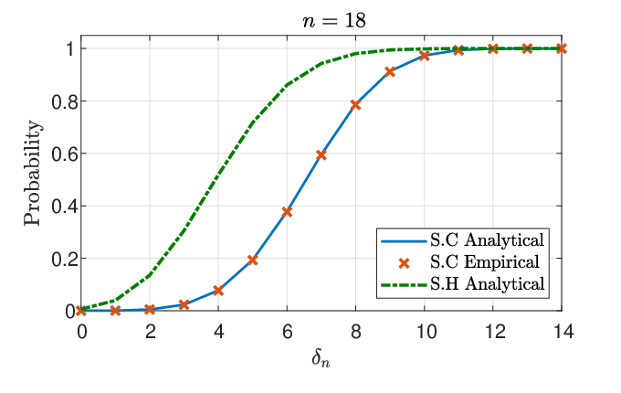
We plot in Fig. 4 the distribution (CDF) of for obtained by Theorem 12 (solid). To validate the theoretical result, we include in the plot the empirical distribution collected from random sequences (red croses). We also show, in comparison, the CDF of the shifted-Hamming distance given in (3) (dashed green), demonstrating the significant advantage of in obtaining high values for unrelated sequences.
IV-E Metric-Like Properties
In this section we show that our distance meets most of the conditions for being a metric. More specifically, we define a semi-metric, which has all the properties of a standard metric [25], short of a single technical property, and prove that our distance meets this definition.
Let us denote , that is the set of all words with entries from and lengths satisfying .
Definition 13
. (Multi-length semi-metric) For every , the function is called an -length semi-metric if it satisfies:
- 1.
(symmetry).
- 2.
such that or , it follows that (triangle inequality).
- 3.
Let . Then for every we have , as some deterministic set depending only on and the word , such that (generalized identity of indiscernibles).
These properties are similar to the properties defining a standard metric, with a generalization of the known identity of indiscernibles [26], which will be useful as described after Proposition 15.
We now use to form a natural symmetric distance, which is proved to be such a semi metric.
Definition 14
. Let . The symmetric shift-compensating distance is defined by
Proposition 15
. The distance is an -length semi-metric for any .
Proof:
We follow the conditions in Definition 13. We denote by the deletion and insertion balls of radius 1 of , respectively.
- 1.
The symmetry is immediate from the definition.
- 2.
For the Hamming distance, the triangle inequality holds. For we examine two cases: (i.) Let be some word such that , then
where is the minimizing index, and so
(ii.) Let be some word such that . Similar to the former case . Furthermore, for every we have , since an index is discarded in summation. Therefore,
For and ,
Hence, , the triangle inequality holds.
- 3.
Based on Hamming distance properties we have . For some , based on Lemma 11, we have if and only if , i.e. . Since the latter occurs if and only if , we get .
∎The generalized identity of indiscernibles with captures well the fact that multiple length- sequences are 1 deletion and 0 substitutions away from a length- alignment target , having distance as itself.
V Extending The Scheme to Single-Deletion Multiple-Substitutions
V-A Channel Model
In this section we extend the difference channel model to single-deletion multiple-substitutions (SDMS) in each read.
That is, for each read there exists an index such that the read is obtained from , of length , by a single deletion and a certain number of substitutions. Equivalently, there is an integer such that
where is the result of passing through a substitution channel. In this model we have: (i) the -th index with respect to the segment, i.e. the with respect to the sequence, is deleted, and (ii) the last symbol in , i.e. is observed, keeping the length of the sequencer’s output as . This error model represents two equivalent scenarios: (i) the sequencer ‘skips’ a symbol, while unknowingly keeping on sequencing an extra symbol to keep the length as defined, and (ii) the reference includes an insertion with respect to the sequenced genome due to genomic diversity. These result in the same relation between and , and in both the sequencer is unaware whether a deletion occurred or not.
V-B Alignment with Single-Deletion
A modification to the pre-decoding alignment described in Section II-C is required in order to deal with a potential deletion error in every read. This is done by simply replacing the Hamming distance with the proposed shift-compensating distance. To deal with the non-consecutive read identifier used for alignment, the calculation of is easily extended to non-consecutive indices by
where consecutive index shifts (not restricted to the subset of indices sent to the decoder) are used only in , thus are available to the decoder. Denoting , is now the corresponding modification of Definition 10:
| (7) |
We now show an important property similar to Lemma 11, showing that captures the read identifiers’ Hamming distance to the closest single-deletion vector.
Lemma 16
. Let be the word obtained from by a deletion in index , and let be an arbitrary word. Then,
| (8) |
Proof:
We have
Since is obtained by the minimization of this expression with respect to , we get
where is the unique index such that . From this the statement follows. ∎
Definition 17
. Let , and let be taken from some offset in . We say that matches if , for some integer distance threshold .
Now, by aligning the read identifier to , each such match yields a length- candidate , and all matches form the set . This view readily captures reads without deletions, which can be modeled as deleting the -th index of .
V-C Generating Sub-Candidates for Each Alignment Candidate
In contrast with the substitutions-only case, we now need to account for a deletion in before decoding. Toward that, the extended scheme generates a list of sub-candidates , according to the following procedure. Define to be a global integer tolerance parameter, and denote by the value of that minimized in (7) to obtain . We denote here , and . Then the set is defined by all deletion indices that satisfy the following:
| (9) |
that is, all deletion-indices within intervals of the read identifier’s indices around , with exceptions at the extremal indices. For , i.e., no tolerance, we have , whereas for we have , i.e., , where denotes the single-deletion ball. It is motivated to use because due to substitutions, the true deletion index in may fall outside its estimated interval defined by . The value of controls the number of vectors qualifying to reconstruct by inner decoding, and it may be set to best balance successful reconstruction from the proper alignments with effective rejection of false candidates. It can now be seen that by taking evenly spaced , undesirable large intervals can be avoided.
V-D Inner-code Decoding with Multiple Sub-Candidates
Recall from Section III-B that in the substitutions-only case each candidate is passed to inner-code decoding and validation. Now with deletions, we need to decode and validate a set of sub-candidates . To see how this should be done, we note the following observation.
Observation 18
. Let , and let . Then, for ,
This means that if is the actual deletion index and is the one chosen for some sub-candidate, this mismatch may introduce errors only in the region between those two indices, defined as the error region, as illustrated in Fig. 5.

It is thus likely that for the proper alignment of , multiple sub-candidates with deletion indices close to will correctly decode to , even if contains some substitutions with respect to . This motivates the following treatment of in the modified decoder, specified in Algorithm 3. For every candidate : (i.) Decode and validate every sub-candidate , (ii.) store any that was successfully decoded and validated, and the number of its appearances along the decoding instances in , (iii.) apply a majority rule
| (10) |
From this point, takes the role of as defined in the decoding of Construction III-B, and the rest of the decoding process is unaltered. The encoding process is also unchanged.
for do
Set
for do // Inner Decoding
for every do
Calculate
if then // Validation
Set
else // More Than One Candidate
Decode , where
for do // Inverse Mapping
Reconstruct from Output:
VI Probabilistic Analysis for Setting Code Parameters
In this section we analyze the compression scheme proposed in Section III when used with -correcting inner codes and MDS outer codes. The main purpose of this analysis is to serve tools that can help in setting the code and alignment parameters. Since the compression rate of the scheme is fixed by the code parameters, we focus on analyzing the probability that the block of reads is successfully reconstructed by the decoder with no error. Throughout this section, we model the genome as an i.i.d. Bernoulli sequence, and in addition assume the relation (Lemma 1) for the proper alignment. Extension of the analysis to other genome statistical models can be done based on related studies such as [1, 27].
We begin our anaylsis for the case of substitution-errors only, and extend it to the case of SDMS errors in Sections VI-C and VI-D. The analysis has two main components: first analyzing the inner-code performance as a function of the alignment parameters and the inner-code parameters, and then the outer-code performance as a function of the inner-code performance and the outer-code parameters. The outer-code analysis is the same for both error models.
For the analysis, we denote by , , the probability mass function (PMF) and cumulative distribution function (CDF) of a binomial random variable with parameters , evaluated at the value of , respectively. We also denote as the volume of a Hamming ball with radius of length- words. Finally, we denote .
VI-A Inner-Code Analysis
The inner decoder is invoked in Algorithm 2 on both the proper alignment of in (if found), denoted by , and, possibly, on improperly aligned vectors that are not related to . The scheme’s performance depends on the inner-decoding outcomes for both types of inputs. We begin with the proper alignment.
Definition 19
. The following probabilities are defined:
- •
- for succeeding in both alignment and decoding, i.e., and ,
- •
- for succeeding in alignment and misvalidating the reconstruction, i.e., , and ,
- •
- for failing in either alignment or validation, i.e., or .
As seen above, we use the superscript to represent probabilities pertaining to the proper alignment. The probabilities in Definition 19 describe every possible outcome of the proper-alignment inner decoding, hence . Therefore, it suffices to evaluate and .
Lemma 20
. Let . Then we have
Proof:
The first term is the probability of not exceeding the threshold of substitutions in the read identifier. The second term is the probability of not exceeding the substitution-correction capability of in the inner decoding. Since the indices of alignment and inner decoding are disjoint, the events and are independent, and we get a multiplicative joint probability. ∎
For the calculation of , we detail the properties of decoding and validating within specific code cosets.
Definition 21
. Let be a linear code with a parity-check matrix . Then, let be the coset of the code with syndrome , given formally by
where is a minimal-weight word such that .
We use the following well-known lemma, which we include with proof due to our non-standard notation.
Lemma 22
. Let be a syndrome of with corresponding to , respectively. Then .
Proof:
By the nested structure it is known that , and for every such that , we get . Since , we get , therefore and can be written as , where . Hence, for any word , we have that , where . By the latter, we get . ∎
We now analyze the probability of misvalidating a random word, which will be used in an upper bound for .
Definition 23
. Let with , and let be a random word chosen uniformly from the entire space . Then the probability of misvalidating , denoted , is the probability of miscorrecting with the decoder of to some , such that .
Lemma 24
. The probability of misvalidating a random word satisfies
| (11) |
Proof:
Let , and let be a random word. Then, by Definition 23, the misvalidation probability is the probability of being decoded (miscorrected) by the bounded-distance decoder of to a word within . Formally, define the set
| (12) |
for which the condition for misvalidation is: . The size of this set is , because the balls of radius do not intersect, and the misvalidation probability is thus
∎
For the following, we assume that is a proper code [28], a definition that covers any code whose probability of undetected error (miscorrection) is monotonically increasing with the substitution probability of the channel. This restriction is only for simplifying the probability expressions, and it is in no way necessary for practically reaching performance targets using the subsequent analysis. Moreover, many codes are proper for most of the distance range (e.g. BCH [29], LDPC [30]). We can now complete the analysis of the proper alignment.
Lemma 25
. The probability of misvalidating the proper alignment satisfies
| (13) |
Proof:
The first term is again the probability of successful alignment. Due to the properness of , for every , the probability of miscorrecting the noisy read, i.e., having it fall within a Hamming ball of radius centered on some codeword of , is upper bounded by the probability of miscorrecting a random word. ∎
Now, we move to analyze improper alignments, and our main objective is upper bounding the probability that one or more improper alignments will be misvalidated, an event that induces either an erasure or an error in the outer codeword.
We denote by the probability of having at least one misvalidated improper alignment (accepted at alignment as candidate, and then miscorrected and validated).
Lemma 26
. It holds that
Proof:
Let denote a read corresponding to some starting index , and aligned over the reference . Let denote the indicator of the event in which is improperly aligned, and misvalidated with respect to , for any . Then,
where the inequality is due to the union bound [31]. Note that the probability is conditioned on the fact that , for some (the proper alignment). We keep this conditioning implicit, but take it into account in the derivation of . Assume without loss of generality that (the other direction follows similarly from symmetry), and denote . If (no overlap), the conditioning can be ignored because on disjoint indices and are independent Bernoulli vectors. Thus we get
| (14) |
where the independence between alignment and misvalidation follows from their disjoint indices. In the case we need to be more careful, because due to overlap the vectors and are no longer independent. Denote , . We now prove that is uniformly distributed on the set when the sequence is drawn i.i.d. Bernoulli, as assumed in the model. To do this, we fix an arbitrary , and calculate the probability that , where subtraction is bitwise modulo .
From the uniform distribution of , we can rewrite the same probability as
It can be observed that when fixing the subsequence , the indicator function is evaluated to for exactly one sequence that satisfies all the constraints in the argument (left-hand side values up to are set by and , and from onward they are set by the previously set values and ). When summing over all assignments to , we get
proving the uniform distribution of .
The uniform distribution of the difference between and implies that the validation outcome of is independent from the fact that (with syndrome ) is likely proximate to . We can thus invoke Lemma 24, and get
| (15) |
where in this case we upper bound the alignment-success probability by , due to possible dependence between overlapping identifier bits when conditioning on the proper alignment. Since there are indices with , and indices for which , we get the desired upper bound. ∎
VI-B Outer-Code Analysis
In the outer code, the syndromes with respect to are treated as symbols in , which may be erased depending on the outcome of the inner decoding. Furthermore, a misvalidated inner-decoder output may introduce an erroneous symbol. The outer-decoded word can thus be modeled as transmitting through an outer channel introducing erasures and errors. The probabilities of these events are directly induced by the probabilities of the inner-decoder outcomes, analyzed in the previous sub-section. We can now examine the erasure and error probabilities of the outer channel, denoted by , respectively.
Lemma 27
. The following upper bounds hold
Proof:
An erasure occurs if there are no validated candidates (i.e., the proper alignment fails and no improper alignment is misvalidated), or more than one candidate has been validated. Hence,
An error occurs if the proper alignment is misvalidated and no improper alignment is misvalidated, or the proper alignment fails and exactly one improper alignment is misvalidated. The probability of exactly one improper misvalidation is upper bounded by . Hence,
∎
To obtain explicit upper bounds for , we substitute into the inequalities of Lemma 27 the corresponding values from Lemmas 20, 25, and 26, together with the relation . We can now derive the redundancy of the outer code required to achieve success probability of to recover the batch of reads.
Proposition 28
. Let be an MDS code, and define the random variable , where and are the numbers of erasures and errors, respectively. Then,
| (16) |
for , ,
and the minimal required redundancy of is given by
| (17) |
Proof:
The proof is given in Appendix A. ∎
It is noted that the upper bounds derived in Lemma 27 can be used in (16) instead of the exact probabilities, and provide a sufficient value of , thanks to the probability in (17) being monotonically decreasing with . An optimization procedure of the scheme parameters for obtaining minimal rate is described in [32].
VI-C Alignment Performance With SDMS Errors
To extend the probabilistic analysis to the case of single-deletion multiple-substitutions, we examine in this subsection the alignment success probability under the condition of Definition 17. In the next sub-section we move to examine the inner-decoding outcomes exhibited in Algorithm 3.
Denote by , the probabilities of alignment matches under Definition 17 for the proper and improper alignments, respectively.
Lemma 29
. , that is, at least as good as in the substitutions-only case.
Proof:
Let be the index in which the deletion occurred in . Let be the word obtained from by a deletion in and no substitutions. By Lemma 16 we have
By definition, are related through the substitution channel alone, hence . ∎
For a simplified calculation of the improper-alignment probability, we neglect sub-sequences overlapping with the proper alignment, as for large these are rare cases. Then, the analysis of Theorem 12 fully captures the misalignment probability, with the threshold , as stated in the next lemma.
Lemma 30
. For vectors that do not overlap with the -indices of , we have
where is the random variable whose distribution is given in Theorem 12.
VI-D Inner Decoding With SDMS Errors
For the inner-decoding probabilities under the SDMS model, we bound the random-misvalidation probability (Definition 23) for the case of multiple invocations of the inner decoder, as specified in the inner-most loop of Algorithm 3. To that end, we define (a modification of in (11)) to be the random-misvalidation probability in the SDMS case. Then we get the following.
Lemma 31
. The modified random-misvalidation probability satisfies:
Proof:
A necessary condition for misvalidation is that in the single-deletion ball around there is a word whose is in ( represents some particular coset of ; recall definition from (12)). Equivalently, is in the single-insertion ball of at least one vector whose is in . Each vector is mapped to vectors , and each is mapped to -vectors. Upper bounding by , we get that the number of such vectors is at most11 1 The actual number may be smaller due to overlaps between the insertion balls. . Dividing this bound by the number of vectors , we get the statement. ∎Note that the upper bound on is roughly factor larger than in (11). Now we can replace with in Lemmas 25, 26, and proceed with the analysis as in Sections VI-A, VI-B
VI-E Numerical Results
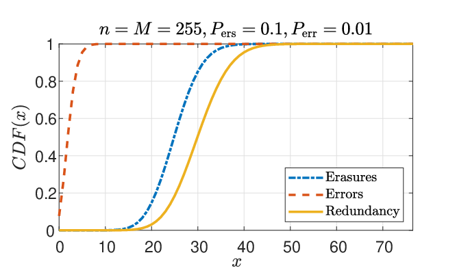
The trinomial CDF of , described in (16) is demonstrated in the left side of Fig. 6 (in yellow), compared to the binomial CDFs of erasures (blue dash-dot line) and errors (red dashed line), for and for .
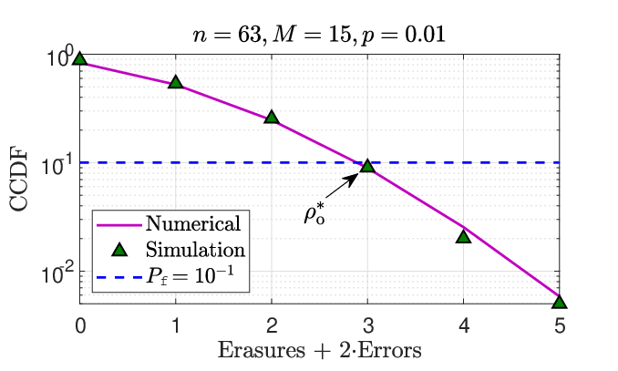
In the right side of Fig. 6, the trinomial complementary CDF (CCDF) is shown (in solid purple) for that are evaluated based on the analysis in Sections VI-A and VI-B for . This is compared with simulation results of encoding and decoding random words, using algebraic codes as described in Section III-C, while counting the number of erasures and twice the number of errors and evaluating the same CCDF (triangle markers). The required outer redundancy is also marked (horizontal dashed line) for , as the lowest value in x-axis for which the CCDF is lower than .
To see the interaction between the inner and outer codes, and to get the idea of their joint optimization, we plot in Fig. 7 some of the interesting variables defined earlier in the section. We first fix the alignment parameters , and validation parameter . Then we plot, as a function of the inner-code dimension , the probabilities (circle markers) and (square markers), for . Both of these probabilities are monotonically non-decreasing as the inner code gets weaker. We also plot the required outer redundancy (17) ( markers, right y-axis) to achieve . The code designer is to choose the combination of and that minimizes the compression rate, which is in this setup. The plot also reveals a floor value for the erasure probability, attributed to failed proper alignments, which cannot be improved by strengthening the inner code.

In Fig. 8, we compare the compression rate of the proposed scheme (for ) to the ubiquitous ORCOM algorithm [33]. For this comparison we use the standard measure of compression ratio in units of bits per base-pair (bpb). Without compression, each base-pair consumes bits, so the compression rate defined in Proposition 3 is simply the plotted bpb divided by . We use read size of base pairs for both schemes, which implies an inner-block size of bits in our scheme. For ORCOM, the compression ratios (taken from[34]) strongly depend on the sequencing coverage [35] (the average number of appearances of a specific symbol from the genome), due to its reliance on internal similarities. Our proposed scheme, in contrast, does not need high coverage, and is shown to achieve comparable rates, even when evaluated on synthetic DNA sequences that have higher entropy. Working at low coverages has significant advantages in complexity and latency.

Finally, in Fig. 9 we show simulation results of alignment and inner-decoding success probability of the proper alignment for the original (Algorithm 2) and modified (Algorithm 3) schemes, as a function of the deletion fraction out of the total number of errors. For both curves, we use the same inner code with parameters , , while only modifying the (sub)-candidate selection and the inner-decoding procedures, as described in Algorithm 3. It is clearly seen that the modified scheme can much better handle deletion errors with significant fractions.

VII Further Extensions
VII-A Multiple Deletions Compensating Distance
It is possible to extend the shift compensating distance to deal with multiple deletions in the same read.
Definition 32
. Let , and let
The shift compensating distance of order is defined by
It is noted that a greedy approach can be employed, that is for every
where . Under reasonable conditions (e.g. small substitution probability, non-consecutive deletions), it is expected that . Such a greedy approach can be highly advantageous over other metrics since it can be computed in linear time. An exact analysis of the conditions for the greedy approach to match the optimal one is outside the scope of this work.
VII-B Modifying To Single-Insertion
In this sub-section we briefly describe the slight modifications needed to adapt the single-deletion scheme to a single-insertion scheme. The basis for this adaptation is in the fact that an insertion made in the reference is equivalent to a deletion made in the read. For alignment with insertion in the reference, it would have been natural to reverse the roles of the read and reference in the shift compensating distance, i.e., using (where now ). Nevertheless, since only the read identifier of is sent to the decoder for alignment, this is not possible since the the decoder does not have consecutive indices of . Instead, we can define a cumulative Hamming distance with negative shifts, as follows
cf. Definition 8. We can now use to obtain a shift-compensating distance with a single insertion. For inner decoding we use the insertion ball of every candidate , as a sub-sequence of of length . From this point, the same decoding process as described in Section V-D is performed.
VIII Conclusions
In this paper we addressed the problem of compressing DNA-sequencing reads generated from a genome, while a closely similar reference is available at the decoder side. Specifically, we developed a distributed-source-coding scheme supporting an alignment process at the decoder. As a model for differences between the reference and the reads, we studied both substitutions-only and multiple substitutions with a single deletion (SDMS). For both models we provided decoding algorithms and probabilistic analysis of success probability. For the SDMS model we also introduced a novel alignment metric that is both efficient to evaluate and proven to have good rejection of false alignments. As some interesting topics for future research, we suggest the following problems:
- 1.
Adapting the scheme to optimally suit more complex statistical models of realistic genomic sequences.
- 2.
Developing an efficient algorithm for the calculation of the shift-compensating distance of order , along with its performance analysis.
- 3.
Modifying the scheme to support both deletions and insertions (in the same or different reads).
Acknowledgment
The authors would like to thank distinguished Prof. Jacob Ziv for valuable discussions and ideas.
References
- [1] A. S. Motahari, G. Bresler, and D. N. C. Tse, “Information theory of DNA shotgun sequencing,” IEEE Trans. on Information Theory, Vol. 59, No. 10, 2013.
- [2] Z. Zhu, Y. Zhang, Z. Ji, S. He, and X. Yang, “High-throughput DNA sequence data compression,” Briefings In Bioinformatics, Vol. 16, No. 1. 1-15, 2013.
- [3] N. S. Bakr and A. A. Sharawi, “DNA lossless compression algoirthms: Review,” American Journal of Bioinformatics Research, 3(3), 2013.
- [4] M. Hosseini, D. Pratas, and A. J. Pinho, “A survey on data compression methods for biological sequences,” Information 7, 56, 2016.
- [5] D. Slepian and J. K. Wolf, “Noiseless coding of correlated information sources,” IEEE Trans. on Information Theory, Vol. IT-19, No. 4, 1973.
- [6] A. Wyner, “Recent results in shannon theory,” IEEE Trans. on Information Theory, Vol. 20, No. 1, 1974.
- [7] S. S. Pradhan and K. Ramchandran, “Distributed source coding using syndromes (discus): Design and construction,” IEEE Trans. on Information Theory, Vol. 49, No. 3, 2003.
- [8] T. Uyematsu, “An algebraic construction of codes for slepian-wolf source networks,” IEEE Trans. on Information Theory, Vol. 47, No. 7, 2001.
- [9] A. Orlitsky and K. Viswanathan, “One-way communication and error-correcting codes,” IEEE Trans. on Information Theory, Vol. 49, No. 7, 2003.
- [10] Y. Minsky, A. Trachtenberg, and R. Zippel, “Set reconciliation with nearly optimal communication complexity,” IEEE Trans. on Information Theory, Vol. 49, No. 9, 2003.
- [11] A. Aaron and B. Girod, “Compression with side information using turbo codes,” Proceedings of IEEE Data Compression Conference, 2002.
- [12] M. Sartipi and F. Fekri, “Distributed source coding in wireless sensor networks using ldpc coding: The entire slepian-wolf rate region,” IEEE Wireless Communications and Networking Conference, 2005.
- [13] Y. Cassuto and J. Ziv, “Efficient compression of long arbitrary sequences with no reference at the encoder,” IEEE Trans. on Information Theory, Vol. 67, No. 1, 2021.
- [14] S. Wang, X. Jiang, F. Chen, L. Cui, and S. Cheng, “Streamlined genome sequence compression using distributed source coding,” Cancer Informatics. Supplementary Issue: Computational Advances in Cancer Informatics, 2014.
- [15] J. J. Shao, “Genome sequence compression algorithm based on the distributed source coding,” 6th International Conference on Machinery, Materials, Environment, Biotechnology and Computer (MMEBC), 2016.
- [16] M. Bossert, “Channel coding for telecommunications,” Wiley, 1999.
- [17] A. F. Wright, “Genetic variation: Polymorphisms and mutations,” Encyclopedia of Life Sciences, John Wiley and Sons, 2005.
- [18] C. Lottaz, C. Iseli, C. Jongeneel, and P. Bucher, “Modeling sequencing errors by combining hidden markov models,” Bioinformatics, Vol. 19, Suppl. 2, 2003.
- [19] S. Lin and D. Costello, “Error control coding, 2nd edition,” Pearson-Prentice Hall, 2004.
- [20] O. Amrani and Y. Be’ery, “Bounded-distance decoding: Algorithms, decision regions, and pseudo nearest neighbors,” IEEE Trans. on Information Theory, Vol. 44, No. 7, 1998.
- [21] E. R. Berlekamp, Algebraic Coding Theory, revised 1984 editon. Laguna Hills CA: Aegean Park Press, 1984.
- [22] J. H. Jeng and T. K. Truong, “On decoding of both errors and erasures of a reed-solomon code using an inverse-free berlekamp-massey algorithm,” IEEE Trans. on Information Theory, Vol. 47, No. 10, 1999.
- [23] V. I. Levenshtein, “Binary codes capable of correcting deletions, insertions, and reversals,” Soviet Physics Doklady, 1966.
- [24] H. Xin, J. Greth, J. Emmons, G. Pekhimenko, C. Kingsford, C. Alkan, and O. Mutlu, “Shifted hamming distance: A fast and accurate simd-friendly filter to accelerate alignment verification in read mapping,” Bioinformatics, 31(10), 2015.
- [25] E. Čech, M. Katětov, and P. t. Aleš, “Point sets,” Academia, Publishing House of the Czechoslovak Academy of Sciences, 1969.
- [26] P. Forrest, “The identity of indiscernibles,” The Stanford Encyclopedia of Philosophy, 2008.
- [27] C. Kusters and T. Ignatenko, “DNA sequence modeling based on context trees,” Proc. of the 36th WIC Symposium on Information Theory, 2015.
- [28] S. K. Leung-Yan-Cheong, E. R. Barnes, and D. U. Friedman, “On some properties of the undetected error probability of linear codes,” IEEE Trans. on Information Theory, Vol. IT-25, No. 1, 1979.
- [29] M. G. Kim and J. H. Lee, “Undetected error probabilities of binary primitive bch codes for both error correction and detection,” IEEE Trans. on Communications, Vol. 44, No. 5, 1996.
- [30] P. Rybin and V. Zybaloc, “On the upper bound on undetected error probability for ldpc code,” IEEE International Symposium on Information Theory (ISIT), 2014.
- [31] G. Boole, “The mathematical analysis of logic,” Philosophical Library, 1847.
- [32] Y. Gershon and Y. Cassuto, “Distributed source coding of fragmented genomic sequencing data,” IEEE International Symposium on Information Theory (ISIT), 2021.
- [33] S. Grabowski, S. Deorowicz, and L. Roguski, “Disk-based compression of data from genome sequencing,” Bioinformatics, 31(9), 2015.
- [34] A. A. Ginrat, J. Hui, K. Zhu, I. Numanagic, T. A. Courtade, S. Cenl Sahinalp, and D. N. Tse, “Optimal compressed representation of high throughput sequence data via light assembly,” Nature Communications, 2018.
- [35] I. Illumina. (2021) Sequencing coverage in next generation sequencing. [Online]. Available: https://www.illumina.com/science/technology/next-generation-sequencing/plan-experiments/coverage.html
- [36] R. M. Roth, “Introduction to coding theory,” Cambridge University Press, 2006.
- [37] E. A. Codling, M. J. Plank, and S. Benhamou, “Recent results in shannon theory,” Journal of Royal Society Interface, 2008.
- [38] K. Siegrist. (2020) Statistics libertexts, the simple random walk. [Online]. Available: https://stats.libretexts.org/Bookshelves/Probability_Theory/Probability_Mathematical_Statistics_and_Stochastic_Processes_(Siegrist)/11%3A_Bernoulli_Trials/11.06%3A_The_Simple_Random_Walk
- [39] O. Eğecioğlu and A. King, “Random walks and catalan factorization,” CiteSeer, 1999.
Appendix A Proof of Proposition 28
Proof:
A code with minimum distance can correct up to erasures and errors as long as [36]. For an MDS code, the minimum distance satisfies . Therefore, whenever a perfect reconstruction will occur, i.e. . As described in Proposition 4, we require a probability of at least for that event, i.e. . is the set of triplets for which their sum equals and , and enumerates the number of such possible combinations of reads, implying (16). Finally, the minimal value of satisfying the requirement is . ∎
Appendix B Simple Random Walks Properties
Let be an i.i.d sequence of random variables for which . Then, is called a simple random walk in one dimension. We further define . A specific sequence is called a path. It is a well known result (e.g.[37]) that the probability distribution of is given by . The reflection principle is a known property stating that for every path there is a bijection to another path for which the sub-path is reflected with respect to . The next lemma follows.
Lemma 33
. Let be the walk’s maximal value up to step . Then,
Proof:
See [38] for detailed proof. ∎
Lemma 34
. Let denote the walk’s maximal value and the first step index it was attained up to step , respectively. Then,
Proof:
We have
Now,
and
where the second term in the last equality is due to the reflection principle. Overall, we get the desired expression. ∎
Appendix C Proof of Theorem 12: Distribution of the Shift-Compensating Distance
Define the random variables and . We have
We denote as the number of length- sequence pairs subject to the conditions in its arguments. With no conditions, . We further denote by the number of sequence pairs corresponding to a particular random walk sequence with , and by this number when the particular random walk has both and . Additionally, we denote as the number of length- random walk sequences with and , where the former counts walks without and the latter with null steps. A third argument appearing in , or to the right of the in , represents the number of null steps in the random walk. We can now write
From here, we can split the sequences counting up to and after step , where: (i) the left random walk (up to ) has , (ii) the right random walk (after time , whose value is shifted to start at ) has , and (iii) the function is independent from , and satisfies . Hence,
We now write , since we can eliminate the zeros, evaluate a standard random walk, and multiply by the number of ways to place zeros along the sequence, excpet for the last step (which must be 1 since it attains the maximum).
Similarly, , where in this case there is no requirement on the last step. Hence,
Let be the processes for which . Let , and let be obtained from after removing the null steps. Finally, let be the corresponding (-),(+) walks (derived from in the non-null steps), such that . We now add a condition on the right random walk in its final step, which can take the values . We also denote .
| (18) | ||||
We can now enumerate the different terms in the sum above.
For each step for which , we separate between a type-I zero for which (no increments to in this step), and a type-II zero for which (both increase by 1). For the non-null steps up to we have and , hence and . Moreover, since determines the number of steps up to for which , there must be type-II zeros (since there are negative steps), and therefore type-I zeros up to step . Now, is obtained from counting the possible ways to place type-II zeros and type-I zeros from the zeros, i.e. . For the non-null steps after , we use the following lemma.
Lemma 35
. For a non-positive simple symmetric random walk, the number of possible sequences with negative steps and positive steps is
Proof:
The proof is based on similar considerations as in the proof of Theorem 1 in [39], with a reversal of roles between positive and negative steps. ∎
Based on this lemma, we get
Using similar considerations as above, we get that there are type-II zeros and type-I zeros after step , where . Again, by counting the number of possible placements of zeros we get that .
By substituting all of the above into (18), collecting binomial terms to multinomial terms and summing over from to , we complete the proof.