Impact of Point Spread Function Higher Moments Error on Weak Gravitational Lensing II: A Comprehensive StudyImpact of Point Spread Function Higher Moments Error on Weak Gravitational Lensing II: A Comprehensive Study–D
Abstract
Weak lensing is one of the most powerful probes for dark matter and dark energy science, although it faces increasing challenges in controlling systematic uncertainties as the statistical errors become smaller. The Point Spread Function (PSF) needs to be precisely modeled to avoid systematic error on the weak lensing measurements. The weak lensing biases induced by errors in the PSF model second moments, i.e., its size and shape, are well-studied. However, Zhang et al. 2021 showed that errors in the higher moments of the PSF may also be a significant source of systematics for upcoming weak lensing surveys. Therefore, this work comprehensively investigate the modeling quality of PSF moments from the to order, and propagate the PSFEx higher moments modeling error in the HSC survey dataset to the weak lensing shear-shear correlation functions and their cosmological analyses. The overall multiplicative shear bias associated with errors in PSF higher moments can cause a shift on the cosmological parameters for LSST Y10, while the associated additive biases can induce uncertainties in cosmology parameter inference for LSST Y10, if not accounted. We compare the PSFEx model with PSF in Full FOV (Piff), and find similar performance in modeling the PSF higher moments. We conclude that PSF higher moment errors of the future PSF models should be reduced from those in current methods, otherwise needed to be explicitly modeled in the weak lensing analysis.
Keywords:
methods: data analysis; gravitational lensing: weak1 Introduction
Weak gravitational lensing, or weak lensing, is the slight deflection of the light from distant objects by the gravitational effect of nearby objects. Weak lensing leads to a mild change in the object’s shape, size and flux, and it is a powerful probe of the dark matter distribution of the Universe due to its sensitivity to the gravitational potential along the line of sight (Hu 2002; Huterer 2010; Weinberg et al. 2013). To date, the most promising way of measuring weak lensing is to measure its coherent effects on the galaxy shape, i.e., the weak lensing shear. Weak lensing can be caused by a nearby massive galaxy or cluster, i.e., as measured using galaxy-galaxy lensing (Velander et al. 2014; Zu & Mandelbaum 2015; Prat et al. 2018, e.g.,); or by the large-scale structure of the Universe, as measured using cosmic shear (Hamana et al. 2020; Asgari et al. 2021; Amon et al. 2021, e.g.,).
The coherent galaxy shape distortions caused by weak lensing are currently measured using millions, in the future even billions, of galaxies in large astronomical surveys. The “Stage III” cosmological surveys (Albrecht et al. 2006) that started in the previous decade provided weak lensing observation that moved the field forward substantially; these include the Dark Energy Survey (Dark Energy Survey Collaboration et al. 2016, DES;), the Kilo-Degree Survey (de Jong et al. 2017, KiDS;), and the Hyper Suprime-Cam survey (Aihara et al. 2018a, HSC;). In the near future, “Stage IV” surveys will begin to observe at greater depth and/or area than the previous generation; the Stage IV surveys include the Vera C. Rubin Observatory Legacy Survey of Space and Time (Ivezić et al. 2019; LSST Science Collaboration et al. 2009, LSST;), the Nancy Grace Roman Space Telescope High Latitude Imaging Survey (Spergel et al. 2015; Akeson et al. 2019) and Euclid (Laureijs et al. 2011). These new surveys will provide greater statistical precision in the measurements, and therefore demand greater control of systematic uncertainties in weak lensing.
The Point Spread Function (PSF) is the function that describes the atmospheric turbulence, telescope optics, and some detector effects (Anderson & King 2000; Piotrowski et al. 2013) on a point source image. PSF modeling algorithms reconstruct the PSF at the position of the stars, and interpolate the model to arbitrary positions on the image, e.g., PSFEx (Bertin 2011), or to positions on the sky, e.g., Piff (PSF in Full FOV; Jarvis et al. 2021).
The raw light profile of the galaxies is convolved with the PSF, changing their observed shapes and sizes. Since measuring weak lensing signals relies heavily on measuring the coherent galaxy shape distortions, modeling the PSF correctly is fundamental for controlling weak lensing systematics. Failure of the PSF model to represent the true PSF causes systematic errors in the inferred galaxy shapes and weak lensing shears. Previous studies have developed a formalism that cleanly describes how the errors in modeling PSF second moments, i.e., the shape and size, affect the galaxy shape measurement and weak lensing shear inference (Hirata & Seljak 2003; Paulin-Henriksson et al. 2008; Rowe 2010; Jarvis et al. 2016, e.g.,). There is also a formalism that describes how the PSF second moment errors further propagate to the weak lensing observables (shear-shear correlations), using the “-statistics” (Rowe 2010; Jarvis et al. 2016).
However, the aforementioned formalism, which is commonly used for quantifying the quality of PSF modeling, does not consider the impact on weak lensing shear caused by errors in the higher moments, i.e., moments with order higher than the second, of the PSF model. In Schmitz et al. 2020, excess multiplicative and additive shear bias is found in addition to the predictions of the second moment formalism, for Euclid’s PSF. A previous study by Zhang et al. 2021 (hereafter ZM21) explored this topic by carrying out shape measurement experiments, with the radial kurtosis of the PSF intentionally mis-modeled, while preserving the PSF second moments. They found that errors in the PSF radial kurtosis can induce a multiplicative bias in the inferred weak lensing shear. They also found that for parametric galaxy models based on the COSMOS survey, and for PSF radial kurtosis errors as in the HSC public data release 1 (Aihara et al. 2018b, PDR1;) PSF models from PSFEx (Bertin 2011), the PSF radial kurtosis error can cause a redshift-dependent multiplicative shear bias at the level of the LSST Y10 requirement (The LSST Dark Energy Science Collaboration et al. 2018), thus motivating further research on this topic.
In this paper, we want to extend the understanding from ZM21 in several ways: (a) include a wider range of PSF higher moments, which might induce both multiplicative and additive shear biases; (b) propagate the biases into the common weak lensing data vector, the two-point correlation function (2PCF) , and to cosmological parameter estimates; (c) include Piff, which might provide some estimate of how algorithm-dependent the errors in PSF higher moments are, and might serve as a better example of an algorithm that will be used for LSST.
We introduce background material, including the weak lensing shear, PSF higher moments, and shapelet decomposition in Section 2. In Section 3, we describe the HSC datasets in this work for measuring the PSF higher moments, and show the results of the PSF modeling quality on the second and higher moments for two PSF models, PSFEx and Piff. In Section 4, we describe the methodology of single galaxy simulations, including simulation workflow, galaxy and PSF profiles, and how we change the PSF higher moments with the aid of shapelet decomposition. We also show the results based on these single galaxy simulations. In Section 5, we combine the results from Section 3 and 4 to further propagate the systematics induced by PSF higher moment errors to the weak lensing 2PCF, and its associated cosmology analyses by Fisher forecasting. In Section 6, we discuss the implications of our results for weak lensing with future imaging surveys.
2 Background
In this section, we describe the background of this paper. In Section 2.1, we introduce the formalism to quantify the weak lensing shear. In Section 2.2, we introduce the method for measuring the higher moments of PSFs. We then introduce the radial shapelet decomposition, used as a basis in which we expand any given PSF light profile, in Section 2.3.
2.1 Weak Lensing
Weak gravitational lensing, or weak lensing, is the coherent gravitational distortion on background (source) galaxy flux, size, and shape by foreground (lens) objects. The lens can be any massive object, e.g., a galaxy cluster, or the cosmic large-scale structure. Weak lensing is a powerful observable because of its sensitivity to the matter distribution along the line of sight (Hu 2002; Huterer 2010; Weinberg et al. 2013). In this paper, we are interested in the cosmic shear, which is the coherent distortion of the source galaxy shapes by the large-scale structure of the Universe, resulting in a nonzero two-point correlation function of galaxy shapes. The distortion of the galaxies by the weak lensing shear is determined by the reduced shear , which is a combination of the shear and the convergence (Mandelbaum 2018). describes the shear along the x- or y-axes, while describes the shear along an angle defined by growing counterclockwise from the x-axis on the image. Here the x-y axes are aligned with the local (RA, Dec) axes on the sky.
For a cosmological weak lensing analysis, it is useful to measure the weak lensing two-point correlation function (Miralda-Escude 1991), also referred to as the 2PCF. We can calculate the shear along a chosen angular vector connecting two galaxies, with polar angle , by , and to by . The shear 2PCF is computed by
| (1) |
Since the weak lensing shear is isotropic (statistically speaking), the is integrated over the polar angle and presented as a function of the angular distance .
The weak lensing shear 2PCF as measured through is sensitive to the coherent change in galaxy shapes due to large-scale structure (Schneider et al. 2002), though it is contaminated by intrinsic alignments (Croft & Metzler 2000; Heavens et al. 2000; Troxel & Ishak 2015; Joachimi et al. 2015, e.g.,), i.e., the correlated galaxy alignments due to local effects such as tidal fields.
Estimating shear accurately is a key step in any cosmological analysis of weak lensing data. Shear biases are commonly modeled as two terms, the multiplicative bias and the additive bias (Heymans et al. 2006; Massey et al. 2007a), which enter the estimated shear as
| (2) |
where denotes the estimated shear. Systematic biases in the estimated shear must not exceed a certain portion of the statistical error to avoid substantial biases in the reported constraints on the cosmological parameters compared to those that would ideally be recovered. We are particularly interested in a redshift-dependent multiplicative bias; as suggested in Massey et al. 2013, a redshift-dependent multiplicative bias can bias the inferred dark energy equation of state parameter from weak lensing. This is motivated since ZM21 found that the shear response to the PSF higher moment errors depends on the galaxy properties, which means that the galaxy ensemble in each tomographic bin will respond differently to the same PSF higher moment error. In The LSST Dark Energy Science Collaboration et al. 2018, the redshift-dependent multiplicative bias is parameterized by in
| (3) |
where is a non-zero average multiplicative bias over redshift. Error budget requirements are placed on the upper bound of the absolute value of multiplicative biases for weak lensing surveys (Jarvis et al. 2016; Mandelbaum et al. 2018). Taking LSST Y10 as an example (The LSST Dark Energy Science Collaboration et al. 2018), the requirement on the redshift-dependent multiplicative bias, which is the difference in across the full source redshift range, is 0.003. This motivates detailed studies on the connection between weak lensing shear systematics and other factors, including the PSF higher-moment modeling error (ZM21 and this work). Note that we only discuss the PSF-induced multiplicative shear biases in this work, without other sources of redshift-dependent multiplicative biases (MacCrann et al. 2022, e.g.,).
2.2 Moment Measurement
In this section, we introduce the methods for measuring higher moments of the PSF. Firstly, we define the adaptive second moment for a light profile,
| (4) |
where , , or . Here is the image intensity, where is the image coordinate with origin at the centroid of . in Eq. (4) is the adaptive Gaussian weight, which has the same second moments as the light profile (Hirata & Seljak 2003), defined by
| (5) |
The second moment size and shape and can then be calculated from the second moments using
| (6) | ||||
| (7) | ||||
| (8) |
Here is the determinant of the second moment matrix. From Eqs. (6)–(8), we can solve for the weighted second moments given the weighted shape and size , which are measured using the HSM module11 1 https://galsim-developers.github.io/GalSim/_build/html/hsm.html (Hirata & Seljak 2003; Mandelbaum et al. 2005) in GalSim (Rowe et al. 2015).
Based on the second moments, we also define a standardized coordinate system in Eq. (9); this is the coordinate system where the profile has zero second moment shape , defined in Eqs. (7)–(8), and second moment size , defined in Eq. (6). The standardized coordinate system can be determined via a linear transformation of the image coordinate system as follows:
| (9) |
The standardized adaptive higher moment, , is then defined by
| (10) |
For the th moments, takes any value between to , and . We choose to measure PSF higher moments in the standardized coordinate system instead of , as such quantities are scale and shape independent, assuming the PSF is well-sampled. The weight is applied to suppress image noise at large radii during the measurement process. The denominator is the normalizing factor, such that the higher moments will not depend on the amplitudes of the weight and the image.

Throughout this paper, we define the biases on the moment as
| (11) |
where is the moment of the model PSF, and is the moment of the true PSF. Note that we refer to the standardized higher moments as the “higher moments” throughout this paper.
2.3 Shapelet Decomposition
The shapelet decomposition is an expansion of a two-dimensional image with the eigenfunctions of the 2D quantum harmonic oscillator as the basis functions. This basis function is also referred to as the Laguerre Function with Gaussian weight. This method was used to expand the galaxy and PSF profile in Massey & Refregier 2005 and used to measure weak lensing shear in Massey et al. 2007b. For detailed explanations of shapelet expansions, see also Bernstein & Jarvis 2002. In this study, we use the shapelet decomposition implemented in GalSim22 2 https://github.com/GalSim-developers/GalSim (Rowe et al. 2015).
The shapelets basis functions are parameterized by a single parameter: the length scale . After determining the value of for the image, the image can be decomposed into a series of shapelet coefficients , indexed by and . We also defined two more indices, i.e., the order and the spin number . The PSF image can be expanded by the basis functions of the shapelet coefficients ,
| (12) |
where is the Laguerre Function with Gaussian weight, i.e., the radial shapelet basis in a polar coordinate system with radius and polar angle ,
| (13) |
The is the Laguerre Polynomial. Fig. 1 shows the first 15 basis images of that we used to decompose the PSF. For a given order , there are shapelet basis functions. Due to conjugate pairings, of the shapelet coefficients are identical to . Therefore, to expand a real image, we have distinct shapelet basis functions for order that satisfy .
To determine the length scale , we carried out the following experiment: We decomposed the PSF with different length scales ; kept the 40 leading s of the shapelet series; reconstructed the image using the first forty ; and measured the residual of this reconstruction. We found that to minimize the absolute value of the residual of the reconstruction, the length scale should be set to the weighted second moment of the PSF defined in Eq. (6). This rule was found to be true on both the Gaussian and Kolmogorov profiles. We therefore adopted this approach throughout this work.
3 Data
In this section, we introduce the data from the Hyper Suprime-Cam survey (Aihara et al. 2018a, HSC;) to study how well current PSF models recover PSF higher moments. We inspected two datasets, one for PSFEx and one for Piff. For both datasets, we used the coadded images of bright stars as the true effective PSF, and compared them with the PSF model at the bright stars’ positions. The PSFEx and Piff star catalogs are described in Sections 3.1 and 3.2, respectively. We describe the measurement results of the PSF higher moments error in Section 3.3.
3.1 PSFEx Dataset
The dataset for quantifying the modeling quality of PSFEx is the star catalog of the first HSC public data release (Aihara et al. 2018b, PDR1;). The PSFEx model in this study was generated by the HSC pipeline (Bosch et al. 2018) with a modified version of PSFEx (Bertin 2011); see Section 3.3 of Bosch et al. 2018 for more details. We used all six fields in the PDR1 survey to inspect the PSF higher moments, instead of just the GAMA_15H field as in ZM21. Our star selection process for the PSFEx is detailed in Section 3.4.1 in ZM21, so we only summarize it briefly here.
We adopted the “basic flag cuts” from Table 3 of Mandelbaum et al. 2018, with iclassification_extendedness set to 0 to identify non-extended objects. These flag cuts eliminate objects that are contaminated or affected by exposure edges, bad pixels, saturation or cosmic rays, and reduce the number of selected stars to . We adopted a signal-to-noise ratio (SNR) cut to reduce noise in the PSF higher moments measurement, which further reduced the sample size to . The SNR cut was determined so that the statistical uncertainty in the PSF radial fourth moments of the star images is (ZM21), avoiding a scenario where the higher moments are dominated by the image noise. The i-band magnitudes of the selected stars are between 18 to 20, a regime in which the correction for the brighter-fatter effect (Bosch et al. 2018) is highly effective as shown in Section 4.2 of Mandelbaum et al. 2018. The SNR selections are only done for our PSF modeling inspection, not when running the PSF modeling step.
ZM21 identified the need for a cut iblendedness_abs_flux to address the fact that the moment measurements of blended objects are biased. In this work, that cut reduced the sample size to . Finally, we also excluded stars with a close neighbor within arcmin of their centroids using a k-d tree. At the end of the selection process, we had stars, around four times the amount in ZM21 since we used all six HSC fields. The number density of the PSFEx star dataset is arcmin-2. Examples of moment residual maps for PSFEx are shown in Appendix A.
3.2 Piff Dataset
We measured the performance of Piff (Jarvis et al. 2021) on the HSC data in order to compare with PSFEx. Piff was used as the PSF modeling algorithm for the DES Y3 dataset and performed better than previous DES PSF models, especially at modeling continuous trends across multiple detectors. Piff has been run on the HSC Release Candidate 2 (RC2)33 3 Detailed description of the RC2 dataset can be found in https://dmtn-091.lsst.io/v/DM-15448/., which consists of two HSC SSP-Wide tracts and one HSC SSP-UltraDeep tract. We used version 1.1.0 of Piff. It modeled PSFs in the image coordinate system, instead of in the WCS coordinates, with pixel scale equal to the native pixel scale ( arcsec). The model kernel size is pixels. The PSF was interpolated with a second order polynomial. We used outlier rejection with nsigma and max_remove . We refer the readers to Jarvis et al. 2021 for a detailed explanation of these settings. The RC2 dataset is reprocessed biweekly using the latest version of Rubin’s LSST science pipelines (Jurić et al. 2017). We inspected the PSF modeling quality on the two wide-field tracts, which correspond to an area of deg2 (each tract of the HSC data is roughly 2).
The star selection differs from that used for the PSFEx dataset: we used the pre-selected Piff candidate stars with SNR, without the need for the blending flux and close-neighbor cut. By this criterion, we had in total 11366 stars and PSF models to compare. The number density of the Piff dataset is arcmin-1, about 13 per cent lower than that for PSFEx. Examples of moment residual maps for Piff are shown in Appendix A.
3.3 Measuring PSF Higher Moment Error


We used the postage stamp images of the selected stars as measures of the true PSF. We obtained the PSF models evaluated at the position of the stars, as the model PSF. We used coadded star images, for which the PSF models are a weighted coaddition of the PSF model in each exposure (Bosch et al. 2018). We measured the 22 higher moments, defined in Eq. (10), from the to the order with the method described in Section 2.2. We also measured the weighted second moments with the HSM (Mandelbaum et al. 2005) module of GalSim.
We measured the moment biases by subtracting the star PSF moments from the model PSF moments , as in Eq. (11). In Fig. 2, combining the measurements of the PSF higher moments for all of the selected stars in these datasets, we show the distributions of the PSFEx and Piff moment errors with box plots side by side. The whiskers of the plot show the ranges of the distributions, the boxes show the interquartile ranges, and the bars show the median. We can see from the box plots that the two PSF models have similar PSF second moment residuals, and the PSF sizes are positively biased in both models, as observed for PSFEx in Mandelbaum et al. 2018. We listed the mean of the moment residual for PSFEx and PIFF in Table 2.
We calculated the “bias fluctuation” field by
| (14) |
We then used the two-point correlation function (2PCF) to measure the cross-correlation of the bias fluctuations and ,
| (15) |
When and , Eq. (15) becomes the auto-correlation function of . We measured the 2PCFs of the PSF higher moment errors using TreeCorr44 4 https://github.com/rmjarvis/TreeCorr (Jarvis et al. 2004).
Because of the relatively small area of the Piff dataset, we only measured its one-point statistics (mean, covariance matrix, etc.), not its two-point statistics. Therefore, we can only compare Piff with PSFEx at the early analysis stage, rather than propagating to the weak lensing data vector contamination and biases in cosmological parameter estimates.
The version of Piff used for this work produces similar order-of-magnitude PSF moment residuals as PSFEx from the 2nd to the 6th moments. However, its median residuals on , , and are several times larger than those for PSFEx, which is important because those are the primary moments contributing to the shear bias. This finding is not surprising because the implementation of Piff integrated with Rubin’s LSST Science Pipelines has not been thoroughly tuned, and in particular, none of its testing has focused on its optimization for accurate recovery of PSF higher moments. The results for Piff in Fig. 2 motivate further algorithm development and tuning, by providing additional metrics toward which to optimize in addition to the 2nd moments. In Appendix A.2, we show an apples-to-apples comparison between Piff and PSFEx on the RC2 dataset; the results further motivate the optimization of Piff toward minimizing PSF higher moment residuals.
In Fig. 3, we show the correlation matrix between the true PSF moments and their residuals for PSFEx (upper) and Piff (lower panel). We see a chequered-flag pattern in the correlation matrices. The true moments with the same parity for both and are usually positively correlated, and likewise for the residuals. This results in a chequered pattern within the same order – the () and the () moments are correlated – as well as a bigger chequered pattern across the orders – between and orders, though the latter cannot be seen in our plots, since we are only showing and moments. There is an even larger scale pattern: the true moments and residuals for a given are typically anti-correlated with each other due to the impact of noise on the true moments. We also observe a significant anti-correlation between “t” and “r04”/ “r40” for PSFEx. This indicates that and are preferentially overestimated in areas of the survey with good seeing. This result is consistent with the findings of ZM21, but it is not seen in the Piff results because it does not perform oversampling for good-seeing images. However, the correlation matrix of Piff shows stronger anti-correlations between the true and the residual moments, which suggests that the model is relatively unresponsive to the true values.
There are some caveats regarding the results presented in this section: (a) Due to the way that HSC PDR1 reserves PSF stars randomly for each exposure, 97% of the stars in the PDR1 dataset were used to generate PSF models in more than one exposure before the coadding process Bosch et al. 2018, so we are potentially underestimating the systematic uncertainties from the PSF interpolation process. (b) The results in this paper may overestimate and compared to the real HSC cosmic shear catalog, as the anti-correlation between and and seeing suggested that PSFEx severely overestimated and in good-seeing parts of the survey, which were eliminated from the shear catalog (Mandelbaum et al. 2018). Later HSC releases Aihara et al. 2022 showed that the updated HSC coaddition method using the fifth-order Lanczos kernel did considerably better at modeling the PSF in good-seeing regions than the third-order Lanczos kernel in the first data release. Therefore, the modeling errors in the good-seeing fields are reduced for the later HSC three-year shear catalog Li et al. 2022. Given this resolution, we will not further investigate this particular issue.
4 Image simulation
In this section, we introduce the image simulations used in this study. The main purpose of the image simulation is to understand the shear response to the PSF higher moments modeling error, of which the methods and results are presented in this section.
We will briefly cover the parts that are similar to the image simulation process in Section 3.3 of ZM21 and focus on the details that are different from the previous paper. The general simulation workflow is introduced in Section 4.1, the galaxy profiles in Section 4.2. In Section 4.3, we introduce our method of manipulating PSF higher moments by changing the coefficients of the shapelet decomposition, and the PSF profiles used in this work in Section 4.4. We show the results of the shear response to the PSF higher moment errors with image simulations in Section 4.5.
4.1 Simulation Workflows
Fig. 4 introduces the general image simulation workflow. The top part of the figure shows the steps of the image simulation process for one parametric galaxy and PSF. We started with a galaxy profile and its 90- rotated pair (Massey et al. 2007a), an approach we used to reduce simulation volume by nullifying shape noise, for which the parameters will be introduced in Section 4.2. The two galaxy profiles were convolved with the true effective PSF, introduced in detail in Section 4.4; it includes the convolution with a pixel response function ( arcsec). The convolved profiles were then sampled at the centers of pixels, generating the postage stamp images. The image set for the rotated galaxy pair was fed into the shear measurement algorithm, which is the re-Gaussianization (Hirata & Seljak 2003) method implemented in the HSM module (Mandelbaum et al. 2005) in GalSim (Rowe et al. 2015). We do not use Metacalibration (Sheldon & Huff 2017; Huff & Mandelbaum 2017) as ZM21 showed that systematic biases in shear due to PSF modeling errors do not strongly depend on shear estimation methods. We used the average of the measured shears for the galaxy and its 90- rotated pair as the shear estimate for a given PSF. Finally, the difference between the two shear estimates , measured by the true PSF and the model PSF, provides the shear bias associated with the PSF higher moment bias .
The additive shear response to the higher moment error was estimated at by
| (16) |
To estimate the multiplicative shear bias generated by the PSF higher moment errors, we introduced another shear . Its estimated values for the true and model PSF, and their difference , were used to estimate the multiplicative biases as
| (17) |
There are some general settings that apply to all of our image simulations: we used GalSim (Rowe et al. 2015) to render the simulated images, all of which are noise-free postage stamp images with a pixel scale of arcsec, similar to the pixel scale of the Rubin Observatory LSST Camera (LSSTCam).
4.2 Galaxy Profile
| Index | Galaxy Type | Galaxy Parameters | PSF Parameters | ||
|---|---|---|---|---|---|
| 1 | Gaussian | arcsec | arcsec | ||
| 2 | Gaussian | arcsec | arcsec | ||
| 3 | Gaussian | arcsec | (0.0, 0.0) | arcsec | 0.005 |
| 4 | Sérsic, n=3 | arcsec | (0.0, 0.0) | arcsec | 0.005 |
| 5 | Gaussian | arcsec | arcsec | 0.005 | |
| 6 | Sérsic, n=3 | arcsec | arcsec | 0.005 | |
| 7 | Bulge+Disc | in Table 3 | FWHM arcsec | 0.005 |
Two types of galaxy profiles were used in this study. The simpler galaxies were simulated as elliptical Gaussian light profiles. Gaussian galaxies were used in preliminary tests to develop basic intuition about the shear biases induced by errors in the PSF higher moments. The more complex galaxy model was a bulge+disc galaxy, consisting of a bulge and a disc component. The bulge+disc model was used for more sophisticated tests that attempt to represent a more realistic galaxy population as in the cosmoDC2 catalog (Korytov et al. 2019a).
The Gaussian profiles were parameterized by their size and ellipticity . We used them for initial tests to understand the relationship between shear bias and PSF higher moment bias (linear or non-linear?), the type of induced shear bias (multiplicative or additive?), and to determine which PSF higher moments actually contribute to weak lensing shear biases. The galaxy and PSF parameters for these preliminary single galaxy simulations are shown in Table 1, with results shown in Section 4.5. All base PSFs used in these initial simulations were Gaussian profiles, except for the last row, which is a Kolmogorov PSF.
A more sophisticated galaxy profile we used is the bulge+disc galaxy, a classic model used by many studies (Allen et al. 2006; Simard et al. 2011, e.g.,). The bulges and disks in this work have common centroids. The bulge component was a de Vaucouleurs profile (de Vaucouleurs 1948), a Sérsic profile (Sérsic 1963) with , which means the surface brightness is proportional to , where is the distance from the centroid in units of its scale radius. The disk component was an exponential profile, i.e., the surface brightness is proportional to , or the Sérsic profile. Both components have independent size and shape parameters. The luminosity profile of the components of the bulge+disc galaxy was governed by two parameters: total luminosity and the bulge fraction (). The bulge+disc simulations allowed us to estimate the shear response to error in the PSF higher moments as a function of galaxy properties, which is an important input to the catalog-level simulations later in Section 5.3.

4.3 Moment-Shapelet Relation
Before introducing the PSF profile, we need a way to generate light profiles that differ in higher moments, introduced in Section 2.2, from the base PSF in ways that we can specify. Unfortunately, we do not know an analytical expression for a basis that has a one-to-one mapping with the higher moments. However, since the shapelet basis and the unknown moment response can be used to describe the same linear space, we can reconstruct the unknown basis through linear combinations of the known shapelet basis, described in Section 2.3.
To do so, we defined the Jacobian matrix
| (18) |
which is the generalized gradient of the moments with respect to the shapelet coefficients defined in Eq. (12). We ranked the shapelet coefficients and PSF higher moments according to the orders in Fig. 1 and Fig. 5 We then directly estimated the change in moment given the change in all shapelet coefficients ,
| (19) |
Since converges to zero at large for Gaussian-like profiles including ground-based PSFs, we were able to truncate the shapelet expansion at some finite order, making and finite-sized vectors and matrices.
To numerically measure of the PSF with higher moment , we first decomposed the PSF into a set of shapelet coefficients . Then we perturbed , and measured the higher moment after the perturbation. The Jacobian element was then estimated by
| (20) |
In Appendix B, we show a visualization of the Jacobian matrix that describes how PSF moments can be modified through changes in the shapelets coefficients.
In the next section, we introduce the PSF profiles in this paper, and describe how we use the Jacobian defined in this section to precisely change the PSF higher moments.
4.4 PSF Profile
In the image simulations, we created the true and model PSF based on a “base PSF”. We considered two base PSFs: Gaussian and Kolmogorov. Note that the base PSFs do not include the pixel response function, but the model and true PSFs do include it. The process to create the true and model PSF is shown in the orange box in Fig. 4.
To change the PSF moments using the technique described above, we first rendered an image of the base PSF including convolution with the pixel response function, and expanded that image by the shapelet decomposition implemented in GalSim (Rowe et al. 2015). We carried out the shapelet decomposition up to order , which corresponds to determining shapelet basis coefficients. To test that the shapelets decomposition is effectively representing the higher moments of the PSF profile, we confirmed that the fractional kurtosis error measured using the adaptive moments of the shapelets-reconstructed PSF compared to the original image is for Kolmogorov and for Gaussian, which is an acceptable precision for this study. The kurtosis is a good quantity for comparing higher moments, since (a) it is a combination of three moments (, , and ); (b) many other higher moments are zeros, and are not suitable for comparing fractional differences.
After representing the true PSF as an order shapelet series, we calculated the Jacobian that links the shapelet coefficients with the PSF higher moments. The Jacobian is defined by Eq. (18) and estimated by Eq. (20). In this study, we investigated the higher moments from to order, corresponding to moments. Together with the three second moments, the Jacobian is a matrix. As an example, the Jacobian for the first 15 moments and first 15 shapelet modes is shown in Fig. 16.
Before describing how to use to construct images with precisely modified higher moments, we first define our notation. The true and model PSF are represented as vectors of shapelet expansion coefficients and . The corresponding moment vectors are and .
Ideally, we only change one higher moment of the PSF at a time, by solving for in Eq. (19). However, because of the non-linearity of the moment-shapelet relationship, the higher moments will not change exactly according to when we add and . Therefore, we introduced multiple iterations until the target moment biases are achieved, specified in Algorithm 1. We defined as the difference between our target moment vector and the current moment vector, which is the quantity we want to minimize. We used the L2 norm to quantify the magnitude of , i.e., .
We used this algorithm to ensure that the moments of the new PSF model approach the target moments , so the new PSF model has moment biases that differ from those of the true PSF by . We set the default threshold for the error in moment change to be , and the algorithm usually took less than 5 iterations to converge for Gaussian and Kolmogorov PSFs. Note that we included the second moments in the moment bias vector and set them to zero. In this way, we actively verified that the model and true effective PSF have the same second moments.
Introducing one component of at a time enabled us to inspect the moment response from second to sixth order by taking the difference between the images before and after one moment is slightly biased, in Fig. 5. This also enabled us to quantify the impact on weak lensing shear associated with errors in the PSF model for a specific moment.
4.5 Shear Response to PSF Higher Moments
In this section, we show the results of the image simulation and shear measurement experiments described in Sections 4.1 to 4.4, using Gaussian PSFs and 90- rotated galaxy pairs. Using the single galaxy simulations, we can learn the following: (a) the form of the shear response to PSF higher moment errors – are they linear, quadratic, or even more complicated; and (b) the pattern of shear biases associated with PSF higher moment errors, including magnitude of the biases and symmetry in the response to particular moments. Item (b) is particularly useful as it permits dimensionality reduction to focus on only the key PSF moments in later experiments.
ZM21 found only multiplicative biases associated with the radial kurtosis error of the PSF model. In this study, we cannot assume that all biases will be multiplicative, since we introduced other moment errors. In Fig. 6, we show the additive shear biases due to in the and moments of the PSF model, with shown on top of each sub-plot. The galaxy and PSF parameters are given in row 1 of Table 1. Fig. 6 shows that the moments induce shear biases that are linear in the moment residuals, while moments induce shear biases that are non-linear in the moment residuals across the range of higher moment residuals seen in real data. We found that these curves can fit with a quadratic form. The shear response to the even moments is 2-3 orders of magnitude higher than to the odd moments, at a fixed . We also note that the shear responses to conjugate higher moments, such as and , have opposite signs. This is expected since the two moments are related through a 90- rotation, causing an opposite effect on the shear. The symmetries in the shear responses to PSF higher moment errors are further discussed in Appendix C. To reduce the size of the figure, we omitted the 5th and 6th moments, but they exhibit the same trends as the 3rd and 4th moments in terms of parity symmetry and different order of magnitude between shear biases for odd and even moments.
| Moment | |||
|---|---|---|---|
| (0,3) | () | () | -0.21(0.24) |
| (1,2) | () | () | 0.13(-0.04) |
| (2,1) | () | () | -0.07(-0.02) |
| (3,0) | () | () | 0.34(-0.09) |
| (0,4) | () | () | 1.35(2.52) |
| (1,3) | () | () | -0.01(-0.06) |
| (2,2) | () | () | -0.19(-0.16) |
| (3,1) | () | () | -0.0(-0.04) |
| (4,0) | () | () | 1.02(3.67) |
| (0,5) | () | () | -0.96(0.86) |
| (1,4) | () | () | 0.34(-0.13) |
| (2,3) | () | () | -0.2(0.09) |
| (3,2) | () | () | 0.33(-0.11) |
| (4,1) | () | () | -0.2(-0.13) |
| (5,0) | () | () | 1.5(-0.08) |
| (6,0) | () | () | 3.42(11.77) |
| (5,1) | () | () | -0.05(-0.18) |
| (4,2) | () | () | -0.16(0.49) |
| (3,3) | () | () | -0.02(-0.13) |
| (2,4) | () | (-) | -0.3(0.96) |
| (1,5) | () | () | -0.02(-0.18) |
| (0,6) | () | () | 1.6(16.72) |
Next, to measure both additive and multiplicative shear biases, we used the same galaxy and PSF sizes as in Fig. 6, but we varied the lensing shear applied to the galaxies (specified in row 2 of Table 1). In Table 2, we show the multiplicative and additive shear biases per unit of PSF higher moments biases and for the 3rd to 6th moments, at the average PSF higher moment biases. Similar to Fig. 6, the shear responses to the odd moments are at least two orders of magnitude smaller than the responses to the even moments. All even moments generate multiplicative shear biases, and they also strongly determine the additive biases. Notice that since the shear responds nonlinearly to the odd moments, the values for those moments in Table 2 depend on the PSF moment residuals. Based on the results from Section 3.3, we can simply estimate the order of magnitude of and for a typical galaxy as being on the order of to . A more precise estimate of the systematic biases for ensembles of galaxies will be provided in Section 5.3.
ZM21 showed that the galaxy-to-PSF size ratio is the most important factor that determines the shear response to the errors in modeling the PSF radial kurtosis. Here we checked the sensitivity of the additive and multiplicative shear biases induced by individual PSF higher moment errors to that size ratio. We explored this relationship by simulating Gaussian and Sérsic galaxies with various sizes, specified in rows 3 to 6 in Table 1. In Fig. 7, we show the additive (multiplicative) shear biases in the upper (lower) panel, as a function of the galaxy-to-PSF size ratio measured by the half light radii . We can see that the size ratio plays an important role, but the Sérsic index also affects the shear responses significantly, especially for large size ratios. This is consistent with the findings in ZM21. In Fig. 7, we note that the shear responses of Gaussian galaxies to the PSF third moments are non-monotonic, crossing the 0 reference line multiple times. The simulations in Fig. 6 corresponded to a galaxy-PSF size ratio of , for which the third moment responses of and happen to have the same sign. As seen in Fig. 7, the signs of the shear biases for the third moment residuals in Fig. 6 are not representative of many galaxy-to-PSF size ratios, and should not be over-interpreted. However, the small magnitude of the additive shear biases caused by third moment modeling errors in Fig. 6 are more generally applicable.
In the next section, we will combine the findings in this section and in Section 3 to estimate the systematic error in weak lensing observable and cosmology analyses associated with PSF higher moment errors.
5 Weak Lensing and Cosmology Analyses
In this section, we discuss the propagation of errors in shear to the weak lensing 2PCF, and further into cosmology. We first provide a general derivation of our approach in Section 5.1, and then describe an important practical issue – reducing the number of moments – in Section 5.2. We introduce the mock galaxy catalog we use for estimating systematics, the cosmoDC2 catalog (Korytov et al. 2019b), in Section 5.3. We further propagate the weak lensing shear systematics to cosmological parameter analysis using Fisher forecasts as described in Section 5.4.
5.1 General Error Propagation
Our discussion of how errors in the PSF higher moments affect the weak lensing 2PCF is based on two assumptions: (a) Each PSF higher moment may produce additive shear biases and multiplicative biases on the observed shear, . (b) The total multiplicative and additive bias and produced by simultaneous errors in multiple higher moments of the PSF can be expressed as the sum of the individual multiplicative and additive biases ,
| (21) | ||||
| (22) |
with uncertainties that are negligible for this work. The assumption (a) was illustrated in Section 4.5, and (b) was confirmed with an image simulation test, where 100 galaxies sampled from cosmoDC2 were assigned random PSF higher-moments residuals. That test showed that the absolute value of the differences between the two sides of Eqs. (21) and (22) for individual galaxies are . We have explicitly confirmed that for ensemble shear estimation, the error due to assumptions of linearity is further reduced to %. For the multiplicative biases, since , we can ignore the high-order correlations, and just focus on the first order expansion of the observed 2PCF of weak lensing shear. Additive biases can be written as the sum of their averages and fluctuations, . Combining the additive and multiplicative terms, we get the full expression for the observed weak lensing 2PCF between bins and ,
| (23) | ||||
where is the multiplicative bias defined in Eq. (3). Throughout this work, we ignored the spatial variation of the multiplicative bias, which as shown by Kitching et al. 2020 can enter the shear power spectrum at a lower level than the mean multiplicative bias.
As shown in Eq. (23), the additive shear bias terms have two effects. First, the observed 2PCF is shifted by a constant . Second, it is also shifted by the scale-dependent auto-correlation function of the zero-mean additive bias field . We explore the impact of these changes in subsequent sections.
5.2 Dimensionality Reduction for PSF Higher Moments
There are 22 correlated PSF moments from to order, and the high dimensionality of this dataset can pose challenges in understanding the main issues determining the weak lensing systematic biases. Therefore, dimensionality reduction to only the PSF higher moments that induce substantial shear biases is an important first step. Since this task is based on a rough estimate of the importance of individual PSF higher moments, we used simple models for this: both the galaxy and PSF in the dimensionality reduction process are Gaussian profiles.
Eq. (23) shows that multiplicative bias affects the weak lensing 2PCF through its total , which is a summation over all . We used the methods described in Section 4.1 to calculate as a function of the galaxy’s second moment . To roughly estimate , we used the of 44386 COSMOS galaxies with magnitude , and galaxy resolution factor (later defined in Eq. 27) as the input galaxy sizes. The second moments were computed after convolving with the Hubble PSF, but before convolving with our Gaussian PSF. The Gaussian PSF size was fixed at a Full Width at Half Maximum (or FWHM) of . Assuming the shear bias is proportional to the PSF moment bias, the multiplicative bias should be proportional to the moment bias as well. Therefore, we estimated the multiplicative bias associated with as
| (24) |
where the COSMOS galaxies are indexed by , and is the average moment bias of in the HSC data, as described in Section 3.3. The method to estimate was described in Section 4.1. We ranked the magnitude of the values of to estimate the importance of individual PSF moments. The importance is expected to be different for and , given different spatial patterns are involved in different moments.
The resulting multiplicative biases from this simplified simulation are shown in Fig. 8. Both the and results indicate that PSF higher moments with both and even (seven in total) determine the multiplicative shear bias. The total multiplicative biases are and , dominated by the contributions of 7 PSF higher moments.
The additive biases are more complicated as shown in Eq. (23), since we must calculate the weak lensing 2PCF to understand the importance of the moments. We designed the preliminary tests for the additive biases as follows: We used the PSF higher moments and their errors as a function of position in the HSC PDR1 from Section 3, and for the positions of bright stars in the PDR1 fields, we simulated a synthetic Gaussian galaxy with the average size and shape of the population from COSMOS catalog. We then measured the shear biases of the Gaussian galaxies with the PSF higher moments biases at these positions. We obtained the biases on the shear 2PCF directly from the shear bias at position , estimated by
| (25) |
As shown in Fig. 9, the additive bias on has a magnitude on tens of arcmin scales, which corresponds to a per cent additive systematics contribution at small scales, and a few per cent at large scales, which is significant enough to potentially affect cosmological inference. The sharp decrease at arcmin suggests that physical effects associated with the HSC field of view (FOV) are the cause of structural PSF systematic biases. However, is effectively zero.
Since each term in the additive biases on the 2PCF is associated with two different PSF moments (Eq. 23), the ranking of importance for the PSF moments is more complex in this case. We designed two different ranking system: (a) the front-to-back approach and (b) the back-to-front approach. In the front-to-back approach, we calculated the contribution of each term to the total additive bias , by integrating over from to arcmin. We ranked the contribution of a given moment by the total reduction in additive bias if we removed all terms that involve . After removing the highest-contributing PSF moment, we performed the same calculation and removed the next highest-contributing moment, until only one moment remains.
Similarly, for the back-to-front approach, we removed the least-contributing PSF moment first, after performing the same contribution calculation described above. We then removed the next least-contributing moment, until we were left with only one moment. These two approaches provided two rankings of the PSF moments that contribute from most to least to the weak lensing additive shear bias. We expect to obtain a reasonably consistent set of PSF moments from these two approaches. If the two results were to disagree, the conservative approach would be to use the inclusive set of moments considered important by either method.
We ranked the moments separately for and . In Fig. 10, we show the results of executing the dimensionality reduction process for additive shear bias outlined in Section 5.2. In the upper and middle panel, we show the ranking of the PSF moments’ contribution to and . We show both the “front-to-back method” and “back-to-front method”, described in Section 5.2. The relative rankings given by the two methods are slightly different, but the methods agreed about which moments we should discard. The moments that contribute the most strongly are four of the five moments: (4,0), (3,1), (1,3), (0,4), and all seven moments. We further separated those 11 moments into two groups depending on which shear component they affect ( or ). The moments in the () group are those with even (odd) values for both and . In the bottom panel, we show the additive biases on and contributed by all PSF higher moments, compared to just the contributions of the ‘ group’ and the ‘ group’. The plot shows that the ‘ group’ and ‘ group’ moments dominate the total additive shear biases, and therefore we can focus on just these higher moments.
After the dimensionality reduction of PSF higher moments, we only propagate the errors on the reduced moment set to the lensing signal in the analysis in subsequent sections. In other words, from this point on we only consider errors in 7 (11) PSF higher moments for the multiplicative (additive) biases.
5.3 Mock Catalog Simulations
To connect PSF higher moment errors with weak lensing systematics, we need a realistic galaxy catalog with galaxy properties and positional information. For this purpose, we used the cosmoDC2 catalog (Korytov et al. 2019a), as it is designed to match the galaxy population LSST is going to observe, with multiple validation tests against real datasets (Kovacs et al. 2021), and has sufficient area (440 2) for our purposes. We accessed the cosmoDC2 catalog using GCRCatalogs55 5 https://github.com/LSSTDESC/gcr-catalogs (Mao et al. 2018).
We estimated the multiplicative and additive shear biases for each individual galaxy in cosmoDC2 using two pieces of information: shear response to PSF higher moment errors, and a synthetic catalog of PSF higher moment errors, both described below.
5.3.1 Shear Response
The shear response to errors in PSF higher moments, , depends on the galaxy and PSF properties. We used a bulge+disc decomposition model for the galaxy, and determined the shear response as described in Section 4. To reduce the computational expense, we carried out simulations for a grid of bulge+disc model parameters that cover the majority of the cosmoDC2 galaxies, discarding per cent (large galaxies that do not contribute significant shear bias) outside of the grid. The free parameters in the grid are the half-light radius of the bulge , the half-light radius of the disc , and the bulge fraction , and the grid is linear in all three dimensions. We used the same bulge and disc shapes for all galaxies66 6 Our tests showed that using the same ellipticity for all galaxies generates 1 per cent error on the prediction of the ensemble shear biases, while saving tremendous computational time.. We set the size and shape of the Kolmogorov PSF to be constant. The pixel size is arcsec, like that of the Rubin Observatory LSST Camera. The range of bulge+disc parameters in the image simulation is in Table 3.
| Parameter | Range |
|---|---|
| Bulge | |
| Disc | |
| Bulge-to-total ratio | |
| Bulge shape | |
| Disc shape | |
| PSF FWHM |
After estimating a multiplicative and additive shear response to PSF higher moment errors at each grid point, we then used multi-dimensional linear interpolation from SciPy77 7 https://www.scipy.org/ to estimate the multiplicative and additive shear biases for galaxies in cosmoDC2 using this grid. The SciPy routine performs a piece-wise interpolation in the 3-D parameter space88 8 Our tests compared predictions for the ensemble shear bias of a sample of 100 simulated galaxies as estimated with the linear interpolation and with direct image simulations. We found no significant numerical difference between the two methods. .
5.3.2 PSF Moment Biases
Given the position for each galaxy in cosmoDC2, we need to assign PSF higher moment biases that reflect the average PSF higher moment biases and their correlation functions in the PSFEx dataset. Since cosmoDC2 is larger in area than any of the six HSC fields, it is impossible to directly cover the cosmoDC2 area with HSC fields. Therefore, we generated a synthetic PSF moment residual field with the same statistical properties as the PSFEx dataset, specifically the average moment residuals and auto- and cross-correlation functions. The averages of the residuals are important for determining the multiplicative shear biases, and the correlation functions are important for the additive biases (see Section 5).
As is described in Section 3.3, the biases of PSF moments and are described by the average of the moment biases: , , and the correlation function of the fluctuation . For the PSF moments that are of interest, we fit the correlation functions in the PSFEx dataset to parametric models and Hankel transformed them to get the angular power spectrum using SkyLens99 9 https://github.com/sukhdeep2/Skylens_public/tree/imaster_paper/ (Singh 2021), by computing
| (26) |
where is the Bessel function of order 0. Assuming the residual field is a Gaussian field, we generated the n-d correlated Gaussian field using these angular power spectra. We used the python package Healpy1010 10 https://github.com/healpy/healpy (Zonca et al. 2019), a python wrapper of the HEALPix software1111 11 http://healpix.sourceforge.net (Górski et al. 2005), to generate a synthetic spherical harmonic decomposition with and . With the , we generated an n-d Gaussian Random Field (GRF) evaluated at the centers of HEALPix pixels with , which corresponds to a pixel size of arcmin. The details of the GRF generation process are described in Appendix D. We then added the average moment biases for the PSFEx dataset to the GRF fluctuations to generate the total PSF higher moment bias fields. The PSF moment biases of any cosmoDC2 galaxy are the values for the HEALPix pixel that the galaxy sits in. The disadvantage of this method is that we cannot accurately evaluate for angular bins below the HEALPix pixel size, i.e., arcmin, though those scales make a negligible contribution to biases in cosmological parameters.
5.3.3 Galaxy Selection and Weak Lensing Measurement
The process outlined in the previous sections provided the galaxy responses and the correlated PSF higher moment biases for each galaxy in the cosmoDC2 catalog. However, not all of galaxies in this catalog will be used for lensing science in LSST. Similar to the practice in ZM21, we cut on how well-resolved a galaxy is based on its resolution factor , which is calculated by
| (27) |
where and are the trace of the second moment matrix for the PSF and the galaxy, respectively. The galaxy is well resolved when , and poorly resolved when . Consistent with the approach used by the HSC survey (Mandelbaum et al. 2018), we only retained galaxies with , eliminating 9 per cent of the sample1212 12 Since we did not simulate each cosmoDC2 galaxy, we estimated their resolution factors by interpolation from the galaxies on the grid.. We excluded galaxies fainter than an i-band magnitude of for similar magnitude distribution as the LSST-‘gold’ samples (LSST Science Collaboration et al. 2009), and those outside the bounds of our grid of size values in Table 3. The lower limit of the size cut did not exclude any galaxies after the resolution factor cut, and the upper limit excluded per cent of the galaxies. After the cuts, the total number density of the catalog is arcmin-1.
The bias on the 2PCF of the weak lensing shear was measured by
| (28) |
where and are the tomographic bin index. In our measurement, we split the galaxies based on their true redshifts into three tomographic bins, centred at , , and . The ensemble biases on the weak lensing 2PCFs were measured using TreeCorr (Jarvis et al. 2004). In the next section, we use Fisher forecasts to understand the impact of these shear biases on cosmological parameter constraints.
5.3.4 Systematics on Shear 2PCF
In Fig. 11, we show the total multiplicative biases of the cosmoDC2 galaxies in redshift bins after including all relevant PSF higher moment errors. We used a quadratic function to fit the 10 data points, and overplot the best-fitting curve as the dashed line. As suggested by Massey et al. 2013, a linear form for the redshift dependence of the multiplicative biases affects the estimate of the dark energy equation of state using weak lensing. The linear coefficient of our best-fitting suggests that in Eq. (3) is 0.0015, which is about half of the error budget in the LSST Y10 requirement (The LSST Dark Energy Science Collaboration et al. 2018). Since the linear term of can potentially cause significant cosmological parameter biases, and the impact of the quadratic term is unclear, we carried out a Fisher forecast for the impact of the redshift-dependent multiplicative biases, defined in Eq. (3), on the inferred cosmological parameters, using the full quadratic .
For the additive biases, we measured the difference in the weak lensing 2PCF, i.e., , derived in Eq. (23). In Fig. 12, we show the additive biases , with galaxies split into three tomographic bins. Similar to the preliminary test, the additive biases on are positive, with magnitudes increasing at higher redshifts. is consistent with zero everywhere. We parameterized as a double-exponential function, , as shown in orange.
In the next section, we propagate the estimated multiplicative and additive on the shear 2PCF, parameterized by the double-exponential function, to the cosmological parameter analysis using Fisher forecasts.
5.4 Fisher Forecast
The goal of assessing the impact of PSF higher moment errors is to quantify their impact on a cosmological analysis using weak lensing shear, assuming that they are not explicitly accounted for in the analysis through modeling and marginalization. Since we only need an approximate estimate of the magnitude of induced cosmological parameter biases, we carried out a Fisher forecast on shear-shear data with 5 tomographic bins for the full LSST dataset (Y10).
In practice, we computed the Fisher information matrix elements using the following equation:
| (29) |
where and are indices of the vector of parameters (including both cosmological and nuisance parameters), is the angular power spectrum of the cosmic shear, and Cov-1 is the inverse covariance matrix. The prior on each parameter was added to its diagonal element in the Fisher information matrix as , where is the standard deviation of the Gaussian prior. We used the DESC Science Requirements Document (SRD) covariance matrix (The LSST Dark Energy Science Collaboration et al. 2018).
The forward model in this forecast includes 7 cosmological parameters ( the matter density, the baryonic matter density, the Hubble parameter, the spectral index, the power spectrum normalization parametrized as and the dark energy equation of state parameters and ), 4 intrinsic alignment (IA) parameters of the non-linear alignment model (Krause & Eifler 2017, NLA;), i.e., the IA amplitude , redshift-dependent power-law index , redshift-dependent power-law index at redshift , and luminosity dependent parameter . The Fisher forecast code and setup was adapted from and explained more thoroughly in Almoubayyed, et al., in prep. The fiducial values and priors of all parameters are shown in Table 4.
| Parameter | Value | Prior | Parameter | Value | |
|---|---|---|---|---|---|
| 0.3156 | 0.2 | 5.0 | 2.0 | ||
| 0.831 | 0.14 | 0.0 | 2.0 | ||
| 0.049 | 0.006 | 0.0 | 2.0 | ||
| 0.6727 | 0.063 | 0.0 | 2.0 | ||
| 0.9645 | 0.9645 | ||||
| 0.0 | 2.0 | ||||
| -1.0 | 0.8 |
Derivatives of the angular power spectrum with respect to these parameters were taken using numdifftools (D’Errico & John 2018) with an absolute step-size of 0.01, which was validated to be stable through a convergence test in Almoubayyed, et al., in prep, and for the cosmological parameters, was also shown to be stable in Bhandari et al. 2021.
The values were computed in 20 bins, consistent with the binning used in the DESC SRD, using the Core Cosmology Library (Chisari et al. 2019). The additive shear 2PCF biases for the tomographic weak lensing signal for redshift bins and measured in cosmoDC2 were parameterized by
| (30) |
where the parameters , , , and are linear functions of , the sum of the mean redshifts of the tomographic bins being correlated. This fitting function was empirically selected based upon visual inspection, and all fractional fitting residuals are within of the true values. Using the fitting function in Eq. (30) enables us to calculate the 2PCF additive biases for any tomographic binning.
The model for the additive biases associated with PSF higher moment errors has in total 8 parameters. The multiplicative biases were modeled for each tomographic bin, using a quadratic function to fit . Our model for the 2PCF with multiplicative biases is
| (31) |
where and are the observed and true cosmic shear 2PCFs. Since the multiplicative shear biases for individual bins were determined from a quadratic fitting formula, only 3 parameters are needed to model the multiplicative biases. The 2PCF additive biases for the 15 tomographic bin-pairs were calculated using the best-fitting parameters for the linear functions of . Next, they were Hankel transformed to obtain biases in the angular power spectra, . The forecasted biases on the cosmological and intrinsic alignment parameters were calculated using (Huterer et al. 2006)
| (32) |
We compared the bias on each parameter with its forecasted 1 uncertainties from the Fisher matrix formalism in order to determine the relative importance of the systematic biases on cosmological parameter constraints due to PSF higher moment errors, if not corrected or removed.
In Fig. 13, we show the cosmological parameter shifts induced by failure to account for the additive shear biases caused by PSF higher moment residuals when interpreting cosmic shear measurements at the level of LSST Y10 (The LSST Dark Energy Science Collaboration et al. 2018). In this forecast, we marginalized over the intrinsic alignment parameters , , , and . The shifts in cosmological parameters caused by errors in the PSF higher moments correspond to to per cent of their uncertainties.
Next, we applied redshift-dependent multiplicative biases , shown in Fig. 11, to the cosmic shear in the Fisher forecasts. For LSST Y10 (The LSST Dark Energy Science Collaboration et al. 2018), we found that these multiplicative biases only shift the cosmological parameters by a few per cent of their uncertainties. As discussed in Section 5.3.4, the linear coefficient of suggests that we have in Eq. (3), which corresponds to around per cent of the systematic error budget for this parameter. This prediction overestimates the impact of the redshift-dependent multiplicative biases on the cosmological parameter estimates compared to our Fisher forecasts. The most likely reason for this finding is that our is dominated by the quadratic term rather than the linear term, and therefore the redshift-dependent multiplicative shear bias is less degenerate with structure growth than the linear shear bias in Eq. (3).
We repeated the Fisher forecast analysis for LSST Y1, incorporating differences in its redshift distribution and covariance matrix. The LSST Y1 forecast yielded a larger for all of the parameters . For the additive biases, our analysis predicted that the average for LSST Y1 is 0.21, compared to 0.73 for LSST Y10, over the parameters that the cosmic shear constrains, i.e., , , , and . For the multiplicative biases, our analysis predicted that this average for LSST Y1 is 0.039, compared to 0.062 for LSST Y10. In general, the PSF higher moment errors affect the results for LSST Y1 less so than LSST Y10, but they still must be accounted for in the Y1 analysis, if the PSF modeling is not improved.
In summary, our Fisher forecast analysis showed that the PSF higher moment errors of PSFEx as applied to HSC PDR1 (if not reduced in magnitude or marginalized over in the analysis) can cause up to a shift in the cosmological parameter estimates in an LSST Y10 cosmic shear analysis. This result is dominated by additive biases; the multiplicative biases only shift the estimated cosmological parameters by according to the Fisher forecast.
6 Conclusions and Future Work
In this paper, we have presented the results of a comprehensive study of the weak lensing shear biases associated with errors in modeling the PSF higher moments (beyond second moments) for ground-based telescopes, following the previous path-finding paper that identified the potential for non-negligible weak lensing systematics due to this effect for LSST (ZM21). We have quantified the additive and multiplicative shear biases due to errors in the 3rd to 6th moments of the PSF, including 22 moments in total, including estimating the typical magnitude of these errors when using current PSF modeling algorithms, and propagating them to the impact on cosmological parameter estimation.
To carry out this study, we developed an iterative algorithm that uses a shapelet expansion to modify individual PSF moments in our image simulations while preserving the other moments. Using this approach, we measured the multiplicative and additive shear responses, and , to the individual PSF moment errors. We identified trends in these quantities with the galaxy-to-PSF size ratio and the Sérsic index of the galaxy. The behavior of the shear responses can be summarized as follows:
- 1.
Given the typical magnitude of modeling errors in PSF higher moments, the amplitude of the shear biases due to errors in the odd moments of the PSF is 2-3 magnitude smaller than those caused by the even moments, which means that they can be ignored.
- 2.
For the even moments, the multiplicative and additive shear biases are linear functions of the moment biases , and the responses primarily depend on the galaxy-to-PSF size ratio and Sérsic index.
- 3.
Other galaxy parameters, e.g., bulge fraction and galaxy shapes, play a more minor role in determining the shear biases due to PSF higher moment errors.
As an example of the current state of the art, we have measured the modeling quality of the PSF higher moments with two different PSF modeling algorithms (PSFEx and Piff) applied to the HSC survey dataset. We used high-SNR star images as the true PSF, and the interpolated PSF model at the stars’ position as the model PSF. To focus on the impact of errors in the PSF higher moments, we measured the true and model PSF higher moments in a regularized coordinate system, where , and the second moment values are the same for the model and true PSF. Overall, the PSF modeling quality is comparable for these methods. Our findings suggest there is value in further tuning and optimizing the PSF modeling performance for the 4th and 6th moments for future versions of Piff.
To reduce the dimensionality of the higher moment data vector and develop a basic understanding of the impact of the PSF higher moments on weak lensing, we began with preliminary tests. We put an artificial Gaussian galaxy at each HSC bright star position to determine the leading PSF higher moments that affect shear measurement. Through these tests, we put 6 (5) moments into ‘ group’ (‘ group’), which generate additive biases on (). These 11 moments also include the 7 leading moments that generate multiplicative shear biases.
We then used the mock galaxy catalog cosmoDC2 to propagate PSF modeling errors to the weak lensing shear 2PCF. We used Gaussian Random Field to generate realizations of PSF higher moments error of the 11 aforementioned leading moments, based on their means and correlation functions measured in the HSC PSFEx dataset. We adopted the bulge+disc model that cosmoDC2 provides, and interpolated the shear bias for each galaxy based on their bulge size, disk size, and B/T ratio. We subdivided the cosmoDC2 galaxies into three tomographic bins to measure redshift-dependent shear biases, and found that PSF higher moment errors only generate non-zero biases in . Both the multiplicative and additive biases are redshift dependent, as they all depend on the galaxy property distributions at that redshift.
Finally, we have propagated the PSF higher moments error to systematic biases in inferred cosmological parameters using Fisher forecasting. We find that additive shear biases due to PSF higher moment errors can cause a systematic shift on key cosmological parameters, such as , and , at the LSST Y10 level – implying that either PSF higher moment errors must be reduced from current levels for LSST Y10, or this effect must be explicitly modeled in the cosmological parameter analysis. In contrast, the multiplicative shear biases only cause cosmological parameter shifts of at most . The forecast shows that the impact of the PSF higher moment errors on LSST Y1 is smaller than that on LSST Y10, but the effect is still not negligible even for Y1.
This work motivates several future studies:
- •
The results of this paper imply that future surveys, including LSST and the High Latitude Survey of the Roman Space Telescope, need to design null tests to ensure that the additive shear biases due to PSF higher moment errors do not cause an unacceptable level of contamination of the weak lensing shear data vectors. Requirements on PSF higher moment modeling quality, and/or mitigation methods, are needed for these surveys to recover credible cosmological constraints from the weak lensing shear data.
- •
Modeling the PSF higher moment residuals is needed in the cosmological analyses. By cross correlating PSF higher moments residual with the estimated shear, one can measure the systematics in 2PCF associated with the PSF higher moments error, and marginalize over it in the cosmological analyses. However, the high dimensionality of this source of systematic uncertainty remains challenging, even though this work has reduced the dimensionality by a factor of 2, encouraging future development.
- •
This work also motivates the inspection of PSF higher moment modeling quality to drive the further development of new PSF modeling algorithms. This includes inspecting whether the reconstruction, interpolation, as well as the coadding process can generate errors in the PSF higher moments. Careful attention to this issue could greatly simplify the points mentioned above about modeling the impact of this systematic in future surveys. Because of the size dependence we find in both the additive and multiplicative biases, we recommend further development in redshift-dependent additive and multiplicative biases PSF systematics modeling in the cosmological analyses for the cosmic shear.
Contributors
TZ developed the simulation and measurement software, carried out analysis on the results, and led the writing of the manuscript. HA developed the code for the Fisher Information matrix and relevant parameter inference, and contributed writing for Section 3.5. RM proposed the project, advised on the motivation, experimental design and analysis, and edited the manuscript. JEM advised and provided early access to HSC data processed using Piff. MJ provided feedback throughout the project regarding interpretations of results, suggestions for validation tests, providing textual edition on the manuscript, and guidance on software implementation. AK provided ideas behind the symmetry and formalism in PSF higher moments, and feedback throughout the project. MAS provided feedback throughout the project, mostly in the form of questions asked regarding intermediate results and the design of the tests performed. He provided feedback and numerous suggestions on the manuscript, including changes to Figures 3 and B2, Algorithm 1, and made several minor edits. AG provided feedback and fundamental structural suggestions to the manuscript.
Acknowledgments
We thank the anonymous referee for their helpful feedback on this paper. This paper has undergone internal review in the LSST Dark Energy Science Collaboration by Axel Guinot, Henk Hoekstra, and Francois Lanusse, we thank them for their constructive comments and reviews. We thank Aaron Roodman, Ares Hernandez, Xiangchong Li, Mustapha Ishak, and Douglas Clowe for the helpful comments and discussion.
TZ and RM are supported in part by the Department of Energy grant DE-SC0010118 and in part by a grant from the Simons Foundation (Simons Investigator in Astrophysics, Award ID 620789).
The DESC acknowledges ongoing support from the Institut National de Physique Nucléaire et de Physique des Particules in France; the Science & Technology Facilities Council in the United Kingdom; and the Department of Energy, the National Science Foundation, and the LSST Corporation in the United States. DESC uses resources of the IN2P3 Computing Center (CC-IN2P3–Lyon/Villeurbanne - France) funded by the Centre National de la Recherche Scientifique; the National Energy Research Scientific Computing Center, a DOE Office of Science User Facility supported by the Office of Science of the U.S. Department of Energy under Contract No. DE-AC02-05CH11231; STFC DiRAC HPC Facilities, funded by UK BIS National E-infrastructure capital grants; and the UK particle physics grid, supported by the GridPP Collaboration. This work was performed in part under DOE Contract DE-AC02-76SF00515.
Based in part on data collected at the Subaru Telescope and retrieved from the HSC data archive system, which is operated by Subaru Telescope and Astronomy Data Center at National Astronomical Observatory of Japan.
The Hyper Suprime-Cam Subaru Strategic Program (HSC-SSP) is led by the astronomical communities of Japan and Taiwan, and Princeton University. The instrumentation and software were developed by the National Astronomical Observatory of Japan (NAOJ), the Kavli Institute for the Physics and Mathematics of the Universe (Kavli IPMU), the University of Tokyo, the High Energy Accelerator Research Organization (KEK), the Academia Sinica Institute for Astronomy and Astrophysics in Taiwan (ASIAA), and Princeton University. The survey was made possible by funding contributed by the Ministry of Education, Culture, Sports, Science and Technology (MEXT), the Japan Society for the Promotion of Science (JSPS), (Japan Science and Technology Agency (JST), the Toray Science Foundation, NAOJ, Kavli IPMU, KEK, ASIAA, and Princeton University.
This paper makes use of software developed for the Vera C. Rubin Observatory. We thank the Vera C. Rubin Observatory for making their code available as free software at http://dm.lsst.org.
The Pan-STARRS1 Surveys (PS1) have been made possible through contributions of the Institute for Astronomy, the University of Hawaii, the Pan-STARRS Project Office, the Max-Planck Society and its participating institutes, the Max Planck Institute for Astronomy, Heidelberg and the Max Planck Institute for Extraterrestrial Physics, Garching, The Johns Hopkins University, Durham University, the University of Edinburgh, Queen’s University Belfast, the Harvard-Smithsonian Center for Astrophysics, the Las Cumbres Observatory Global Telescope Network Incorporated, the National Central University of Taiwan, the Space Telescope Science Institute, the National Aeronautics and Space Administration under Grant No. NNX08AR22G issued through the Planetary Science Division of the NASA Science Mission Directorate, the National Science Foundation under Grant No. AST-1238877, the University of Maryland, and Eotvos Lorand University (ELTE) and the Los Alamos National Laboratory.
We thank the developers of GalSim, ngmix, and TreeCorr for making their software openly accessible. Some of the results in this paper have been derived using the Healpy and HEALPix package.
Data Availability
The HSC-SSP data in this paper is publicly available at https://hsc-release.mtk.nao.ac.jp/doc/index.php/tools-2/. The COSMOS catalog is available at https://zenodo.org/record/3242143#.YF2bHK9KiUk. The cosmoDC2 catalog is available at the LSST DESC Data Portal https://data.lsstdesc.org/. Simulation and analysis code is publicly available1313 13 https://github.com/LSSTDESC/PSFHOME.
References
- Aihara et al. (2018a) Aihara H., et al., 2018a, PASJ, 70, S4
- Aihara et al. (2018b) Aihara H., et al., 2018b, PASJ, 70, S8
- Aihara et al. (2022) Aihara H., et al., 2022, PASJ, 74, 247
- Akeson et al. (2019) Akeson R., et al., 2019, arXiv e-prints, p. arXiv:1902.05569
- Albrecht et al. (2006) Albrecht A., et al., 2006, arXiv e-prints, pp astro–ph/0609591
- Allen et al. (2006) Allen P. D., Driver S. P., Graham A. W., Cameron E., Liske J., de Propris R., 2006, MNRAS, 371, 2
- Amon et al. (2021) Amon A., et al., 2021, arXiv e-prints, p. arXiv:2105.13543
- Anderson & King (2000) Anderson J., King I. R., 2000, PASP, 112, 1360
- Asgari et al. (2021) Asgari M., et al., 2021, A&A, 645, A104
- Bernstein & Jarvis (2002) Bernstein G., Jarvis M., 2002, Astron. J., 123, 583
- Bertin (2011) Bertin E., 2011, in Evans I. N., Accomazzi A., Mink D. J., Rots A. H., eds, Astronomical Society of the Pacific Conference Series Vol. 442, Astronomical Data Analysis Software and Systems XX. p. 435
- Bhandari et al. (2021) Bhandari N., Leonard C. D., Rau M. M., Mandelbaum R., 2021, arXiv e-prints, p. arXiv:2101.00298
- Bosch et al. (2018) Bosch J., et al., 2018, PASJ, 70, S5
- Chisari et al. (2019) Chisari N. E., et al., 2019, ApJS, 242, 2
- Croft & Metzler (2000) Croft R. A. C., Metzler C. A., 2000, ApJ, 545, 561
- D’Errico & John (2018) D’Errico P. A., John D., 2018, numdifftools, https://numdifftools.readthedocs.io/en/latest/index.html
- Dark Energy Survey Collaboration et al. (2016) Dark Energy Survey Collaboration et al., 2016, MNRAS, 460, 1270
- Górski et al. (2005) Górski K. M., Hivon E., Banday A. J., Wandelt B. D., Hansen F. K., Reinecke M., Bartelmann M., 2005, ApJ, 622, 759
- Hamana et al. (2020) Hamana T., et al., 2020, PASJ, 72, 16
- Heavens et al. (2000) Heavens A., Refregier A., Heymans C., 2000, MNRAS, 319, 649
- Heymans et al. (2006) Heymans C., et al., 2006, MNRAS, 368, 1323
- Hirata & Seljak (2003) Hirata C. M., Seljak U., 2003, Mon. Not. Roy. Astron. Soc., 343, 459
- Hu (2002) Hu W., 2002, Phys. Rev. D, 65, 023003
- Huff & Mandelbaum (2017) Huff E., Mandelbaum R., 2017, arXiv e-prints, p. arXiv:1702.02600
- Huterer (2010) Huterer D., 2010, General Relativity and Gravitation, 42, 2177
- Huterer et al. (2006) Huterer D., Takada M., Bernstein G., Jain B., 2006, Monthly Notices of the Royal Astronomical Society, 366, 101
- Ivezić et al. (2019) Ivezić v. Z., et al., 2019, Astrophys. J., 873, 111
- Jarvis et al. (2004) Jarvis M., Bernstein G., Jain B., 2004, MNRAS, 352, 338
- Jarvis et al. (2016) Jarvis M., et al., 2016, MNRAS, 460, 2245
- Jarvis et al. (2021) Jarvis M., et al., 2021, MNRAS, 501, 1282
- Joachimi et al. (2015) Joachimi B., et al., 2015, Space Sci. Rev., 193, 1
- Jurić et al. (2017) Jurić M., et al., 2017, in Lorente N. P. F., Shortridge K., Wayth R., eds, Astronomical Society of the Pacific Conference Series Vol. 512, Astronomical Data Analysis Software and Systems XXV. p. 279 (arXiv:1512.07914)
- Kitching et al. (2020) Kitching T. D., Deshpande A. C., Taylor P. L., 2020, The Open Journal of Astrophysics, 3, 14
- Korytov et al. (2019a) Korytov D., et al., 2019a, ApJS, 245, 26
- Korytov et al. (2019b) Korytov D., et al., 2019b, Astrophys. J. Suppl., 245, 26
- Kovacs et al. (2021) Kovacs E., et al., 2021, arXiv e-prints, p. arXiv:2110.03769
- Krause & Eifler (2017) Krause E., Eifler T., 2017, MNRAS, 470, 2100
- LSST Science Collaboration et al. (2009) LSST Science Collaboration et al., 2009, arXiv e-prints, p. arXiv:0912.0201
- Laureijs et al. (2011) Laureijs R., et al., 2011, arXiv e-prints, p. arXiv:1110.3193
- Li et al. (2022) Li X., et al., 2022, PASJ, 74, 421
- MacCrann et al. (2022) MacCrann N., et al., 2022, MNRAS, 509, 3371
- Mandelbaum (2018) Mandelbaum R., 2018, Ann. Rev. Astron. Astrophys., 56, 393
- Mandelbaum et al. (2005) Mandelbaum R., et al., 2005, Mon. Not. Roy. Astron. Soc., 361, 1287
- Mandelbaum et al. (2018) Mandelbaum R., et al., 2018, PASJ, 70, S25
- Mao et al. (2018) Mao Y.-Y., et al., 2018, ApJS, 234, 36
- Massey & Refregier (2005) Massey R., Refregier A., 2005, MNRAS, 363, 197
- Massey et al. (2007a) Massey R., et al., 2007a, Mon. Not. Roy. Astron. Soc., 376, 13
- Massey et al. (2007b) Massey R., Rowe B., Refregier A., Bacon D. J., Bergé J., 2007b, MNRAS, 380, 229
- Massey et al. (2013) Massey R., et al., 2013, MNRAS, 429, 661
- Miralda-Escude (1991) Miralda-Escude J., 1991, ApJ, 380, 1
- Paulin-Henriksson et al. (2008) Paulin-Henriksson S., Amara A., Voigt L., Refregier A., Bridle S., 2008, Astron. Astrophys., 484, 67
- Piotrowski et al. (2013) Piotrowski L. W., et al., 2013, A&A, 551, A119
- Prat et al. (2018) Prat J., et al., 2018, Phys. Rev. D, 98, 042005
- Rowe (2010) Rowe B., 2010, MNRAS, 404, 350
- Rowe et al. (2015) Rowe B. T. P., et al., 2015, Astronomy and Computing, 10, 121
- Schmitz et al. (2020) Schmitz M. A., et al., 2020, A&A, 636, A78
- Schneider et al. (2002) Schneider P., van Waerbeke L., Kilbinger M., Mellier Y., 2002, A&A, 396, 1
- Sérsic (1963) Sérsic J. L., 1963, Boletin de la Asociacion Argentina de Astronomia La Plata Argentina, 6, 41
- Sheldon & Huff (2017) Sheldon E. S., Huff E. M., 2017, Astrophys. J., 841, 24
- Simard et al. (2011) Simard L., Mendel J. T., Patton D. R., Ellison S. L., McConnachie A. W., 2011, ApJS, 196, 11
- Singh (2021) Singh S., 2021, MNRAS, 508, 1632
- Spergel et al. (2015) Spergel D., et al., 2015, arXiv e-prints, p. arXiv:1503.03757
- The LSST Dark Energy Science Collaboration et al. (2018) The LSST Dark Energy Science Collaboration et al., 2018, arXiv e-prints, p. arXiv:1809.01669
- Troxel & Ishak (2015) Troxel M. A., Ishak M., 2015, Phys. Rep., 558, 1
- Velander et al. (2014) Velander M., et al., 2014, MNRAS, 437, 2111
- Weinberg et al. (2013) Weinberg D. H., Mortonson M. J., Eisenstein D. J., Hirata C., Riess A. G., Rozo E., 2013, Phys. Rep., 530, 87
- Zhang et al. (2021) Zhang T., Mandelbaum R., LSST Dark Energy Science Collaboration 2021, MNRAS,
- Zonca et al. (2019) Zonca A., Singer L., Lenz D., Reinecke M., Rosset C., Hivon E., Gorski K., 2019, Journal of Open Source Software, 4, 1298
- Zu & Mandelbaum (2015) Zu Y., Mandelbaum R., 2015, MNRAS, 454, 1161
- de Jong et al. (2017) de Jong J., et al., 2017, Astron. Astrophys., 604, A134
- de Vaucouleurs (1948) de Vaucouleurs G., 1948, Annales d’Astrophysique, 11, 247
Appendix A Moment Residual Maps in HSC
In this appendix, we show the moment residual results that are not included in the main text. In Section A.1, we show two maps of PSF truth and residual in the HSC PDR1 data. In Section A.2, we show the PSF residual distribution in the HSC RC2 dataset comparing Piff and PSFEx.
A.1 PSF Residuals by Fields
In Fig. 14, we show two examples of the PSF moment maps that we measure in the 6 HSC fields. We show maps for the true moments and the residual . We can see that the true PSF higher moments and their residuals clearly have real spatial structure, as is found in ZM21 for the radial kurtosis. The residuals are both correlated with the true moments, showing that PSFEx performs differently depending on the true underlying PSF, which suggests that one opportunity for improvement in future algorithms is greater performance stability. Comparing to figure 1 in Mandelbaum et al. 2018, we observe that the better seeing parts of the area have PSF higher moment biases that are higher than other areas, especially for the 4th and 6th moments. Many of these good-seeing areas are eliminated from the HSC first-year shear catalog, described in section 4 of Mandelbaum et al. 2018, due to them failing various PSF modeling tests. This is confirmed both visually and by the correlation matrix in Fig. 3 for PSFEx.
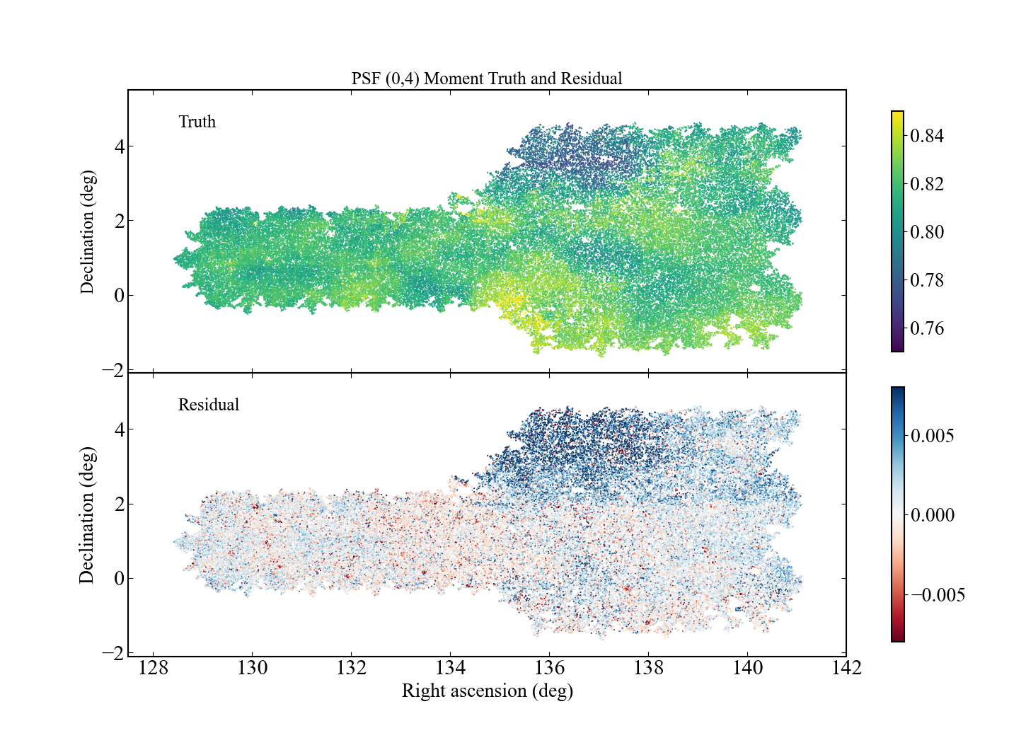
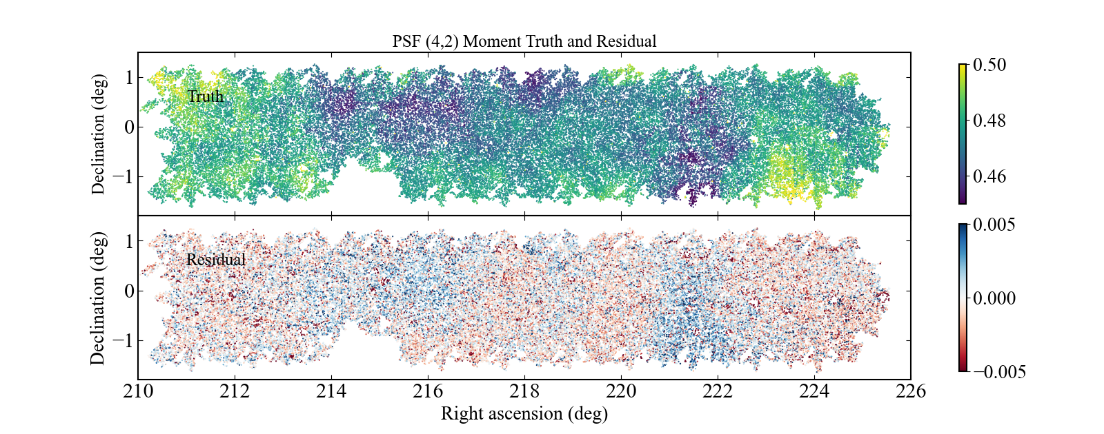
A.2 Comparison between Piff and PSFEx in RC2
In Figure 15, we show an apples-to-apples comparison between Piff and PSFEx on the RC2 dataset. This is in addition to the comparison made in Section 3.3. Due to their settings, PSFEx and Piff have opposite signs in many key moments for the weak lensing systematics. However, PSFEx shows lower moment residuals compared to Piff. This further motivates the development and optimization of Piff, which when properly tuned should improve in performance.
Appendix B Shapelet-Moment Relation

In Section 4.3, we explained that the key to changing the PSF moments through a shapelet decomposition is to compute the Jacobian matrix using Eq. (20). In Fig. 16, we show an example of the Jacobian matrix for PSF higher moment errors with respect to the shapelet modes for a Kolmogorov PSF. There is a block diagonal structure that shows the PSF second moments depend on the to shapelet modes. The PSF third moments depend on the to shapelet modes. The PSF fourth moments depend not only on the to shapelet modes, but also on the shapelet modes that determine the second moments. This means that the nth PSF higher moments basis can be approximately decomposed into shapelets components with the same order .
Appendix C Symmetry in the response to PSF higher moments
In Fig. 6, it is clear that the shear response to the PSF higher moments exhibits symmetries among the different higher moments. In this section, we explore and explain this symmetry. We start by proposing four lemmas, and derive the symmetry of the shear response based on these four lemmas.
Lemma 1: For any two PSF modeling residual basis functions and such that can be obtained by rotating by , the corresponding shear biases and satisfy the following constraint:
| (33) |
Note that this Lemma is also the basis for the fact that a 90 rotated galaxy pair has an average shape of , a fact that we use in the single galaxy simulations. We also stress that the in this section is a functional basis of the higher moments error (see Fig. 5 for examples), different from the moment biases elsewhere.
Lemma 2: The PSF modeling residual function has the form
| if p is even | (34) | ||||
| if p is odd. | (35) |
This is due to the symmetry (asymmetry) in the even (odd) functions used in the moment measurement.
Lemma 3: Similar to Lemma 2, the PSF modeling residual function has the form:
| if q is even | (36) | ||||
| if q is odd. | (37) |
Lemma 4: For any and , the PSF modeling residual function satisfies the relationship
| (38) |
This is easily proved by substituting for and vice versa.
With these lemmas, we can identify symmetry relationships between different moments, as long as the moment responses are rotations of each other. But first, we must define the rotation operators and ,
- •
– a function that rotates the moment response by deg clockwise.
- •
– a function that rotates the moment response by counter-clockwise.
Fig. 6 shows that the symmetry between results for different moments depends on the parity of the moment index and . Therefore, we consider four scenarios with different parities.
Case 1: If both and are even:
| (39) | ||||
The first two steps use Lemma 4 and Lemma 3, respectively. The last step relies on the definition of . Using Lemma 1 on the very left-hand-side (LHS) and very right-hand-size (RHS) of this equation, we infer that , which is consistent with the results for in Fig. 6. This case also implies that for even values of , must be 0, as is seen for the case in Fig. 6.
Case 2: If is even and is odd:
| (40) | ||||
The first two steps utilize Lemma 4 and Lemma 2, respectively. The last step relies on the definition of . With Lemma 1 applied to the very LHS and RHS, we infer that for this case. This finding is consistent with the results for and in Fig. 6.
Case 3: If is odd and is even, the only difference from Case 2 is to flip instead of in the second step:
| (41) | ||||
The first two steps utilize Lemma 4 and Lemma 3. The last step relies on the definition of . With Lemma 1 applied to the very LHS and RHS, we infer that .
Case 4: If both and are odd:
| (42) | ||||
The first two steps use Lemma 4 and Lemma 3. The last step relies on the definition of . Applying Lemma 1 to the very LHS and RHS, we infer that . This finding is consistent with the results for in Fig. 6.
In conclusion, only when both and are odd will we get . Otherwise, , implying that pairings with even values of produce zero shear bias. As described above, these symmetry patterns are displayed in Fig. 6. While not shown in the plot, we have explicitly confirmed that the above conclusions apply to the 5th and 6th moments as well, and they should hold beyond that as well.
Appendix D Generating the Gaussian Random Fields
In Fig. 17, we show the correlation functions of the PSF higher moment residual maps, described in Eq. (15), of the two groups of moments that determine the additive shear biases, defined in Section 5.2. These two groups of PSF higher moments are later used to propagate PSF higher moment error to the cosmoDC2 galaxies in Section 5.3. The blue dots are the measurements based on the HSC bright stars and PSFEx in Section 3.3.
We have devised empirical fitting formulae to describe the measurements of the correlation functions shown as blue dots. We fit the ‘ group’ correlation functions with a power-arctan function,
| (43) |
This model is chosen because the correlation function takes the form of a power law on small scales (or a linear function when plotted on a log-log plot), and then rapidly drops to zero. The part in the parenthesis is designed to produce the rapid drop to zero on scales beyond , a scale that is comparable to the size of the Subaru FOV. For the ‘ group’ correlation functions, we use a power law,
| (44) |
as correlation functions in the ‘ group’ moments are visually consistent with a power law.
Since the cosmoDC2 catalog has an area larger than any field in the HSC data we measure, we need to generate artificial PSF moment residual maps to cover the cosmoDC2 area. We convert the above fitting functions to angular power spectra by carrying out a Hankel transform, using SkyLens1414 14 https://github.com/sukhdeep2/Skylens_public/tree/imaster_paper/ (Singh 2021), and use the power spectra to generate artificial Gaussian Random Fields (GRF) using Healpy (Zonca et al. 2019; Górski et al. 2005). To ensure the integration is stable and bug-free, we do a round-trip transformation test, where we transform the power spectrum back to real space, shown in the orange curves in Fig. 17. The round-trip transformations match the original data well in all cases, as a validation of the fitting function and the numerical accuracy of these transformations. The GRF is generated on the HEALPix sphere with , with a pixel size arcmin. We measure the correlation function of the GRF, shown as the green curves in Fig. 17. Except for the angular bins that are below the resolution of the HEALPix grid, the GRF is shown to match the original field well in terms of the two-point statistics.