Testing Born-Infeld $f(T)$ teleparallel gravity through Sgr A^⋆ observations

Black holes can be currently considered the leading astrophysical laboratories for testing General Relativity (GR) as well as any theory of modified and quantum gravity. They allow tests in strong field regime and potentially are one of the main tools to discriminate among concurring theories of gravity. In particular, recent advances in optical, radio, X-ray and gravitational wave astronomy Abbott:2016blz; EventHorizonTelescope:2019dse; EventHorizonTelescope:2019uob; EHT2022-1; EHT2022-2; EHT2022-3 have directly confirmed the presence of supermassive black holes in the galactic centers of giant elliptical and spiral galaxies, as well as small astrophysical black holes of medium and stellar sizes. Due to the observations of the first radio images of the supermassive black hole at the center of the M87* galaxy, by Event Horizon Telescope (EHT) collaboration, black hole shadows have become a very useful tool to test GR and examine whether possible deviations from it are possible CANTATA:2021ktz. In such studies, one first calculates the shadows of various black hole solutions Shaikh:2019fpu; Wei:2019pjf; Moffat:2019uxp; Firouzjaee:2019aij; Banerjee:2019cjk; Long:2019nox; Zhu:2019ura; Konoplya:2019goy; Contreras:2019cmf; Li:2020drn; Kumar:2020pol; Pantig:2020uhp; Xavier:2020egv; Guo:2020zmf; Roy:2020dyy; Jin:2020emq; Islam:2020xmy; Chen:2020aix; Jusufi:2020zln and then confronts them with the M87* data Davoudiasl:2019nlo; Bar:2019pnz; Jusufi:2019nrn; Sau:2020xau; Belhaj:2020rdb; Kumar:2020yem; Zeng:2020vsj; Saurabh:2020zqg; Bambi:2019tjh; Vagnozzi:2019apd; Haroon:2019new; Shaikh:2019hbm; Cunha:2019ikd; Banerjee:2019nnj; Feng:2019zzn; Li:2019lsm; Allahyari:2019jqz; Rummel:2019ads; Vagnozzi:2020quf; Chang:2020lmg; Kruglov:2020tes; Ghosh:2020tdu; Psaltis:2020lvx; Hu:2020usx; Li:2021mzq; Addazi; Felix1; Felix2; Felix3.

GR predicts that the unique astrophysically viable asymptotically flat black hole solution is only described by its mass, angular momentum and charge. In astrophysics, the charge is usually very small so it does not play any role. Further, if one only takes spherical symmetry, the solution is just described by its mass and, thus, the Schwarzschild solution. If one modifies GR, then, there could be more asymptotically flat spherically symmetric black hole solutions. There are several ways of modifying GR Capozziello:2011et; Faraoni. One interesting approach is the so-called teleparallel gravity when curvature is zero but torsion is non-zero Bahamonde:2021gfp; Aldrovandi:2013wha; Cai; Krssak:2018ywd (still the compatibility condition holds $\accentset{\circ}{\nabla}_{\alpha}g_{\mu\nu}=0$). It turns out that there is a theory which is equivalent to GR (having the same predictions and classical field equations), which is known as the teleparallel equivalent of GR (see Aldrovandi:2013wha). The action of this theory is built from the torsion scalar $T$ which is constructed by contraction of torsion tensor with some particular coefficients in front. This scalar $T$ differs by a boundary term with respect to the Levi-Civita Ricci scalar $\mathring{R}$. If one starts from this theory, one can modify its action and formulate modified teleparallel theories of gravity (see Bahamonde:2021gfp for a comprehensive review about them). For example, one can formulate modified theories by having the three scalars constructed by the torsion tensor Hayashi:1979qx; Bahamonde:2017wwk, or by introducing scalar fields, which are the so-called scalar-torsion theories Geng:2011aj; Gonzalez:2015sha; Bahamonde:2019shr; Hohmann:2018ijr; Hohmann:2018vle; Hohmann:2018dqh; Hohmann:2018rwf, or by including the boundary term $B$ Bahamonde:2015zma; Bahamonde:2019jkf; Bahamonde:2020bbc; Escamilla-Rivera:2019ulu; Caruana:2020szx, or even by considering other scalars such as the teleparallel Gauss-Bonnet Kofinas:2014owa; Bahamonde:2016kba; Capozziello:2016eaz. Due to the nature of the torsion tensor, it is much simpler than in the Riemannian case to construct theories with second order field equations. The covariant formulation of these theories were already developed in Krssak:2015oua; Golovnev:2017dox; Krssak:2018ywd.

One famous modification in teleparallel gravity is known as $f(T)$ that it is achieved by upgrading the torsion scalar to any arbitrary function Ferraro:2008ey; Ferraro:2006jd; Bengochea:2008gz; Krssak:2015oua. This theory is usually formulated with tetrads and a spin connection which is always pure gauge. This means that it is always possible to choose a specific gauge such that the spin connection vanishes. Further, this theory contains symmetric and antisymmetric field equations. If one imposes that both the metric and the connection respects spherical symmetry, then the two most general tetrads (in the Weitzenböck gauge) Hohmann:2019nat that solve the antisymmetric field equations for $f(T)$ were obtained in Bahamonde:2021srr. The first one is real and so far, there are not non-trivial exact black hole solutions (only perturbed ones) Bahamonde:2019zea; Ruggiero:2015oka; DeBenedictis:2016aze; Bahamonde:2020vpb; Golovnev:2021htv; Pfeifer:2021njm. Further, using numerical and a dynamical approach, it has been found that the real tetrad contains a regular black hole solution in $f(T)$ Born-Infeld gravity Bohmer:2020jrh; Bohmer:2019vff. On the other hand, it has been recently found that for the complex tetrad, there are two exact asymptotically flat black hole solutions for two different theories, a Born-Infeld $f(T)$ and a more complicated one given by non-trivial modifications of GR Bahamonde:2021srr. These two exact black solutions represent the first non-trivial ones in the literature of teleparallel gravity. In the context of scalar-torsion theories, recently, new exact scalarized black hole solutions were obtained in Bahamonde:2022lvh.

Our aim is to study the astrophysical properties of the exact black hole solution found in Born-Infeld $f(T)$ gravity and use data to constrain its parameter. This particular theory also has the interesting feature that it can describe inflation without introducing a scalar field. This paper is organized as follows. In Section II, we briefly review teleparallel gravity and exact Born-Infeld solution reported recently in Bahamonde:2021srr. In Section III, we study the shadow images in Born-Infeld $f(T)$ gravity. In Section IV, we constrain the parameter of the solutions using the motion of the S2 star orbit. In Section V, we investigate the deflection angle of light in the weak gravity regime. Finally in Section VI, we comment on our results. Throughout this paper, Latin indices refer to tangent space and the Greek indices label coordinates on spacetime. Overcircles quantities are computed from the Levi-Civita connection (Riemannian quantities), we assume the metric signature $(+---)$ and natural units $c=G=1$.

In what follows we provide a brief review on teleparallel gravity and $f(T)$ gravity. These theories are constructed in a manifold which is globally flat and assumes the compatibility condition. Hence, torsion is the field strength tensor of the theory which is the responsible of gravity. Its formulation is usually built from tetrads $e^{a}{}_{\mu}$ (orthonormal basis on tangent space) and a purely-gauge spin connection $w^{a}{}_{b\mu}$ (see Bahamonde:2021gfp for more details about these theories). According to this picture, the metric tensor can be expressed in terms of the tetrad field terms of the following equation

$$g_{\mu\nu}=\eta_{ab}e^{a}{}_{\mu}e^{b}{}_{\nu}\ ,$$

(1)

in which $\eta_{ab}=\text{diag}(1,-1,-1,-1)$ is the Minkowski metric. Using them, we define the torsion tensor as

$$T^{\rho}{}_{\mu\nu}=e_{a}{}^{\rho}\left(\partial_{\mu}e^{a}{}_{\nu}-\partial_{\nu}e^{a}{}_{\mu}+\omega^{a}{}_{b\mu}e^{b}{}_{\nu}-\omega^{a}{}_{b\nu}e^{b}{}_{\mu}\right)\,.$$

(2)

It can be shown that the torsion tensor is invariant under local Lorentz transformations if one simultaneously transforms the tetrad and spin connection. Since the spin connection is purely-gauge as $\omega^{a}{}_{b\mu}=\Lambda^{a}{}_{c}\partial_{\mu}(\Lambda^{-1})^{c}{}_{b}\,$, one can always choose a gauge (known as the Weitzenböck gauge) such that it vanishes.

One of the most remarkable results in these theories is that there is an equivalent description of GR but based purely on torsion, the so-called teleparallel equivalent of GR which is built from the action

$${\cal{S}}=\frac{1}{16\pi}\int{T\,e\,d^{4}x}+{\cal{S}}_{M}\ ,$$

(3)

with $e=\text{det}(e^{a}{}_{\mu})=\sqrt{-\text{det}(g_{\mu\nu})}$, ${\cal{S}}_{M}$ represents the action for the matter fields that it is usually assumed to be coupled minimally to the metric, and $T$ is known as the torsion scalar which is defined as

$$T=\frac{1}{4}T^{\rho\sigma\mu}T_{\rho\sigma\mu}+\frac{1}{2}T^{\mu\sigma\rho}T_{\rho\sigma\mu}-T^{\rho}{}_{\rho\sigma}T^{\mu}{}_{\mu}{}^{\sigma}\,.$$

(4)

This teleparallel scalar is connected to the Riemannian Ricci scalar as $\mathring{R}=-T+\tfrac{2}{e}\partial_{\mu}(eT^{\lambda}{}_{\lambda}{}^{\mu})$. Clearly, (3) provides the same equations as the Einstein’s field equations since $T$ differs by a boundary term to $\accentset{\circ}{R}$ and appears linearly in the action. One can then modify this action to construct modified teleparallel theories of gravity. One of the most famous ones is the one when one upgrades $T$ by an arbitrary and differentiable function of it, namely

$${\cal{S}}=\frac{1}{16\pi}\int{f(T)\,e\,d^{4}x}+{\cal{S}}_{M}\,.$$

(5)

If we vary this action with respect to $e^{a}{}_{\mu}$, one finds that the vacuum field equations in the Weitzenböck gauge are

$\displaystyle(\partial_{\mu}f_{T})S_{\nu}{}^{\mu\lambda}+e^{-1}e^{a}{}_{\nu}\partial_{\mu}(eS_{a}{}^{\mu\lambda})f_{T}-f_{T}T^{\sigma}{}_{\mu\nu}S_{\sigma}{}^{\lambda\mu}-\frac{1}{2}f\delta_{\nu}^{\lambda}=0$

where $f_{T}=df/dT$ and we defined the superpotential as

$$S_{\rho\mu\nu}=\frac{1}{2}\left(T_{\nu\mu\rho}+T_{\rho\mu\nu}-T_{\mu\nu\rho}\right)-g_{\rho\mu}T^{\sigma}{}_{\sigma\nu}+g_{\rho\nu}T^{\sigma}{}_{\sigma\mu}\,.$$

(6)

The field equations (II) have symmetric and antisymmetric contributions. The antisymmetric part of the field equations in spherical symmetry has two branches, one given by a real tetrad and another one by a complex one. Recently, two exact black hole solutions in $f(T)$ teleparallel gravity were reported by Bahamonde et al. Bahamonde:2021srr. These solutions were found in the second branch with tetrad field being Bahamonde:2021srr

$\displaystyle e^{a}{}_{\mu}$

$\displaystyle=$

$\displaystyle\left(\begin{array}[]{cccc}0&i\mathcal{B}(r)&0&0\\ i\mathcal{A}(r)\sin\theta\cos\phi&0&-r\sin\phi&-r\sin\theta\cos\theta\cos\phi\\ i\mathcal{A}(r)\sin\theta\sin\phi&0&r\cos\phi&-r\sin\theta\cos\theta\sin\phi\\ i\mathcal{A}(r)\cos\theta&0&0&r\sin^{2}\theta\\ \end{array}\right)\,,$

which reproduces the spherically symmetric metric

$\displaystyle ds^{2}$

$\displaystyle=$

$\displaystyle\mathcal{A}(r)^{2}dt^{2}-\mathcal{B}(r)^{2}dr^{2}-r^{2}d\Omega^{2}\,,$

(12)

where $d\Omega^{2}=d\theta^{2}+\sin^{2}\theta d\phi^{2}$ is the line element of a two dimensional unit sphere. The torsion tensor for this tetrad is spherically symmetric (and real) and the torsion scalar behaves as

$\displaystyle T$

$\displaystyle=$

$\displaystyle\frac{2}{r^{2}\mathcal{B}^{2}\mathcal{A}}\left(\left(\mathcal{B}^{2}+1\right)\mathcal{A}+2r\mathcal{A}^{\prime}\right)\,.$

(13)

Our main aim is to investigate the phenomenology of this new exact black hole solution. The exact solution is based on a theory motivated from Born-Infeld electromagnetism, which has the following form of the function

$$f(T)=\lambda\Big(\sqrt{1+\frac{2T}{\lambda}}-1\Big)\,,$$

(14)

with $\lambda$ being the so-called Born-Infeld parameter. It is interesting to mention that Born-Infeld $f(T)$ gravity was the first modified teleparallel gravity studied in the context of inflation Ferraro:2008ey. If one assumes that $T/\lambda\ll 1$, then $f(T)=T-T^{2}/(2\lambda)+\mathcal{O}(1/\lambda^{2})$ which behaves as TEGR (or GR) and a torsion-squared correction. For this theory and the tetrad (II), there is the following exact spherically symmetric solution Bahamonde:2021srr

$\displaystyle ds^{2}=\frac{a_{1}^{2}}{r}\Big[\sqrt{\lambda}(a_{0}\lambda+r)-2\tan^{-1}\left(\frac{\sqrt{\lambda}r}{2}\right)\Big]dt^{2}-\frac{\lambda^{5/2}r^{5}}{(4+r^{2}\lambda)^{2}}\Big[\sqrt{\lambda}(a_{0}\lambda+r)-2\tan^{-1}\left(\frac{\sqrt{\lambda}r}{2}\right)\Big]^{-1}dr^{2}-r^{2}d\Omega^{2}\,,$

(15)

where $a_{0},a_{1}$ are integration constants. In order to obtain an asymptotically flat spacetime we require that $a_{1}^{2}=1/\sqrt{\lambda}$. Further, to have a smooth transition from the Schwarzschild solution of TEGR ($\lambda\rightarrow\infty$) one needs to set $a_{0}=-2M/\lambda$. Doing so, and by introducing the parameter

$\displaystyle\alpha=\frac{1}{\lambda}$

(16)

we obtain that the metric becomes

$\displaystyle ds^{2}=\Big[1-\frac{2M}{r}-\frac{2\sqrt{\alpha}}{r}\tan^{-1}\left(\frac{r}{2\sqrt{\alpha}}\right)\Big]dt^{2}-\frac{\alpha^{-5/2}r^{5}}{(4+r^{2}/\alpha)^{2}}\Big[1-\frac{2M}{r}-\frac{2\sqrt{\alpha}}{r}\tan^{-1}\left(\frac{r}{2\sqrt{\alpha}}\right)\Big]^{-1}dr^{2}-r^{2}d\Omega^{2}\,.$

(17)

Thus, smaller values of $\alpha$ would mean that the deviation from GR would be smaller. Let us compute the ADM mass which coincides with the Komar mass in our case and it is defined as

$\displaystyle\mathcal{M}=\lim_{r\to\infty}\frac{r}{2}\left(1-g^{ab}(\partial_{a}r)(\partial_{b}r)\right)=M+\frac{\pi\sqrt{\alpha}}{2}\,.$

(18)

One can notice that the ADM mass $\mathcal{M}$ is shifted by $\frac{\pi\sqrt{\alpha}}{2}$ with respect to the mass parameter $M$.

If we now assume that $T/\lambda\ll 1$ and we expand the metric up to $\mathcal{O}(\alpha^{2})$, we notice that the metric becomes

$\displaystyle ds^{2}=\Big[1-\frac{2M}{r}+\frac{4\,\alpha}{r^{2}}-\frac{\pi\sqrt{\alpha}}{r}\Big]dt^{2}-\Big[1-\frac{2M}{r}-\frac{16M\,\alpha}{r^{3}}+\frac{12\alpha}{r^{2}}-\frac{\pi\sqrt{\alpha}}{r}\Big]^{-1}dr^{2}-r^{2}d\Omega^{2}+\mathcal{O}(\alpha^{2})\,,$

(19)

where one can see that this solution behaves as Schwarzschild in addition to some corrections. It is known that this exact solution contains an event horizon as reported in Bahamonde:2021srr.

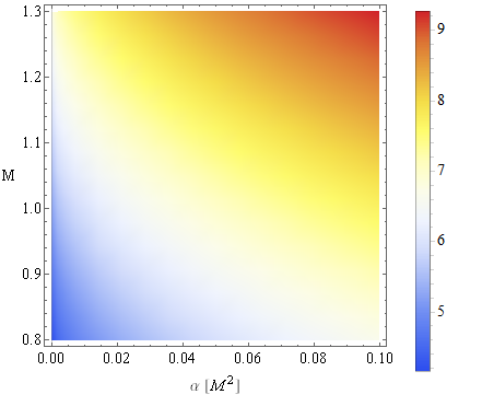
We can use the two impact parameters $\xi$ and $\eta$ in order to analyze the motion of photons around the black hole. Since we are interested to explore the possible deviations from GR encoded in the parameter $\alpha$ we need to use the conditions for unstable orbit. As we know, in the observer’s sky, we can observe the black hole shadow due to the fact that some of the scattered photons escape from the black hole while some photons are captured by the black hole. These unstable circular photon orbits can be obtained by applying the following conditions:

$$V_{\text{eff}}(r)=0\,,\quad\frac{dV_{\text{eff}}}{dr}=0\,,\quad\frac{d^{2}V_{\text{eff}}}{dr^{2}}\leq 0\,.$$

(27)

Using Eqs. (22) and (24) it is easy to combine $V_{\text{eff}}$ and $R(r)$. If we express the above conditions in terms of $R(r)$ we obtain:

$$R(r)=0\,,\quad\frac{dR(r)}{dr}=0\,,\quad\frac{d^{2}R(r)}{dr^{2}}>0\,.$$

(28)

The radius of the photon sphere can be used to find the size of black hole shadow. In order to describe the shadow as seen by large distances, one introduces the two celestial coordinates $X$ and $Y$ Chandra, namely

	$\displaystyle X$	$\displaystyle=\lim_{r_{*}\to\infty}\left(-r_{*}^{2}\sin\theta_{0}\frac{d\phi}{dr}\right)\,,$		(29)
	$\displaystyle Y$	$\displaystyle=\lim_{r_{*}\to\infty}r_{*}^{2}\frac{d\theta}{dr}\,,$		(30)

with $r_{*}$ the distance between the black hole and the observer, and $\theta_{0}$ the inclination angle between the observer’s line of sight and the black hole rotational axis.

Using the geodesics equations we finally obtain

	$\displaystyle X=-\xi(r_{\rm ph})\csc\theta_{0}\,,$		(31)
	$\displaystyle Y=\sqrt{\eta(r_{\rm ph})-\xi^{2}(r_{\rm ph})\cot^{2}\theta_{0}}\,,$		(32)

and thus we have $X^{2}+Y^{2}=\xi^{2}(r_{\rm ph})+\eta(r_{\rm ph})$. Hence, the shadow radius $R_{\rm sh}$ can finally be found as

$$R_{\rm sh}(r_{\rm ph})=\sqrt{\xi^{2}(r_{\rm ph})+\eta(r_{\rm ph})}=\frac{r_{\rm ph}}{\mathcal{A}(r_{\rm ph})}\,.$$

(33)

The angular diameter of the shadow can be defined as

$\displaystyle\theta_{\rm sh}=\frac{2\,R_{\rm sh}M}{D}\,,$

(34)

where $D$ is the distance from the black hole and $M$ is the black hole mass. In Fig 1, we display the shadow radius of the black hole in Born-Infeld $f(T)$ gravity as a function of the parameter $\alpha$. We find that the shadow radius increases with the increase of $\alpha$.

We can see that the event horizon radius is expected to increase due to parameter $\alpha$. We close this section by considering the scenario where the black hole is surrounded by an infalling/radiating accretion flow. Via this simple model, one can extract valuable information about the intensity of the radiation which can be detected by a distant observer. In order to achieve this we need to estimate the specific intensity at the observed photon frequency $\nu_{\text{obs}}$ at the point $(X,Y)$ of the observer’s image Narayan:2019imo; Saurabh:2020zqg; Jusufi:2020zln; Zeng:2020dco; Falcke:1999pj; Bambi:2013nla

$\displaystyle I_{\rm obs}(\nu_{\rm obs},X,Y)=\int_{\gamma}\mathrm{g}^{3}j(\nu_{e})dl_{\text{prop}}\,.$

(35)

We consider a freely-falling gas dropped from rest at infinity with $E=1$, which has the following four-velocity

$\displaystyle u^{\mu}_{e}=\Big(\frac{1}{\mathcal{A}^{2}(r)},-\frac{1}{\mathcal{A}(r)\mathcal{B}(r)}\sqrt{1-\mathcal{A}^{2}(r)},0,0\Big)\,.$

(36)

In addition we need to use the condition $p_{\mu}p^{\mu}=0$, from which one can easily obtain

$\displaystyle\frac{p^{r}}{p^{t}}=\pm\frac{\mathcal{A}^{2}(r)}{\mathcal{B}(r)}\sqrt{\bigg(\frac{1}{\mathcal{A}^{2}(r)}-\frac{b^{2}}{r^{2}}\bigg)}\,,$

(37)

with $b$ being the impact parameter. It is important to mention here that sign $+(-)$ describes the case when the photon approaches (or draws away) from the black hole. The redshift function $z$ can be calculated using Narayan:2019imo; Saurabh:2020zqg; Jusufi:2020zln; Zeng:2020dco; Falcke:1999pj; Bambi:2013nla

$\displaystyle z=\frac{p_{\mu}u_{\rm obs}^{\mu}}{p_{\nu}u_{e}^{\nu}}\,,$

(38)

with $u_{\rm obs}^{\mu}$ the 4-velocity of the observer. For the specific emissivity we assume a simple model in which the emission is monochromatic, with emitter’s-rest frame frequency $\nu_{\star}$, and the emission has a $1/r^{2}$ radial profile:

$\displaystyle j(\nu_{e})\propto\frac{\delta_{D}(\nu_{e}-\nu_{\star})}{r^{2}}\,,$

(39)

where $\delta_{D}$ denotes the Dirac delta function. The accretion flow has spherically symmetry and it can be described as an optically-thin disk region around the black hole. Expressing the proper length in terms of radial coordinate for observed flux, we find

$\displaystyle F_{\rm obs}(X,Y)\propto-\int_{\gamma}\frac{z^{3}\,p_{t}}{r^{2}p^{r}}dr.$

(40)

In the next section we will constrain the parameter $\alpha$ and use its best fit value to plot the shadow images for the Sgr A^⋆ black hole.

Let us now focus on the most important aspect of the present work which is to constrain the parameter of the theory and test this solution with observations from the shadow of the Sgr A^⋆ central black hole. For the distance we shall assume the distance $D=8.3$ kpc, while for the black hole mass we can take $M=4.1\times 10^{6}$ M$\textsubscript{$\odot$}.$ Our strategy is to first constrain $\alpha$ using the motion of the S2 star orbit (see, the data Gillessen:2009ht; GRAVITY:2018ofz) and then construct the specific shadow images within the range of validity of the observations and more specifically, its best fitting value. To study the motion of a test particle using the $f(T)$ solution, without loss of generality, we can take the equatorial plane with $(\theta=\pi/2,~\dot{\theta}=0)$, and then having in mind that there are two constants of motion (namely the total energy $E$ and the total angular momentum $L$ of the S2 star) which are given by

$$\dot{t}=\frac{E}{\mathcal{A}^{2}(r)}\,,\quad\dot{\phi}=\frac{L}{r^{2}},$$

(41)

where dots refer differentiation with respect to the arc-length parameter $\delta$. One can also find that the radial equation of motion for the particle (S2 star in our case) is given by Do:2019txf; Becerra-Vergara:2020xoj; Nampalliwar:2021tyz

$$\ddot{r}=-\dfrac{1}{2\mathcal{B}^{2}(r)}\left[\frac{d\mathcal{A}^{2}(r)}{dr}\ \dot{t}^{2}-\frac{d\mathcal{B}^{2}(r)}{dr}\ \dot{r}^{2}-2r\dot{\phi}^{2}\right]\,.$$

(42)

The real position is given by the Cartesian coordinates $(x,y,z)$, along with the corresponding velocity components $(v_{x},v_{y},v_{z})$. From the Cartesian coordinates we can find the coordinates in spherical coordinates in the equatorial plane easily using

$\displaystyle x$

$\displaystyle=r\cos\phi\,,\quad y=r\sin\phi\,,\quad z=0\,,$

(43)

with the corresponding three-velocities given by

$$v_{x}=v_{r}\cos\phi-rv_{\phi}\sin\phi\,,\quad v_{y}=v_{r}\sin\phi+rv_{\phi}\cos\phi\,,\quad v_{z}=0\,.$$

(44)

During the numerical analyses, from the observers point of view, we need to work with the apparent orbit which has the coordinates $(\mathcal{X},\mathcal{Y},\mathcal{Z})$ related to the real orbit given by $(x,y,z)$ using 13

$\displaystyle\mathcal{X}=xB+yG\,,\quad\mathcal{Y}=xA+yF\,,\quad\mathcal{Z}=xC+yF\,,$

(45)

whereas for the apparent components of the velocity and the real component of the velocity we have the relations 13

$\displaystyle\mathcal{V}_{X}=v_{x}B+v_{y}G\,,\quad\mathcal{V}_{Y}=v_{x}A+v_{y}F\,,\quad\mathcal{V}_{Z}=v_{x}C+v_{y}F\,,$

(46)

in which we defined 13

	$\displaystyle B$	$\displaystyle=$	$\displaystyle\sin\Omega\cos\omega+\cos\Omega\sin\omega\cos i\,,$		(47)
	$\displaystyle G$	$\displaystyle=$	$\displaystyle-\sin\Omega\sin\omega+\cos\Omega\cos\omega\cos i\,,$		(48)
	$\displaystyle A$	$\displaystyle=$	$\displaystyle\cos\Omega\cos\omega-\sin\Omega\sin\omega\cos i\,,$		(49)
	$\displaystyle F$	$\displaystyle=$	$\displaystyle-\cos\Omega\sin\omega-\sin\Omega\cos\omega\cos i\,,$		(50)
	$\displaystyle C$	$\displaystyle=$	$\displaystyle\sin\omega\sin i\,,$		(51)
	$\displaystyle F$	$\displaystyle=$	$\displaystyle\cos\omega\sin i\,.$		(52)

Note here the following important quantities: $\omega$, $i$, and $\Omega$ which are the argument of pericenter, the inclination between the real orbit and the observation plane, and the ascending node angle, respectively. Recently, the Gravity Collaboration measured for the first time the orbital precession of S2, and constrained its departure from the one predicted in GR whose best fit value is $f_{SP}=1.10\pm 0.19$ GRAVITY:2020gka. Here a value $f_{SP}=0$ recovers Newtonian’s gravity and $f_{SP}=1$ which is consistent with GR. The result clearly shows that GR is consistent with observations. In the present work, we would like to test a possible deviations from GR using the modified gravity $f(T)$ gravity solutions. One must relay on the numerical analyses to obtain the equations of motion for the orbit. We are going to use the Bayesian theorem with the likelihood function with the posterior probability density with the likelihood function is given by

$\displaystyle\ln\mathcal{L}(O|P)=-\frac{1}{2}\sum_{i=1}^{N}\left[\frac{\left(X_{\textrm{ obs},i}-X_{\textrm{mod},i}\right)^{2}}{\sigma_{\textrm{obs},i}^{2}}\right]-\frac{1}{2}\sum_{i=1}^{N}\left[\frac{\left(Y_{\textrm{obs},i}-Y_{\textrm{mod},i}\right)^{2}}{\sigma_{\textrm{obs},i}^{2}}\right]\,,$

(53)

where the two observed and theoretical quantities are noted as $(X_{\rm obs},Y_{\rm obs})$, and $(X_{mod},Y_{mod})$ (see, GRAVITY:2018ofz; Do:2019txf). In order to find the best-fit values we use the Monte-Carlo-Markov Chains analysis. For the central mass object we take $4.1\times 10^{6}M_{\odot}$ along with the uniform priors $\alpha/M^{2}\in[0,1]$ for the Solution 2, respectively. In Fig. 2, we present the region of the parameter space in agreement with S2 star data. Concerning the $\alpha$ parameter, in which we are interested in this manuscript, the best fit within 1$\sigma$ confidence are given in Table I.

Within $1\sigma$ we found an upper bound $0\leq\alpha/M^{2}\leq 6\times 10^{-4}$ for the Born-Infeld $f(T)$ gravity. Using the constraints we have presented the shadow of Sgr A^⋆ black hole as shown in Fig. 3. For the angular diameter we have found $52.530\,\mu$arcsec. Using the recent result reported for Sgr A^⋆ given by $(51.8\pm 2.3)\mu$arcsec EHT2022-1; EHT2022-2; EHT2022-3 we conclude that the angular diameter of the Born-Infeld $f(T)$ gravity is consistent with the observation and could not be distinguished from the Schwarzschild black hole in GR by the present technology. From the shadow images given in Fig. 3, one can observe the characteristic photon rings and also an interesting fact that the intensities of the electromagnetic radiation are small in Born-Infeld $f(T)$ gravity models compared to Schwarzschild black hole.

In this final section, we will proceed to elaborate the gravitational lensing effect in weak gravity regime in $f(T)$ gravity models using the optical geometry. For the general case, in the equatorial plane by letting $ds^{2}=0$, we find the optical metric

$\displaystyle dt^{2}=\frac{\mathcal{B}^{2}(r)dr^{2}}{\mathcal{A}^{2}(r)}+\frac{r^{2}d\phi^{2}}{\mathcal{A}^{2}(r)}.$

(54)

To simplify further the work, we can write the optical metric in approximated form in leading order in $\alpha$, in the equatorial plane, given by (see the expanded metric in (19))

$$dt^{2}\simeq\frac{dr^{2}}{\left[1-\frac{2M}{r}+\frac{4\,\alpha}{r^{2}}-\frac{\pi\sqrt{\alpha}}{r}\right]\left[1-\frac{2M}{r}+\frac{12\,\alpha}{r^{2}}-\frac{\pi\sqrt{\alpha}}{r}\right]}+\frac{r^{2}d\phi^{2}}{1-\frac{2M}{r}+\frac{4\,\alpha}{r^{2}}-\frac{\pi\sqrt{\alpha}}{r}}+\mathcal{O}(\alpha^{2})$$

(55)

In what follows we shall apply the optical geometry by applying the Gauss-Bonnet theorem to compute the deflection angle of light, which can be summarised as follows:
Theorem Let $\mathcal{D}_{R}$ be a non-singular domain outside the light ray with boundaries $\partial\mathcal{D}_{R}=\gamma_{g^{(\rm op)}}\cup C_{R}$, of an oriented two-dimensional surface $S$ with the optical metric $g^{(\rm op)}$. Moreover let $\mathcal{K}$ and $\kappa$ be the Gaussian optical curvature and the geodesic curvature associated to the optical geometry. Under this construction the Gauss-Bonnet theorem can be written as follows Gibbons

$$\int\limits_{\mathcal{D}_{R}}\mathcal{K}\,dS+\oint\limits_{\partial\mathcal{A}_{R}}\kappa\,dt+\sum_{k}\theta_{k}=2\pi\chi(\mathcal{D}_{R})\,.$$

(56)

In this equation $\theta_{k}$ stands for the exterior angle at the $k^{\rm th}$ vertex. We chose the regular domain to be outside of the light ray, say in the $(r,\phi)$ optical plane, this means that the domain has the topology of disc having the Euler characteristic number $\chi(\mathcal{D}_{R})=1$. Furthermore we need to compute two important quantities: the Gaussian optical curvature and the geodesic curvature. Let us first focus on the Gaussian optical curvature $\mathcal{K}$ which in leading order terms gives

$\displaystyle\mathcal{K}$

$\displaystyle\simeq$

$\displaystyle-\frac{2M}{r^{3}}-\frac{\pi\sqrt{\alpha}}{r^{3}}+\mathcal{O}(\alpha^{2})\,.$

(57)

Let us now introduce a smooth curve defined as follows $\gamma:=\{t\}\to\mathcal{D}_{R}$, where the geodesic curvature can be found from Gibbons

$$\kappa=g^{(\rm op)}\,\left(\accentset{\circ}{\nabla}_{\dot{\gamma}}\dot{\gamma},\ddot{\gamma}\right),$$

(58)

having in mind the additional unit speed condition $g^{(\rm op)}(\dot{\gamma},\dot{\gamma})=1$, along with the $\ddot{\gamma}$ being the unit acceleration vector. In the large limit, but finite radial distance $r\equiv R\rightarrow\infty$, we have two jump angles (say at the source $\mathcal{S}$ and observer $\mathcal{O})$, which satisfy $\theta_{\mathit{O}}+\theta_{\mathit{S}}\rightarrow\pi$ Gibbons. On the other hand, for the geodesic curvature for the light ray (geodesics) we must have $\kappa(\gamma_{g^{(\rm op)}})=0$. Hence we only need to compute the contribution to the curve $C_{R}$. From the Gauss-Bonnet theorem we have

$$\lim_{R\rightarrow\infty}\int_{0}^{\pi+\hat{\alpha}_{\rm DA}}\left[\kappa\frac{dt}{d\phi}\right]_{C_{R}}d\phi=\pi-\lim_{R\rightarrow\infty}\iint\limits_{\mathcal{D}_{R}}\mathcal{K}\,dS.$$

(59)

To simplify the problem further, let us chose the black hole at the coodinate center and consequently the geodesic curvature for the curve is $C_{R}$ at the distance distance $R$ from the coordinate center. It follows that Gibbons

$$\kappa(C_{R})=|\accentset{\circ}{\nabla}_{\dot{C}_{R}}\dot{C}_{R}|.$$

(60)

We can now utilize the unit speed condition and the optical metric to show that$\lim_{R\rightarrow\infty}\kappa(C_{R})\rightarrow R^{-1}$. This shows that the optical metric is asymptotically Euclidean and therefore the deflection angle reads

$$\hat{\alpha}_{\rm DA}=-\int\limits_{0}^{\pi}\int\limits_{r(\phi)}^{\infty}\mathcal{K}dS,$$

(61)

where we have the surface element reads $dS=\sqrt{g^{(\rm op)}}drd\phi$ and the equation for the light ray $r(\phi)=b/\sin\phi$. Solving this integral we can approximate the deflection angle as

$$\hat{\alpha}_{\rm DA}=-\int\limits_{0}^{\pi}\int\limits_{\frac{\mathsf{b}}{\sin\phi}}^{\infty}\left[-\frac{2M}{r^{3}}-\frac{\pi\sqrt{\alpha}}{r^{3}}\right]dS=\frac{4M}{b}+\frac{2\pi\sqrt{\alpha}}{b}-\frac{\pi\left(3\pi^{2}+80\right)\alpha}{16\,b^{2}}+\mathcal{O}(\alpha^{2})\,.$$

(62)

From the last equation, one notices that the deflection angle is affected by the parameter $\alpha$ in leading order terms. At least mathematically, in leading order terms, it seems like we cannot distinguish the black hole in $f(T)$ gravity from the GR. Implying that the deflection angle in leading order terms expressed by the ADM mass (see Eq. (18)) is given by

$\displaystyle\hat{\alpha}_{\rm DA}=\frac{4}{b}\left(M+\frac{\pi\sqrt{\alpha}}{2}\right)-\frac{\pi\left(3\pi^{2}+80\right)\alpha}{16\,b^{2}}=\frac{4\mathcal{M}}{b}-\frac{\pi\left(3\pi^{2}+80\right)\alpha}{16\,b^{2}}+\mathcal{O}(\alpha^{2})\,.$

(63)

However from the physical point of view the ADM mass in $f(T)$ gravity, i.e. $\mathcal{M}$ is bigger compared to the mass parameter $M$, since $\alpha\geq 0$.

Of course, we see that one can go beyond the leading order term and, in that case, the second order term is a correction term proportional to $\delta\hat{\alpha}\sim-\alpha/b^{2}$, meaning that the deflection angle decreases to the $\alpha$ corrections, but the first order term which increases the mass is dominant and overall the deflection angle is expected to increase. This increase on the deflection angle explains why the intensity of electromagnetic radiation detected by a distant observer shown in Fig. 3 is smaller in $f(T)$ gravity compared to GR. The best accuracy of measuring the deflection of light by the sun is from measuring the deflection of radio waves from distant quasars using the Very Long Baseline Array (VLBA) vlbi, which achieved an accuracy of $3\times 10^{-4}$. For that we can use the leading order contribution term

$\displaystyle\frac{\delta\hat{\alpha}_{\rm DA}}{\hat{\alpha}^{GR}_{\rm DA}}=\frac{2\pi\sqrt{\alpha}/b}{4M/b}<3\times 10^{-4}.$

(64)

Assuming that light grazes the surface of the Sun with $b=6.96\times 10^{8}$ m and mass in geometric units $M=1.48$ km, we get the following interval $0\leq\alpha/M^{2}\leq 3.64\times 10^{-8}$. Where we have excluded the negative domain, we can see that the positive bound belongs to the interval obtained from the S2 star constrain given by $0\leq\alpha/M^{2}\leq 6\times 10^{-4}$.

We have used an exact solution in Born-Infeld $f(T)$ gravity and studied the phenomenological aspects using the black hole shadows and the S2 star orbit. The impact of modified gravity is encoded in the coupling parameter $\alpha$ which changes the properties of the black hole and its shadow. We used data from the orbital motion of S2 star around the Sgr A^⋆ black hole through a Monte-Carlo-Markov Chains (MCMC) analysis within $1\sigma$ we found an upper bound $0\leq\alpha/M^{2}<6\times 10^{-4}$. Using the best fit parameters we found the angular diameter $52.530\,\mu$arcsec for the shadow. Using the recent result for the angular diameter for Sgr A^⋆ reported as $(51.8\pm 2.3)\mu$arcsec EHT2022-1; EHT2022-2; EHT2022-3 we see that the angular diameter of the Born-Infeld $f(T)$ gravity is consistent with the observation and very difficult to distinguished from the Schwarzschild black hole, at least with the present data. We have also computed the deflection angle of light in the weak gravity regime and found that in leading order terms mathematically the Born-Infeld $f(T)$ gravity cannot be distinguished from the classical GR, however the ADM mass in $f(T)$ gravity is bigger due to $\alpha$ corrections and overall the deflection angle is expected to increase. This fact is in perfect agreement with our shadow image shown in Fig. 3, for Born-Infeld $f(T)$ gravity the intensity observed at infinity is smaller compared to GR. This has to do with the fact that when the deflection angle increases more photons will be captured by the black hole and the intensity will be smaller at infinity. From the weak deflection angle we obtain an upper bound given by $0\leq\alpha/M^{2}\leq 3.64\times 10^{-8}$. Finally, it should be noted that, with the improvement of the precision of measuring the shadow of black holes we should have better constraints to have a more rigorous test of modified theories of gravity.

Still there are some questions regarding the exact black hole solution that we analysed. For example, it is important to analyse its stability by performing perturbations of the tetrad. Furthermore, some other aspects that could be interesting to analyse are the predictions of the quasi-normal modes generated by having this background solution. Since the tetrad is complex, one would need to be careful on performing these perturbations carefully such that all the observables are real. Another question that could be interesting astrophysically is to analyse its viability by studying accretion disks configurations under this solution. All of these studies will be reported in forthcoming studies.

References

- (1) B. P. Abbott et al. [LIGO Scientific and Virgo Collaborations], Phys. Rev. Lett. 116, no. 6, 061102 (2016) [arXiv:1602.03837].
- (2) K. Akiyama et al. [Event Horizon Telescope], Astrophys. J. Lett. 875, L1 (2019) [arXiv:1906.11238].
- (3) K. Akiyama et al. [Event Horizon Telescope], Astrophys. J. Lett. 875, no.1, L2 (2019) [arXiv:1906.11239].
- (4) K. Akiyama et al. [Event Horizon Telescope], Astrophys.J.Lett. 930 (2022) L12
- (5) K. Akiyama et al. [Event Horizon Telescope], Astrophys.J.Lett. 930 (2022) L13
- (6) K. Akiyama et al. [Event Horizon Telescope], Astrophys.J.Lett. 930 (2022) L14
- (7) E. N. Saridakis et al. [CANTATA], [arXiv:2105.12582].
- (8) R. Shaikh, Phys. Rev. D 100, no. 2, 024028 (2019) [arXiv:1904.08322].
- (9) S. W. Wei, Y. C. Zou, Y. X. Liu and R. B. Mann, JCAP 1908, 030 (2019) [arXiv:1904.07710].
- (10) J. W. Moffat and V. T. Toth, Phys. Rev. D 101, no. 2, 024014 (2020) [arXiv:1904.04142].
- (11) J. T. Firouzjaee and A. Allahyari, Eur. Phys. J. C 79, no. 11, 930 (2019) [arXiv:1905.07378].
- (12) I. Banerjee, B. Mandal and S. SenGupta, Phys. Rev. D 101, no. 2, 024013 (2020) [arXiv:1905.12820].
- (13) F. Long, J. Wang, S. Chen and J. Jing, JHEP 1910, 269 (2019) [arXiv:1906.04456].
- (14) T. Zhu, Q. Wu, M. Jamil and K. Jusufi, Phys. Rev. D 100, no. 4, 044055 (2019) [arXiv:1906.05673].
- (15) R. A. Konoplya and A. Zhidenko, Phys. Rev. D 100, no. 4, 044015 (2019) [arXiv:1907.05551].
- (16) E. Contreras, Á. Rincón, G. Panotopoulos, P. Bargueño and B. Koch, Phys. Rev. D 101, no. 6, 064053 (2020) [arXiv:1906.06990].
- (17) P. C. Li, M. Guo and B. Chen, Phys. Rev. D 101, no. 8, 084041 (2020) [arXiv:2001.04231].
- (18) R. Kumar, S. G. Ghosh and A. Wang, Phys. Rev. D 101, no. 10, 104001 (2020) [arXiv:2001.00460].
- (19) R. C. Pantig and E. T. Rodulfo, Chin. J. Phys. 68, 236 (2020) [arXiv:2003.06829].
- (20) S. V. M. C. B. Xavier, P. V. P. Cunha, L. C. B. Crispino and C. A. R. Herdeiro, Int. J. Mod. Phys. D 29, no. 11, 2041005 (2020) [arXiv:2003.14349].
- (21) M. Guo and P. C. Li, Eur. Phys. J. C 80, no. 6, 588 (2020) [arXiv:2003.02523].
- (22) R. Roy and S. Chakrabarti, Phys. Rev. D 102, no. 2, 024059 (2020) [arXiv:2003.14107].
- (23) X. H. Jin, Y. X. Gao and D. J. Liu, Int. J. Mod. Phys. D 29, no. 09, 2050065 (2020) [arXiv:2004.02261].
- (24) S. U. Islam, R. Kumar and S. G. Ghosh, JCAP 2009, 030 (2020) [arXiv:2004.01038].
- (25) C. Y. Chen, JCAP 05, 040 (2020) [arXiv:2004.01440].
- (26) K. Jusufi and Saurabh, Mon. Not. Roy. Astron. Soc. 503, 1310 (2021) [arXiv:2110.15870].
- (27) H. Davoudiasl and P. B. Denton, Phys. Rev. Lett. 123, no. 2, 021102 (2019) [arXiv:1904.09242].
- (28) N. Bar, K. Blum, T. Lacroix and P. Panci, JCAP 1907, 045 (2019) [arXiv:1905.11745].
- (29) K. Jusufi, M. Jamil, P. Salucci, T. Zhu and S. Haroon, Phys. Rev. D 100, no. 4, 044012 (2019) [arXiv:1905.11803].
- (30) S. Sau, I. Banerjee and S. SenGupta, Phys. Rev. D 102, no. 6, 064027 (2020) [arXiv:2004.02840].
- (31) A. Belhaj, M. Benali, A. El Balali, H. El Moumni and S. E. Ennadifi, Class. Quant. Grav. 37, no. 21, 215004 (2020) [arXiv:2006.01078].
- (32) R. Kumar, A. Kumar and S. G. Ghosh, Astrophys. J. 896, no. 1, 89 (2020) [arXiv:2006.09869].
- (33) X. X. Zeng and H. Q. Zhang, Eur. Phys. J. C 80, no.11, 1058, [arXiv:2007.06333].
- (34) K. Saurabh and K. Jusufi, Eur. Phys. J. C 81, 490 (2021) [arXiv:2009.10599].
- (35) S. Haroon, K. Jusufi and M. Jamil, Universe 6, no. 2, 23 (2020) [arXiv:1904.00711].
- (36) R. Shaikh and P. S. Joshi, JCAP 1910, 064 (2019) [arXiv:1909.10322].
- (37) P. V. P. Cunha, C. A. R. Herdeiro and E. Radu, Universe 5, no. 12, 220 (2019) [arXiv:1909.08039].
- (38) I. Banerjee, S. Chakraborty and S. SenGupta, Phys. Rev. D 101, no. 4, 041301 (2020) [arXiv:1909.09385].
- (39) X. H. Feng and H. Lu, Eur. Phys. J. C 80, no. 6, 551 (2020) [arXiv:1911.12368].
- (40) S. F. Yan, C. Li, L. Xue, X. Ren, Y. F. Cai, D. A. Easson, Y. F. Yuan and H. Zhao, Phys. Rev. Res. 2, no. 2, 023164 (2020) [arXiv:1912.12629].
- (41) A. Allahyari, M. Khodadi, S. Vagnozzi and D. F. Mota, JCAP 2002, 003 (2020) [arXiv:1912.08231].
- (42) M. Rummel and C. P. Burgess, JCAP 2005, 051 (2020) [arXiv:2001.00041].
- (43) S. Vagnozzi, C. Bambi and L. Visinelli, Class. Quant. Grav. 37, no. 8, 087001 (2020) [arXiv:2001.02986].
- (44) Z. Chang and Q. H. Zhu, Phys. Rev. D 102, no. 4, 044012 (2020) [arXiv:2006.00685].
- (45) S. I. Kruglov, Mod. Phys. Lett. A 35, no. 35, 2050291 (2020) [arXiv:2009.07657].
- (46) D. Ghosh, A. Thalapillil and F. Ullah, [arXiv:2009.03363].
- (47) D. Psaltis et al. [Event Horizon Telescope Collaboration], Phys. Rev. Lett. 125, no. 14, 141104 (2020) [arXiv:2010.01055].
- (48) Z. Hu, Z. Zhong, P. C. Li, M. Guo and B. Chen, Phys. Rev. D 103, no.4, 044057 (2021) [arXiv:2012.07022].
- (49) C. Li, H. Zhao and Y. F. Cai, Phys. Rev. D 104, no.6, 064027 (2021) [arXiv:2012.10888].
- (50) A. Addazi, S. Capozziello and S. Odintsov, Phys. Lett. B 816 (2021), 136257 [arXiv:2103.16856 [gr-qc]].
- (51) C. Bambi, K. Freese, S. Vagnozzi and L. Visinelli, Phys. Rev. D 100, no. 4, 044057 (2019) [arXiv:1904.12983 [gr-qc]].
- (52) S. Vagnozzi and L. Visinelli, Phys. Rev. D 100, no. 2, 024020 (2019)
- (53) R. D. Monica, I. de Martino and M. de Laurentis, Universe 8 (2022) no.2, 137
- (54) I. de Martino, R. della Monica and M. de Laurentis, Phys. Rev. D 104 (2021) no.10, L101502 [arXiv:2106.06821 [gr-qc]].
- (55) M. De Laurentis, I. De Martino and R. Lazkoz, Eur. Phys. J. C 78 (2018) no.11, 916 [arXiv:1811.00046 [gr-qc]].
- (56) J. D. Bekenstein, Phys. Rev. D 7, 2333 (1973).
- (57) S. W. Hawking, Commun. Math. Phys. 43, 199 (1975).
- (58) S. Capozziello and M. De Laurentis, Phys. Rept. 509 (2011), 167-321
- (59) S. Capozziello and V. Faraoni “Beyond Einstein Gravity: A Survey of Gravitational Theories for Cosmology and Astrophysics,” Springer (2010) New York doi:10.1007/978-94-007-0165-6
- (60) Y. F. Cai, S. Capozziello, M. De Laurentis and E. N. Saridakis, Rept. Prog. Phys. 79 (2016) no.10, 106901
- (61) S. Bahamonde, K. F. Dialektopoulos, C. Escamilla-Rivera, G. Farrugia, V. Gakis, M. Hendry, M. Hohmann, J. L. Said, J. Mifsud and E. Di Valentino, [arXiv:2106.13793 [gr-qc]].
- (62) R. Aldrovandi and J. G. Pereira,
- (63) M. Krssak, R. J. van den Hoogen, J. G. Pereira, C. G. Böhmer and A. A. Coley, Class. Quant. Grav. 36 (2019) no.18, 183001 [arXiv:1810.12932 [gr-qc]].
- (64) S. Bahamonde, C. G. Böhmer and M. Krššák, Phys. Lett. B 775 (2017), 37-43 [arXiv:1706.04920 [gr-qc]].
- (65) K. Hayashi and T. Shirafuji, Phys. Rev. D 19 (1979), 3524-3553
- (66) P. A. Gonzalez and Y. Vasquez, Phys. Rev. D 92 (2015) no.12, 124023 [arXiv:1508.01174 [hep-th]].
- (67) S. Bahamonde, K. F. Dialektopoulos and J. Levi Said, Phys. Rev. D 100 (2019) no.6, 064018 [arXiv:1904.10791 [gr-qc]].
- (68) M. Hohmann, Phys. Rev. D 98 (2018) no.6, 064004 [arXiv:1801.06531 [gr-qc]].
- (69) M. Hohmann, Phys. Rev. D 98 (2018) no.6, 064002 [arXiv:1801.06528 [gr-qc]].
- (70) M. Hohmann and C. Pfeifer, Phys. Rev. D 98 (2018) no.6, 064003 [arXiv:1801.06536 [gr-qc]].
- (71) C. Q. Geng, C. C. Lee, E. N. Saridakis and Y. P. Wu, Phys. Lett. B 704 (2011), 384-387 [arXiv:1109.1092 [hep-th]].
- (72) M. Hohmann, L. Järv and U. Ualikhanova, Phys. Rev. D 97 (2018) no.10, 104011 [arXiv:1801.05786 [gr-qc]].
- (73) S. Bahamonde, C. G. Böhmer and M. Wright, Phys. Rev. D 92 (2015) no.10, 104042 [arXiv:1508.05120 [gr-qc]].
- (74) S. Bahamonde and U. Camci, Symmetry 11 (2019) no.12, 1462 [arXiv:1911.03965 [gr-qc]].
- (75) S. Bahamonde, J. Levi Said and M. Zubair, JCAP 10 (2020), 024 [arXiv:2006.06750 [gr-qc]].
- (76) C. Escamilla-Rivera and J. Levi Said, Class. Quant. Grav. 37 (2020) no.16, 165002 [arXiv:1909.10328 [gr-qc]].
- (77) M. Caruana, G. Farrugia and J. Levi Said, Eur. Phys. J. C 80 (2020) no.7, 640 [arXiv:2007.09925 [gr-qc]].
- (78) G. Kofinas and E. N. Saridakis, Phys. Rev. D 90 (2014), 084044 [arXiv:1404.2249 [gr-qc]].
- (79) S. Bahamonde and C. G. Böhmer, Eur. Phys. J. C 76 (2016) no.10, 578 [arXiv:1606.05557 [gr-qc]].
- (80) S. Capozziello, M. De Laurentis and K. F. Dialektopoulos, Eur. Phys. J. C 76 (2016) no.11, 629 [arXiv:1609.09289 [gr-qc]].
- (81) M. Krššák and E. N. Saridakis, Class. Quant. Grav. 33 (2016) no.11, 115009 [arXiv:1510.08432 [gr-qc]].
- (82) A. Golovnev, T. Koivisto and M. Sandstad, Class. Quant. Grav. 34 (2017) no.14, 145013 [arXiv:1701.06271 [gr-qc]].
- (83) R. Ferraro and F. Fiorini, Phys. Rev. D 78 (2008), 124019 [arXiv:0812.1981 [gr-qc]].
- (84) G. R. Bengochea and R. Ferraro, Phys. Rev. D 79 (2009), 124019 [arXiv:0812.1205 [astro-ph]].
- (85) R. Ferraro and F. Fiorini, Phys. Rev. D 75 (2007), 084031 [arXiv:gr-qc/0610067 [gr-qc]].
- (86) M. Hohmann, L. Järv, M. Krššák and C. Pfeifer, Phys. Rev. D 100 (2019) no.8, 084002 [arXiv:1901.05472 [gr-qc]].
- (87) S. Bahamonde, A. Golovnev, M. J. Guzmán, J. L. Said and C. Pfeifer, JCAP 01 (2022) no.01, 037
- (88) S. Bahamonde, K. Flathmann and C. Pfeifer, Phys. Rev. D 100 (2019) no.8, 084064 [arXiv:1907.10858 [gr-qc]].
- (89) A. DeBenedictis and S. Ilijic, Phys. Rev. D 94 (2016) no.12, 124025 [arXiv:1609.07465 [gr-qc]].
- (90) S. Bahamonde and C. Pfeifer, Int. J. Geom. Meth. Mod. Phys. 18 (2021) no.supp01, 2140001 [arXiv:2010.02161 [gr-qc]].
- (91) A. Golovnev and M. J. Guzmán, Universe 7 (2021) no.5, 121 [arXiv:2103.16970 [gr-qc]].
- (92) M. L. Ruggiero and N. Radicella, Phys. Rev. D 91 (2015), 104014.
- (93) C. Pfeifer and S. Schuster, Universe 7 (2021) no.5, 153 [arXiv:2104.00116 [gr-qc]].
- (94) C. G. Böhmer and F. Fiorini, Class. Quant. Grav. 37 (2020) no.18, 185002 [arXiv:2005.11843 [hep-th]].
- (95) C. G. Böhmer and F. Fiorini, Class. Quant. Grav. 36 (2019) no.12, 12LT01 [arXiv:1901.02965 [gr-qc]]. Bahamonde:2022lvh
- (96) S. Bahamonde, L. Ducobu and C. Pfeifer, JCAP 04 (2022) no.04, 018, [arXiv:2201.11445 [gr-qc]].
- (97) A. N. Nurbaki, S. Capozziello and C. Deliduman, Eur. Phys. J. C 80 (2020) no.2, 108 [arXiv:2001.02304 [gr-qc]].
- (98) S. Capozziello and G. G. L. Nashed, Eur. Phys. J. C 79 (2019) no.11, 911 [arXiv:1908.07381 [gr-qc]].
- (99) G. G. L. Nashed and S. Capozziello, Int. J. Mod. Phys. A 33 (2018) no.13, 1850076 [arXiv:1710.06620 [gr-qc]].
- (100) A. M. Awad, S. Capozziello and G. G. L. Nashed, JHEP 07 (2017), 136 [arXiv:1706.01773 [gr-qc]].
- (101) S. Chandrasekhar, The Mathematical Theory of Black Holes, Oxford University Press, Oxford (2002).
- (102) R. Narayan, M. D. Johnson and C. F. Gammie, Astrophys. J. Lett. 885, no.2, L33 (2019) [arXiv:1910.02957].
- (103) X. X. Zeng, H. Q. Zhang and H. Zhang, Eur. Phys. J. C 80, no.9, 872 (2020) [arXiv:2004.12074].
- (104) H. Falcke, F. Melia and E. Agol, Astrophys. J. Lett. 528, L13 (2000) [arXiv:astro-ph/9912263].
- (105) C. Bambi, Phys. Rev. D 87, 107501 (2013) [arXiv:1304.5691].
- (106) R. Abuter et al. [GRAVITY], Astron. Astrophys. 636 (2020), L5
- (107) S. Gillessen, F. Eisenhauer, T. K. Fritz, H. Bartko, K. Dodds-Eden, O. Pfuhl, T. Ott and R. Genzel, Astrophys. J. Lett. 707, L114-L117 (2009) [arXiv:0910.3069].
- (108) R. Abuter et al. [GRAVITY], Astron. Astrophys. 615, L15 (2018) [arXiv:1807.09409].
- (109) T. Do, A. Hees, A. Ghez, G. D. Martinez, D. S. Chu, S. Jia, S. Sakai, J. R. Lu, A. K. Gautam and K. K. O’Neil, et al. Science 365, no.6454, 664-668 (2019) [arXiv:1907.10731].
- (110) E. A. Becerra-Vergara, C. R. Arguelles, A. Krut, J. A. Rueda and R. Ruffini, Astron. Astrophys. 641, A34 (2020) [arXiv:2007.11478].
- (111) S. Nampalliwar, S. Kumar, K. Jusufi, Q. Wu, M. Jamil and P. Salucci, Astrophys. J. 916, no.2, 116 (2021) [arXiv:2103.12439].
- (112) E. A. Becerra-Vergara, C. R. Argüelles, A. Krut, J. A. Rueda and R. Ruffini, Astron.& Astrophys. 641, A34 (2020).
- (113) Y. Decanini, G. Esposito-Farese, and A. Folacci, Phys. Rev. D 83, 044032 (2011),
- (114) G. W. Gibbons and M. C. Werner, Class. Quant. Grav. 25, 235009 (2008).
- (115) E. Fomalont, S. Kopeikin, G. Lanyi, and J. Benson, Astrophys.J. 699, 1395 (2009), 0904.3992.