Chirality of Gravitational Waves in Chern-Simons Gravity Cosmology
Abstract
In this paper we shall consider an axionic Chern-Simons corrected gravity theoretical framework, and we shall study the chirality of the generated primordial gravitational waves. Particularly, we shall consider two main axion models, the canonical misalignment axion model and the kinetic axion model, both of which provide an interesting particle phenomenology, in the presence of terms in the inflationary Lagrangian. The axion does not affect significantly the background evolution during the inflationary era, which is solely controlled by gravity. However, the due to the presence of the Chern-Simons term, the tensor perturbations are directly affected, and our aim is to reveal the extent of effects of the Chern-Simons term on the gravitational waves modes, for both the axion models. We aim to produce analytical descriptions of the primordial tensor modes behavior, and thus we solve analytically the evolution equations of the tensor modes, for a nearly de Sitter primordial evolution controlled by the gravity. We focus the analytical study on superhorizon and subhorizon modes. For the misalignment model, we were able to produce analytic solutions for both the subhorizon and superhorizon modes, in which case we found the behavior of the circular polarization function. Our results indicate that the produced tensor spectrum is strongly chiral. For the kinetic axion model though, analytic solutions are obtained only for the superhorizon modes. In order to have a grasp of the behavior of the chirality of the tensor modes, we studied the chirality of the superhorizon modes, however a more complete study is needed, which is impossible to do analytically though.
pacs
04.50.Kd, 95.36.+x, 98.80.-k, 98.80.Cq,11.25.-wI Introduction
The next two decades are expected to be fascinating scientifically, mainly because several interferometer experiments are going to probe directly the existence or non-existence of primordial stochastic gravitational waves Baker:2019nia; Smith:2019wny; Seto:2001qf; Kawamura:2020pcg; Hild:2010id; Crowder:2005nr; Smith:2016jqs. These interferometers will probe directly frequencies that correspond to stochastic tensor modes which re-entered the Hubble horizon after inflation, during the early stages of the radiation domination era. Thus these modes will reveal the physics of the dark era, as is the reheating/radiation domination era is usually dubbed. Indeed the physics of the dark era is unreachable by terrestrial acceleration experiments, since the frequencies of the aforementioned gravitational wave experiments correspond to temperatures beyond and far beyond the temperature of the electroweak phase transition. Apart from the aforementioned interferometer experiments, there are also two experiments probing intermediate frequencies, the Square Kilometer Array (SKA) Bull:2018lat which will soon start to give data, and the pulsar timing arrays based NANOGrav collaboration Arzoumanian:2020vkk; Pol:2020igl. In the literature there exist many theoretical descriptions of primordial gravitational waves, see for example Kamionkowski:2015yta; Denissenya:2018mqs; Turner:1993vb; Boyle:2005se; Kuroyanagi:2008ye; Smith:2005mm; Liu:2015psa; Zhao:2013bba; Vagnozzi:2020gtf; Watanabe:2006qe; Kamionkowski:1993fg; Giare:2020vss; Zhao:2006mm; Zhao:2006eb; Cheng:2021nyo; Chongchitnan:2006pe; Nakayama:2008wy; Capozziello:2017vdi; Capozziello:2008fn; Capozziello:2008rq; Cai:2021uup; Cai:2018dig; Odintsov:2021kup; Benetti:2021uea; Lin:2021vwc; Zhang:2021vak; Odintsov:2021urx; Breitbach:2018ddu. If a primordial stochastic tensor background is verified by the interferometers, this will be a smoking gun for inflation inflation1; inflation2; inflation3; inflation4, which is the most appealing and prominent scenario for the description of the post-Planck evolution of our Universe. Traditionally, inflation is described by scalar fields, however a viable alternative description comes from modified gravity theories reviews1; reviews2; reviews3; reviews4; reviews5; reviews6. The most important modified gravity theory is gravity, which allows in some cases a unified description of inflation with the various subsequent evolution eras, like dark energy, see the pioneer work Nojiri:2003ft and also Refs. Nojiri:2007cq; Cognola:2007zu; Nojiri:2006gh; Appleby:2007vb; Elizalde:2010ts; Odintsov:2020nwm; Oikonomou:2020qah; Oikonomou:2020oex for later developments along this research line.
In view of the exciting gravitational wave oriented next two decades, in this article we aim to study the chirality of primordial tensor modes in the context of an axionic Chern-Simons corrected gravity, the inflationary aspects of which were studied in Ref. Odintsov:2019mlf. The motivation to study such axionic inflationary Lagrangians mainly comes from the fact that the axion, or axion like particles, are quite appealing candidates for particle dark matter, see Marsh:2015xka; Marsh:2017yvc, and also Sikivie:2006ni; Raffelt:2006cw; Linde:1991km; maxim; Aoki:2017ehb. To our opinion, the axion is the last resort of particle dark matter, but the predicted mass is too tiny to be measured at present day. We shall consider two mainstream axion models, the canonical misalignment model Marsh:2017yvc and the recently developed kinetic axion model Co:2019jts; Co:2020dya; Barman:2021rdr. Chern-Simons theories are possible candidate theories toward describing the primordial era of our Universe, see Refs. Hwang:2005hb; Nishizawa:2018srh; Wagle:2018tyk; Yagi:2012vf; Yagi:2012ya; Molina:2010fb; Izaurieta:2009hz; Sopuerta:2009iy; Konno:2009kg; Smith:2007jm; Matschull:1999he; Haghani:2017yjk; Satoh:2007gn; Satoh:2008ck; Yoshida:2017cjl; Choi:1999zy; Satoh:2007gn; Satoh:2010ep; Odintsov:2019mlf and references therein, and see also Hang:2021oso for Chern-Simons topological terms. The Chern-Simons corrections in the inflationary Lagrangian, have no direct effect on the background evolution, however these do affect the tensor perturbations, generating a chiral spectrum. For our study we shall assume that the gravity consists of the model Starobinsky:1982ee, and we shall study the evolution of the primordial gravitational waves in the presence of a misalignment or kinetic axion with Chern-Simons corrections. We aim to obtain analytic solutions, so we shall solve analytically the evolution equation for the tensor modes, focusing on superhorizon and subhorizon modes. Using the resulting solutions, we study quantitatively the effect of the Chern-Simons term by examining the behavior of the circular polarization function. In both cases we found that the tensor modes of gravity with Chern-Simons corrections are strongly chiral, as in the ordinary Einstein-Hilbert case, however, for the kinetic axion we only studied the superhorizon modes, due to the lack of analyticity.
This article is organized as follows: In section II, we present the essential features of the Chern-Simons axionic gravity theoretical framework. We shall derive the field equations and show explicitly how the Chern-Simons term affects the evolution of the primordial tensor perturbations, while it does not affect at all the background evolution and the scalar perturbations. We will also present in brief the essential features of the misalignment and kinetic axion theories, and we will show how the axion models do not affect the inflationary era, which is controlled by the gravity. In section III we thoroughly study in an analytic way the evolution of the superhorizon and subhorizon modes for both the two aforementioned axion models, and we will also explicitly show in a quantitative way that the chirality feature occurs even in the gravity case. The conclusions of our study is presented in the last section.
Before we start our analysis, we need to mention that the geometric background which shall be assumed for the whole study is a flat Friedmann-Robertson-Walker (FRW), with line element,
| (1) |
where is the scale factor. Also for the flat FRW metric, the Hubble rate is and the Ricci scalar is .
II Essential Features of Chern-Simons Axion Gravity, the -Model and Two Axion Models
We shall consider an gravity in the presence of an axion field with Chern-Simons term in vacuum, since we are interested in primordial gravitational waves, which are generated during the inflationary era. Thus we can safely ignore the radiation fluids, and also any dark matter perfect fluid components. In all modern axionic models, the axion field plays the role of dark matter soon after it starts to oscillate, when its mass satisfies , where is the Hubble rate. With regard to the axion field, there exist in the literature two models which yield viable phenomenology, the canonical misalignment axion model Marsh:2015xka and the kinetic axion model Co:2019jts; Co:2020dya. Both models may yield phenomenologically appealing results, and for both models, when , the axion field oscillations commence, beyond which the axion field’s energy density redshifts as dark matter . The difference between the two axion models is the time for which the axion oscillations commence, and specifically for the case of the kinetic axion, the time instance for which the axion oscillations start is significantly delayed compared to the canonical misalignment model. In the kinetic axion picture, the axion oscillations commence at some point during the reheating era, at a lower temperature compared to the canonical misalignment axion model. We shall discuss more these two axion models later on in this section.
The whole gravity axion model with Chern-Simons terms is a sort of an gravity in vacuum, the gravitational action of which is,
| (2) |
with , , where is Newton’s gravitational constant, and stands for the totally antisymmetric Levi-Civita tensor. To be precise, the Chern-Pontryagin density is a direct analogue of the term in principal fibre bundles, which is constructed by the curvature which corresponds to the connection of the principal bundle. In the literature the term is called Chern-Simons term, but this terminology is abusively used for a simple reason, the Chern-Pontryagin density is directly connected with an actual 3d Chern-Simons term cohomologicaly , via the exterior derivative. This is the justification of the Chern-Simons terminology, which we shall also adopt in this paper, complying with the literature. In the context of the metric formalism, upon varying the gravitational action (2) with respect to the metric tensor and with respect to the scalar field respectively, and for the FRW metric (1), the following equations of motion are obtained,
| (3) | ||||
| (4) |
with and also .

Remarkably, the field equations (3) and (4), remain totally unaffected by the Chern-Simons term, as it is also pointed out in the literature Hwang:2005hb, see also Choi:1999zy. Basically, the whole background evolution in the presence of the Chern-Simons term remains entirely unaffected by the Chern-Simons term, and only the tensor perturbations and the corresponding slow-roll indices are affected by the Chern-Simons term Hwang:2005hb (see also Odintsov:2019mlf), as we also see in the next section. The reason for this is the fact it is impossible to have and scalar derivatives only in any of the following components of the energy momentum tensor, , , Choi:1999zy.
At this point, let us specify the inflationary gravity model which we shall assume that controls the inflationary evolution. Specifically, we shall assume that the gravity model which governs the evolution is the model Starobinsky:1982ee,
| (5) |
where has mass dimensions . As it was shown in Ref. Odintsov:2019mlf, the inflationary evolution is governed mainly by the gravity, because the axion is frozen (it has small deviations from the vacuum expectation value, a time average is assumed) in its vacuum expectation value during inflation, and due to its small mass, for example, the potential term is of the order,
| (6) |
with GeV, while the -related terms are of the order eV. Thus, by substituting the Ricci scalar , its derivative and in the Friedmann equation (3), we obtain,
| (7) |
Disregarding the first two terms during the slow-roll era, the differential equation (7) becomes,
| (8) |
which yields the solution,
| (9) |
which is a quasi-de Sitter evolution. The spectral index and the tensor-to-scalar ratio for the combined axion Chern-Simons model are Odintsov:2019mlf,
| (10) |
with being the tensor-to-scalar ratio of vacuum gravity, and is the first slow-roll index, which for the model is . Also the parameter is defined as . As it was shown in Odintsov:2019mlf, the term can potentially reduce the tensor-to-scalar ratio, for example taking , the tensor-to-scalar ratio becomes of the order . Now let us discuss in brief the two axion models which we shall consider in this paper. The first is the canonical misalignment model, which we now present in brief. In the canonical misalignment model (see Marsh:2015xka for a review), the pre-inflationary Peccei-Quinn symmetry which was unbroken pre-inflationary, is broken during inflation, and the axion field acquires a non-zero vacuum expectation value , where denotes the axion decay constant, and denotes the initial misalignment angle. The axion vacuum expectation value is quite large during the inflationary period, of the order of the axion decay constant GeV. We need to stress that although that the axion has a vacuum expectation value during the inflationary era, this does not mean that the axion is constant during inflation, meaning that the Chern-Simons term during inflation should be viewed as a time average , and its effect is non trivial considering its time averaged values. The axion potential is,
| (11) |
Now let us discuss how the canonical misalignment model functions, which schematically appears in Fig. 1. The axion during inflation has small displacements from its vacuum expectation value and starts to roll down the hill with initial speed , so quite small or nearly zero initial speed. For small displacements from the vacuum expectation value, the potential is approximately equal to,
| (12) |
when or equivalently . Hence, the axion rolls down from the hill when , as it is displayed in Fig. 1, until when at which point it starts to oscillate and its energy density redshifts as dark matter. Hence the misalignment model is based on the fact that the initial speed of the axion at small displacements from its vacuum expectation value on the hill of the potential, the velocity and the acceleration are quite small. Hence for the canonical misalignment axion model we have and .

Now the kinetic axion model Co:2019jts; Co:2020dya is based on the fact that initial, when the axion was on the hill of the potential, for small displacement from its vacuum expectation value, the speed was not zero, as is seen in Fig. 2. Thus as the axion rolls down the hill, it does not start to oscillate as it reaches the minimum of the potential, but goes uphill, and when it stops it rolls down to oscillate around the vacuum expectation value, where it starts to redshift as dark matter. For the kinetic axion case, initially the speed is quite large, and specifically the axion kinetic energy dominates over the potential energy Co:2019jts; Co:2020dya , thus essentially equation of state parameter for the axion initially, prior to the axion oscillations, and during the whole inflationary era, is approximately , thus the axion velocity redshifts as so this is a stiff equation of state. As an effect of this initial kinetic domination, the axion does not start its oscillations around its vacuum expectation value, but continues uphill. For the kinetic axion case, since the kinetic energy term dominates over the potential, and in conjunction with the fact that , this simply means that the background evolution is solely governed by gravity. Hence, the gravity controls the background evolution in this case too, as in the canonical misalignment axion model, thus the evolution is the quasi-de Sitter one of Eq. (9).
In the next section we shall consider the evolution of primordial gravitational waves for the axion model, for both the axion models we discussed in this section and we shall explore the chirality of the produced gravitational waves in a semi-analytical way.
III Primordial Gravitational Waves in Chern-Simons Axion Gravity
In this section we shall consider the evolution of primordial gravitational waves in the context of axion gravity with Chern-Simons corrections. We shall concentrate on the gravity case, in which case as we showed earlier, for both the canonical misalignment and the kinetic axion, the background evolution is governed solely by the gravity.
Let us now consider the evolution of tensor perturbations, and to start of, we shall consider the following tensor perturbations of the flat FRW metric,
| (13) |
and by performing the Fourier transform of the tensor perturbation ,
| (14) |
where “” denotes the polarization of the tensor perturbation, and is the volume element. The Fourier transformation of the tensor perturbation satisfies the following differential equation Hwang:2005hb,
| (15) |
where the parameter is defined to be,
| (16) |
and the function for the Chern-Simons axion gravity is equal to Hwang:2005hb,
| (17) |
and the parameter indicates the polarization of the gravitational waves and it takes the following values, for the right handed gravitational waves, and for the left handed gravitational waves. Also, denotes the wavenumber each tensor mode. Easily we can evaluate the exact form of the parameter for the Chern-Simons-corrected axion gravity has the following form,
| (18) |
Basically, the parameter quantifies the direct effect of the modified gravity under study, since in the absence of this term, the differential equation (15) is identical to the general relativistic differential equation governing the primordial tensor perturbations.
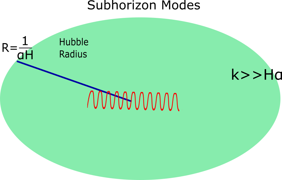
For inflationary gravitational waves, there are two cases of interest, regarding the magnitude of the mode wavelength compared to the Hubble horizon, the subhorizon and superhorizon modes. Both modes are equally important from an experimental perspective. The subhorizon modes during inflation and especially the ones with the smallest wavenumber, will be the first that will exit the horizon after inflation and during the early stages of the reheating era. These subhorizon modes (see Fig. 3), for which their wavelength is significantly smaller than the Hubble radius, that is, , or equivalently will directly be probed in about fifteen years from now, in LISA, DECIGO BBO and other large frequency gravitational waves experiments. Thus the study of these modes even analytically is of some importance. In this paper we shall mainly be interested in studying the chirality of these modes, in order to see quantitatively and at first hand their evolution. With regards to the superhorizon modes, for these their wavelength is quite larger than the Hubble radius, that is, , or equivalently (see Fig. 4).
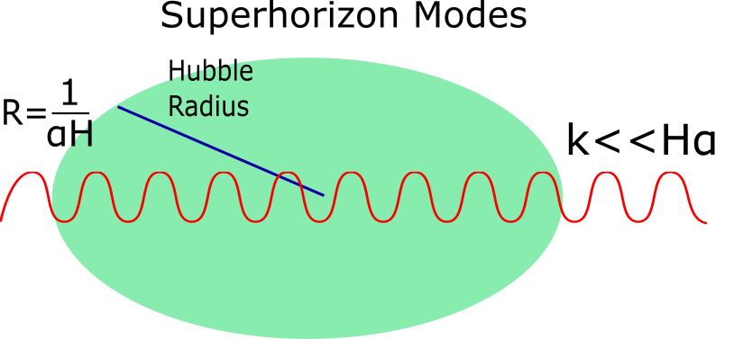
These modes will not be probed by the space interferometers, but are relevant because the CMB modes are basically modes that became superhorizon very early during the inflationary era, and were superhorizon until , where they reentered the Hubble horizon. We shall be interested in CMB superhorizon modes, so basically for modes with wavelength Mpc, or equivalently with Mpc-1. With regard to the subhorizon modes, we shall be interested for wavelengths larger than Mpc or equivalently for Mpc-1. The modes with Mpc-1 correspond to post-CMB and relevant to future primordial gravitational wave experiments, especially the modes with Mpc-1. The modes with Mpc-1 will be probed by the SKA or NANOGrav collaborations. For the above reasons, in this work we shall analytically check in a quantitative way the chirality of both subhorizon and superhorizon modes for both the axion gravity models.
Before we specify our analysis using the two axion models we discussed previously, let us consider the general behavior of the superhorizon modes in a model independent way. For the superhorizon modes, the differential equation (15) can be greatly simplified, since for these modes, their wavelengths are significantly larger compared the Hubble horizon, that is , so basically the third term in the differential equation (15) can be safely omitted, thus it reads,
| (19) |
We can find a general solution of the above differential equation, which reads,
| (20) |
thus the solution describes clearly a time-independent frozen term and an exponentially decaying mode, which is the second term in Eq. (20). We shall explicitly verify this behavior for both the canonical misalignment and kinetic axion models later on in this section.
Now our analysis will be to reveal in an analytic way the amount of chirality of the primordial gravitational waves relevant for both the CMB and future gravitational waves experiments, thus both for superhorizon and subhorizon modes, where analytical results can be obtained of course. Our strategy will be the following, since we are interested for the inflationary gravitational waves for the axion gravity models, we shall solve analytically the evolution differential equation (15), for both the left handed and right handed polarizations, considering both the superhorizon and subhorizon modes. Suppose the solutions are and , and these solutions contain two integration constants each. When analytic results can be obtained, in order to determine the integration constants, we shall assume that both solutions asymptotically in the past satisfy the Bunch-Davies initial condition, and we shall find the rest of the constants in an easy way by taking the asymptotic expansions of the solutions in two regimes, the subhorizon and superhorizon regimes, so the solutions would be , , and . Then the integrations constants can be obtained by matching the solutions for each polarization at an intermediate transition time , as follows,
| (21) | ||||
With the above initial conditions (21), the integration constants can be obtained, when both the superhorizon and subhorizon modes can be obtained. As we shall see, for the canonical misalignment axion model, this is possible, however for the kinetic axion model, analytic solutions can be obtained only for the superhorizon modes. Thus for the sake of the argument, we shall use arbitrary integration constants only for this case, just to see the behavior of the solutions as functions of the wavenumber of the modes, and also in order to reveal quantitatively the chirality between the left and right handed modes. For the analysis of the chirality between the left and right handed modes, which quantifies the difference in the propagation between left handed and right handed modes, we shall share the circular polarization function from electromagnetic studies, defined as , where an are the stokes parameters for electromagnetic waves, defined as , Alexander:2018iwy. Thus for the gravitational waves, the circular polarization function is defined as follows Satoh:2008ck,
| (22) |
for the case of subhorizon modes, while for superhorizon modes, we have,
| (23) |
Our aim in the rest of this section is to reveal the behavior of the circular polarization functions and for both the kinetic and canonical misalignment axion gravity, when this is possible.
Let us start with the canonical misalignment axion gravity. In this scenario, as we mentioned earlier, the kinetic energy and the acceleration of the axion field, namely and , are insignificant, that is , , and also note that during the inflationary era . Thus we can fix these to have significantly small values compared to the axion mass, which we shall assume that it is of the order eV for the canonical misalignment case. In view of the above considerations, by also taking into account that for the misalignment axion, we shall take and . Also for the rest of this paper, we shall assume that the Chern-Simons coupling function has the form,
| (24) |
where recall, , where is the reduced Planck mass. The values of the dimensionless free parameters and are determined by using the rule to have a viable inflationary phenomenology. We shall return to this issue later on, but now let us simplify the evolution equation (15) as much as possible in order to have a concrete quantitative idea on the behavior of the circular polarization functions and for both the subhorizon and superhorizon modes respectively. In both cases, since the modes are inflationary modes, the derivative of the gravity can be simplified as , where , and also the Ricci scalar is approximately . In addition, since the evolution is quasi-de Sitter, we assume that it is exactly a de Sitter evolution. Using these simplifications, and due to the fact that , the simplified evolution equation (15) for the left-handed polarization subhorizon modes reads,
| (25) |
while the right-handed polarization subhorizon modes satisfy,
| (26) |
The two equations can be solved analytically by simply taking into account the slowly varying form of we discussed earlier. By taking a constant value for , which we shall consider its values later on, by solving the differential equation (25) the left-handed evolution function has the following form,
| (27) | ||||
where is the confluent hypergeometric function and is the generalized Laguerre polynomial, and . Also and are integration constants that will be determined by the initial conditions (21), after we will obtain the superhorizon solutions. Accordingly, by solving the right-handed modes equation (26), we obtain the right-handed evolution function which has the following form,
| (28) | ||||
with . Also and are integration constants that in this case too will be determined by the initial conditions (21). Now let us turn our focus on superhorizon modes.
Regarding these modes, the evolution differential equation can easily be solved analytically, just in the previous case. These modes are relevant for CMB observations, and we now will measure the polarization of the superhorizon modes for small values of , in the range Mpc-1. From the beginning though, we know that superhorizon modes do freeze once they become superhorizon, so we expect a decay of the functions and after the horizon crossing, as functions of time, and in fact an exponential decay. We shall present the detailed study of the superhorizon modes here, so regarding the left-handed polarization superhorizon modes, the differential equation governing their evolution is basically the same as in Eq. (25) by simply omitting the last term, so in this case the superhorizon function which we shall denote as has the following form,
| (29) |
where and are integration constants that in this case too will be determined by the initial conditions (21). As expected, the superhorizon left-handed modes essentially freeze after the horizon crossing and they also exponentially decay as functions of the cosmic time. Also for the righthanded polarization modes, the corresponding solution reads,
| (30) |
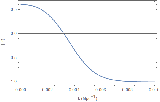
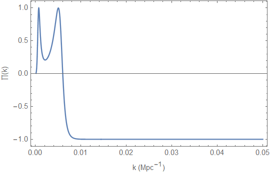
where in this case too and are integration constants that in this case too will be determined by the initial conditions (21). Also, the right-handed solution decays exponentially in time too. Now by using the initial conditions (21), and the Bunch-Davies initial condition for each mode we can find the constants of integration, which we omit for brevity. In a previous section we saw that for the model under consideration, a viable phenomenology is achieved for . This can be easily arranged for various values of the free parameters, for both the superhorizon and subhorizon modes, at the first horizon crossing though. By taking these into account, and also the values of the integration constants, and finally by considering inflationary times of the order sec, in Fig. 5 we present the behavior of the circular polarization function for modes that were subhorizon during the first stages of inflation. These subhorizon modes are directly relevant to the future gravitational waves experiments, so the wavenumber should be from Mpc-1 to Mpc-1, however we plotted the behavior from zero just to see the behavior. As it can be seen from the left plot of Fig. 5 the circular polarization function is non-zero from quite small while from , from Mpc-1 it becomes constant and equal to , however we omitted the rest of the plot, because after Mpc-1 the circular polarization function is constant. Thus the subhorizon modes ar highly polarized, since . The same applies for the superhorizon modes, and in the right plot of Fig. 5 we present the behavior of the circular polarization function for modes that were superhorizon during the first stages of inflation. As it can be seen these modes are highly polarized too, but for these modes, the wavenumber must not exceed Mpc-1, because these modes are relevant only to CMB experiments.
Now, let us turn our focus on the kinetic axion model. In this case, analytic calculations are not possible for the subhorizon case, thus even though we can obtain the superhorizon solutions, we are not able to determine the integration constants. However, just for the sake of completeness, we shall derive the analytic solutions for superhorizon modes, and by using arbitrary values for the constants of the integration, we shall demonstrate that indeed the circular polarization function is non-trivial in this case too. Recall that in the kinetic axion model, , and also . Hence it is apparent that different terms of the derivatives of the Chern-Simons coupling function dominate the evolution eventually, as we now demonstrate. Let us quote the evolution differential equations for the left and right handed polarization modes at this point, and we show how these are simplified eventually. With regard to the left-handed modes, the evolution equation of the superhorizon modes is,
| (31) |
while the right-handed modes satisfy,
| (32) |
Now regarding the term in the denominator of the second term in both the evolution equations, the term is dominant over for the values of corresponding to superhorizon modes during inflation. Also, due to the fact that for the kinetic axion we have , the term in the numerator of the second term in both the evolution equations is subdominant compared to the term , thus the evolution equations for the left-handed modes becomes,
| (33) |
while the volution equation for the right-handed modes is simplified as follows,
| (34) |
Regarding the conventions for the form of the Chern-Simons coupling function , a complete study of the Chern-Simons extended axion gravity is lacking for the kinetic axion case, we intend to do this in a future work. Thus we shall use for simplicity the conventions of the misaligned axion case, for the sake of the argument. The qualitative picture is not expected to dramatically change, when the conventions on the free parameters are changed though, and this justifies our qualitative approach here. Thus, using the conventions of the canonical misalignment axion case, for a de Sitter background evolution, the differential equations above can be solved analytically, with the left handed solution being,
| (35) |
while the right-handed solution is,
| (36) |
where , , and are arbitrary integration constants. As it can be seen, both the solutions (35) and (36) describe constant modes after horizon crossing, which both contain an exponentially decaying part. For this case, it is not possible to obtain the analytic values for these constants, because we do not know the analytic solutions for the subhorizon modes. Thus, just to see the qualitative behavior of the circular polarization function , we shall take these to be of the order of unity. We expect the overall qualitative behavior of the circular polarization function will not be affected dramatically by the actual values of the integration constants, however a formal treatment of the problem requires the exact values of the constants. Thus, using the same numerical conventions as in the canonical misalignment axion case, in Fig. 6 we plot the circular polarization function for the superhorizon modes, in the kinetic misalignment axion case.
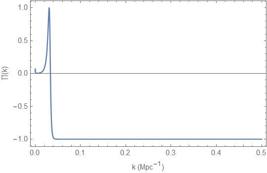
As it can be seen from Fig. 6, the circular polarization function is non-trivial in the kinetic axion model, regarding the superhorizon modes. However, the behavior obtained for the kinetic axion model is only a qualitative one, because the correct treatment requires the analytic solutions for the subhorizon modes, in order to correctly evaluate the arbitrary integration constants. However, we do not expect that the overall qualitative picture will dramatically change. The overall conclusion for both the kinetic and canonical misalignment axion models is that the tensor modes, both subhorizon and superhorizon modes are highly polarized. Thus if in future gravitational wave experiments, two signals of stochastic gravitational wave background are found, for the same frequency range, this will be a smoking gun for the presence of Chern-Simons terms in the inflationary Lagrangian. The axion models we studied in this paper are quite appealing phenomenologically, since, apart from the remnant chirality these generate, and the viable inflationary era, they also provide a refined solution for the dark matter problem. This is because the axion starts to oscillate when and for all eras for which , and its energy density redshifts as , thus it redshifts as dark matter. The difference between the two models is the time at which the oscillations begin, but beyond that difference, during the post-reheating era, the two models are basically the same. Before the reheating, the kinetic axion model might be more interesting because this model might lead to a lower reheating temperature. The physics of this model shall be studied elsewhere.
IV Conclusions
In this paper we studied the chirality of primordial gravitational waves in the context of Chern-Simons axion gravity. Specifically, the gravity was chosen to be the model, and we considered two mainstream axion field theory models, the canonical misalignment axion model and the kinetic axion model. The presence of the Chern-Simons term in the context of Einstein-Hilbert gravity ensures the chirality of the primordial gravitational waves, and this was the focus of this work, to check whether this remains true in the case of Chern-Simons gravity, with the scalar field being the axion. As we showed, since the axion and the corresponding Chern-Simons term do not significantly affect the background evolution, the model completely determines the background evolution. However, the Chern-Simons term affects the tensor perturbations explicitly, and it modifies the evolution of the two distinct polarization modes. Since we were interested in quantifying the chirality modifications caused by the Chern-Simons term we aimed to solve analytically the evolution equations of each polarization modes for each of the axion models. We considered subhorizon modes and superhorizon modes, each of which are probed or will be probed distinctly by the future gravitational wave experiments and the current and future CMB-based experiments. For the case of the misalignment axion we were able to find analytic expressions for both the superhorizon and subhorizon modes, and we were able to find all the integration constants. Accordingly, we calculated the circular polarization function for each of the subhorizon and superhorizon modes as a function of the wavenumber, and as we showed the modes are strongly chiral. In the case of the kinetic axion, the analytical study of the subhorizon modes was impossible, thus for the sake of the argument, we used the conventions of the misalignment axion case and we also showed that the spectrum is also chiral. However, the essential features of the kinetic axion gravity and its Chern-Simons extension are needed, which are lacking from the literature, and we aim to address in a future work.
Acknowledgments
This work was supported by MINECO (Spain), project PID2019-104397GB-I00 (S.D.O). This work by S.D.O was also partially supported by the program Unidad de Excelencia Maria de Maeztu CEX2020-001058-M, Spain.
References
- (1) J. Baker, J. Bellovary, P. L. Bender, E. Berti, R. Caldwell, J. Camp, J. W. Conklin, N. Cornish, C. Cutler and R. DeRosa, et al. [arXiv:1907.06482 [astro-ph.IM]].
- (2) T. L. Smith and R. Caldwell, Phys. Rev. D 100 (2019) no.10, 104055 doi:10.1103/PhysRevD.100.104055 [arXiv:1908.00546 [astro-ph.CO]].
- (3) N. Seto, S. Kawamura and T. Nakamura, Phys. Rev. Lett. 87 (2001), 221103 doi:10.1103/PhysRevLett.87.221103 [arXiv:astro-ph/0108011 [astro-ph]].
- (4) S. Kawamura, M. Ando, N. Seto, S. Sato, M. Musha, I. Kawano, J. Yokoyama, T. Tanaka, K. Ioka and T. Akutsu, et al. [arXiv:2006.13545 [gr-qc]].
- (5) S. Hild, M. Abernathy, F. Acernese, P. Amaro-Seoane, N. Andersson, K. Arun, F. Barone, B. Barr, M. Barsuglia and M. Beker, et al. Class. Quant. Grav. 28 (2011), 094013 doi:10.1088/0264-9381/28/9/094013 [arXiv:1012.0908 [gr-qc]].
- (6) J. Crowder and N. J. Cornish, Phys. Rev. D 72 (2005), 083005 doi:10.1103/PhysRevD.72.083005 [arXiv:gr-qc/0506015 [gr-qc]].
- (7) T. L. Smith and R. Caldwell, Phys. Rev. D 95 (2017) no.4, 044036 doi:10.1103/PhysRevD.95.044036 [arXiv:1609.05901 [gr-qc]].
- (8) A. Weltman, P. Bull, S. Camera, K. Kelley, H. Padmanabhan, J. Pritchard, A. Raccanelli, S. Riemer-Sørensen, L. Shao and S. Andrianomena, et al. Publ. Astron. Soc. Austral. 37 (2020), e002 doi:10.1017/pasa.2019.42 [arXiv:1810.02680 [astro-ph.CO]].
- (9) Z. Arzoumanian et al. [NANOGrav], Astrophys. J. Lett. 905 (2020) no.2, L34 doi:10.3847/2041-8213/abd401 [arXiv:2009.04496 [astro-ph.HE]].
- (10) N. S. Pol et al. [NANOGrav], [arXiv:2010.11950 [astro-ph.HE]].
- (11) M. Kamionkowski and E. D. Kovetz, Ann. Rev. Astron. Astrophys. 54 (2016) 227 doi:10.1146/annurev-astro-081915-023433 [arXiv:1510.06042 [astro-ph.CO]].
- (12) M. Denissenya and E. V. Linder, JCAP 11 (2018), 010 doi:10.1088/1475-7516/2018/11/010 [arXiv:1808.00013 [astro-ph.CO]].
- (13) M. S. Turner, M. J. White and J. E. Lidsey, Phys. Rev. D 48 (1993), 4613-4622 doi:10.1103/PhysRevD.48.4613 [arXiv:astro-ph/9306029 [astro-ph]].
- (14) L. A. Boyle and P. J. Steinhardt, Phys. Rev. D 77 (2008), 063504 doi:10.1103/PhysRevD.77.063504 [arXiv:astro-ph/0512014 [astro-ph]].
- (15) S. Kuroyanagi, T. Chiba and N. Sugiyama, Phys. Rev. D 79 (2009), 103501 doi:10.1103/PhysRevD.79.103501 [arXiv:0804.3249 [astro-ph]].
- (16) T. L. Smith, M. Kamionkowski and A. Cooray, Phys. Rev. D 73 (2006), 023504 doi:10.1103/PhysRevD.73.023504 [arXiv:astro-ph/0506422 [astro-ph]].
- (17) X. J. Liu, W. Zhao, Y. Zhang and Z. H. Zhu, Phys. Rev. D 93 (2016) no.2, 024031 doi:10.1103/PhysRevD.93.024031 [arXiv:1509.03524 [astro-ph.CO]].
- (18) W. Zhao, Y. Zhang, X. P. You and Z. H. Zhu, Phys. Rev. D 87 (2013) no.12, 124012 doi:10.1103/PhysRevD.87.124012 [arXiv:1303.6718 [astro-ph.CO]].
- (19) S. Vagnozzi, Mon. Not. Roy. Astron. Soc. 502 (2021) no.1, L11-L15 doi:10.1093/mnrasl/slaa203 [arXiv:2009.13432 [astro-ph.CO]].
- (20) Y. Watanabe and E. Komatsu, Phys. Rev. D 73 (2006), 123515 doi:10.1103/PhysRevD.73.123515 [arXiv:astro-ph/0604176 [astro-ph]].
- (21) M. Kamionkowski, A. Kosowsky and M. S. Turner, Phys. Rev. D 49 (1994), 2837-2851 doi:10.1103/PhysRevD.49.2837 [arXiv:astro-ph/9310044 [astro-ph]].
- (22) W. Giarè and F. Renzi, Phys. Rev. D 102 (2020) no.8, 083530 doi:10.1103/PhysRevD.102.083530 [arXiv:2007.04256 [astro-ph.CO]].
- (23) W. Zhao and Y. Zhang, Phys. Rev. D 74 (2006), 043503 doi:10.1103/PhysRevD.74.043503 [arXiv:astro-ph/0604458 [astro-ph]].
- (24) W. Zhao, Chin. Phys. 16 (2007), 2894-2902 doi:10.1088/1009-1963/16/10/012 [arXiv:gr-qc/0612041 [gr-qc]].
- (25) W. Cheng, T. Qian, Q. Yu, H. Zhou and R. Y. Zhou, [arXiv:2107.04242 [hep-ph]].
- (26) S. Chongchitnan and G. Efstathiou, Phys. Rev. D 73 (2006), 083511 doi:10.1103/PhysRevD.73.083511 [arXiv:astro-ph/0602594 [astro-ph]].
- (27) K. Nakayama, S. Saito, Y. Suwa and J. Yokoyama, JCAP 06 (2008), 020 doi:10.1088/1475-7516/2008/06/020 [arXiv:0804.1827 [astro-ph]].
- (28) S. Capozziello, M. De Laurentis, S. Nojiri and S. D. Odintsov, Phys. Rev. D 95 (2017) no.8, 083524 doi:10.1103/PhysRevD.95.083524 [arXiv:1702.05517 [gr-qc]].
- (29) S. Capozziello, M. De Laurentis, S. Nojiri and S. D. Odintsov, Gen. Rel. Grav. 41 (2009), 2313-2344 doi:10.1007/s10714-009-0758-1 [arXiv:0808.1335 [hep-th]].
- (30) S. Capozziello, C. Corda and M. F. De Laurentis, Phys. Lett. B 669 (2008), 255-259 doi:10.1016/j.physletb.2008.10.001 [arXiv:0812.2272 [astro-ph]].
- (31) R. G. Cai, C. Fu and W. W. Yu, [arXiv:2112.04794 [astro-ph.CO]].
- (32) R. g. Cai, S. Pi and M. Sasaki, Phys. Rev. Lett. 122 (2019) no.20, 201101 doi:10.1103/PhysRevLett.122.201101 [arXiv:1810.11000 [astro-ph.CO]].
- (33) S. D. Odintsov, V. K. Oikonomou and F. P. Fronimos, Phys. Dark Univ. 35 (2022), 100950 doi:10.1016/j.dark.2022.100950 [arXiv:2108.11231 [gr-qc]].
- (34) M. Benetti, L. L. Graef and S. Vagnozzi, Phys. Rev. D 105 (2022) no.4, 043520 doi:10.1103/PhysRevD.105.043520 [arXiv:2111.04758 [astro-ph.CO]].
- (35) J. Lin, S. Gao, Y. Gong, Y. Lu, Z. Wang and F. Zhang, [arXiv:2111.01362 [gr-qc]].
- (36) F. Zhang, J. Lin and Y. Lu, Phys. Rev. D 104 (2021) no.6, 063515 doi:10.1103/PhysRevD.104.063515 [arXiv:2106.10792 [gr-qc]].
- (37) S. D. Odintsov and V. K. Oikonomou, Phys. Lett. B 824 (2022), 136817 doi:10.1016/j.physletb.2021.136817 [arXiv:2112.02584 [gr-qc]].
- (38) M. Breitbach, J. Kopp, E. Madge, T. Opferkuch and P. Schwaller, JCAP 07 (2019), 007 doi:10.1088/1475-7516/2019/07/007 [arXiv:1811.11175 [hep-ph]].
- (39) A. D. Linde, Lect. Notes Phys. 738 (2008) 1 [arXiv:0705.0164 [hep-th]].
- (40) D. S. Gorbunov and V. A. Rubakov, “Introduction to the theory of the early universe: Cosmological perturbations and inflationary theory,” Hackensack, USA: World Scientific (2011) 489 p;
- (41) A. Linde, arXiv:1402.0526 [hep-th];
- (42) D. H. Lyth and A. Riotto, Phys. Rept. 314 (1999) 1 [hep-ph/9807278].
- (43) S. Nojiri, S. D. Odintsov and V. K. Oikonomou, Phys. Rept. 692 (2017) 1 [arXiv:1705.11098 [gr-qc]].
- (44)
S. Capozziello, M. De Laurentis,
Phys. Rept. 509, 167 (2011);
V. Faraoni and S. Capozziello, Fundam. Theor. Phys. 170 (2010). - (45) S. Nojiri, S.D. Odintsov, eConf C0602061, 06 (2006) [Int. J. Geom. Meth. Mod. Phys. 4, 115 (2007)].
- (46) S. Nojiri, S.D. Odintsov, Phys. Rept. 505, 59 (2011);
- (47) A. de la Cruz-Dombriz and D. Saez-Gomez, Entropy 14 (2012) 1717 [arXiv:1207.2663 [gr-qc]].
- (48) G. J. Olmo and D. Rubiera-Garcia, [arXiv:2203.04116 [gr-qc]].
- (49) S. Nojiri and S. D. Odintsov, Phys. Rev. D 68 (2003) 123512 doi:10.1103/PhysRevD.68.123512 [hep-th/0307288].
- (50) S. Nojiri and S. D. Odintsov, Phys. Rev. D 77 (2008) 026007 doi:10.1103/PhysRevD.77.026007 [arXiv:0710.1738 [hep-th]].
- (51) G. Cognola, E. Elizalde, S. Nojiri, S. D. Odintsov, L. Sebastiani and S. Zerbini, Phys. Rev. D 77 (2008) 046009 doi:10.1103/PhysRevD.77.046009 [arXiv:0712.4017 [hep-th]].
- (52) S. Nojiri and S. D. Odintsov, Phys. Rev. D 74 (2006) 086005 doi:10.1103/PhysRevD.74.086005 [hep-th/0608008].
- (53) S. A. Appleby and R. A. Battye, Phys. Lett. B 654 (2007) 7 doi:10.1016/j.physletb.2007.08.037 [arXiv:0705.3199 [astro-ph]].
- (54) E. Elizalde, S. Nojiri, S. D. Odintsov, L. Sebastiani and S. Zerbini, Phys. Rev. D 83 (2011) 086006 doi:10.1103/PhysRevD.83.086006 [arXiv:1012.2280 [hep-th]].
- (55) S. D. Odintsov and V. K. Oikonomou, arXiv:2001.06830 [gr-qc].
- (56) V. K. Oikonomou, Phys. Rev. D 103 (2021) no.4, 044036 doi:10.1103/PhysRevD.103.044036 [arXiv:2012.00586 [astro-ph.CO]].
- (57) V. K. Oikonomou, [arXiv:2012.01312 [gr-qc]].
- (58) S. D. Odintsov and V. K. Oikonomou, Phys. Rev. D 99 (2019) no.6, 064049 doi:10.1103/PhysRevD.99.064049 [arXiv:1901.05363 [gr-qc]].
- (59) D. J. E. Marsh, Phys. Rept. 643 (2016) 1 doi:10.1016/j.physrep.2016.06.005 [arXiv:1510.07633 [astro-ph.CO]].
- (60) M. C. D. Marsh, H. R. Russell, A. C. Fabian, B. P. McNamara, P. Nulsen and C. S. Reynolds, JCAP 1712 (2017) no.12, 036 doi:10.1088/1475-7516/2017/12/036 [arXiv:1703.07354 [hep-ph]].
- (61) P. Sikivie, Lect. Notes Phys. 741 (2008) 19 [astro-ph/0610440].
- (62) G. G. Raffelt, Lect. Notes Phys. 741 (2008) 51 [hep-ph/0611350].
- (63) A. D. Linde, Phys. Lett. B 259 (1991) 38.
- (64) A.S.Sakharov and M.Yu.Khlopov, The nonhomogeneity problem for the primordial axion field. Yadernaya Fizika (1994) V. 57, PP. 514- 516. ( Phys.Atom.Nucl. (1994) V. 57, PP. 485-487); A.S.Sakharov, D.D.Sokoloff and M.Yu.Khlopov, Large scale modulation of the distribution of coherent oscillations of a primordial axion field in the Universe. Yadernaya Fizika (1996) V. 59, PP. 1050-1055. (Phys.Atom.Nucl. (1996) V. 59, PP. 1005-1010); M .Yu.Khlopov, A.S.Sakharov and D.D.Sokoloff, The nonlinear modulation of the density distribution in standard axionic CDM and its cosmological impact. Nucl.Phys. B (Proc. Suppl.) (1999) V. 72, 105-109.
- (65) A. Aoki and J. Soda, Phys. Rev. D 96 (2017) no.2, 023534 doi:10.1103/PhysRevD.96.023534 [arXiv:1703.03589 [astro-ph.CO]].
- (66) R. T. Co, L. J. Hall and K. Harigaya, Phys. Rev. Lett. 124 (2020) no.25, 251802 doi:10.1103/PhysRevLett.124.251802 [arXiv:1910.14152 [hep-ph]].
- (67) R. T. Co, L. J. Hall, K. Harigaya, K. A. Olive and S. Verner, JCAP 08 (2020), 036 doi:10.1088/1475-7516/2020/08/036 [arXiv:2004.00629 [hep-ph]].
- (68) B. Barman, N. Bernal, N. Ramberg and L. Visinelli, [arXiv:2111.03677 [hep-ph]].
- (69) J. c. Hwang and H. Noh, Phys. Rev. D 71 (2005) 063536 doi:10.1103/PhysRevD.71.063536 [gr-qc/0412126].
- (70) A. Nishizawa and T. Kobayashi, Phys. Rev. D 98 (2018) no.12, 124018 doi:10.1103/PhysRevD.98.124018 [arXiv:1809.00815 [gr-qc]].
- (71) P. Wagle, N. Yunes, D. Garfinkle and L. Bieri, arXiv:1812.05646 [gr-qc].
- (72) K. Yagi, N. Yunes and T. Tanaka, Phys. Rev. Lett. 109 (2012) 251105 Erratum: [Phys. Rev. Lett. 116 (2016) no.16, 169902] doi:10.1103/PhysRevLett.116.169902, 10.1103/PhysRevLett.109.251105 [arXiv:1208.5102 [gr-qc]].
- (73) K. Yagi, N. Yunes and T. Tanaka, Phys. Rev. D 86 (2012) 044037 Erratum: [Phys. Rev. D 89 (2014) 049902] doi:10.1103/PhysRevD.89.049902, 10.1103/PhysRevD.86.044037 [arXiv:1206.6130 [gr-qc]].
- (74) C. Molina, P. Pani, V. Cardoso and L. Gualtieri, Phys. Rev. D 81 (2010) 124021 doi:10.1103/PhysRevD.81.124021 [arXiv:1004.4007 [gr-qc]].
- (75) F. Izaurieta, E. Rodriguez, P. Minning, P. Salgado and A. Perez, Phys. Lett. B 678 (2009) 213 doi:10.1016/j.physletb.2009.06.017 [arXiv:0905.2187 [hep-th]].
- (76) C. F. Sopuerta and N. Yunes, Phys. Rev. D 80 (2009) 064006 doi:10.1103/PhysRevD.80.064006 [arXiv:0904.4501 [gr-qc]].
- (77) K. Konno, T. Matsuyama and S. Tanda, Prog. Theor. Phys. 122 (2009) 561 doi:10.1143/PTP.122.561 [arXiv:0902.4767 [gr-qc]].
- (78) T. L. Smith, A. L. Erickcek, R. R. Caldwell and M. Kamionkowski, Phys. Rev. D 77 (2008) 024015 doi:10.1103/PhysRevD.77.024015 [arXiv:0708.0001 [astro-ph]].
- (79) H. J. Matschull, Class. Quant. Grav. 16 (1999) 2599 doi:10.1088/0264-9381/16/8/303 [gr-qc/9903040].
- (80) Z. Haghani, T. Harko and S. Shahidi, Eur. Phys. J. C 77 (2017) no.8, 514 doi:10.1140/epjc/s10052-017-5078-0 [arXiv:1704.06539 [gr-qc]].
- (81) M. Satoh, S. Kanno and J. Soda, Phys. Rev. D 77 (2008) 023526 doi:10.1103/PhysRevD.77.023526 [arXiv:0706.3585 [astro-ph]].
- (82) M. Satoh and J. Soda, JCAP 0809 (2008) 019 doi:10.1088/1475-7516/2008/09/019 [arXiv:0806.4594 [astro-ph]].
- (83) D. Yoshida and J. Soda, Int. J. Mod. Phys. D 27 (2018) no.09, 1850096 doi:10.1142/S0218271818500967 [arXiv:1708.09592 [gr-qc]].
- (84) K. Choi, J. c. Hwang and K. W. Hwang, Phys. Rev. D 61 (2000), 084026 doi:10.1103/PhysRevD.61.084026 [arXiv:hep-ph/9907244 [hep-ph]].
- (85) M. Satoh, JCAP 11 (2010), 024 doi:10.1088/1475-7516/2010/11/024 [arXiv:1008.2724 [astro-ph.CO]].
- (86) Y. F. Hang, H. J. He and C. Shen, JHEP 01 (2022), 153 doi:10.1007/JHEP01(2022)153 [arXiv:2110.05399 [hep-th]].
- (87) A. A. Starobinsky, Phys. Lett. 91B (1980) 99. doi:10.1016/0370-2693(80)90670-X
- (88) S. Alexander and E. McDonough, Phys. Lett. B 0370 (2018), 2693 doi:10.1016/j.physletb.2018.12.037 [arXiv:1811.05953 [astro-ph.CO]].