Metastable structure of photoexcited WO3 determined by the pump–probe extended X-ray absorption fine structure spectroscopy and constrained thorough search analysisJournal: Chemical Physics Letters
Abstract
We have determined the local structure of photoexcited metastable WO3 created 150 ps after 400 nm laser irradiation by the pulse pump–probe L3-edge extended X-ray absorption fine structure spectroscopy and the constrained thorough search analysis. We have found a highly distorted octahedral local structure with one of the shortest W=O bonds being further shortened to 1.66 Å while the other five bonds were elongated even though theoretical calculations predicted the reverse change. We discuss this contradiction and propose a possible structure for the metastable state.
Keywords:
Photocatalyst, Tungsten trioxide, Pump-probe EXAFS, thorough search method![[Uncaptioned image]](/html/2205.07145/assets/GraphicalAbstract.png) ††highlights: Research highlight 1
The structure of WO3 in the matastable state was determined by the pump-probe EXAFS measurement and constrained thorough search analysis
Research highlight 2
The shortest W=O bonds being further shortened to 1.66 Å Research highlight 3
The well-ordered distorted triplet cluster formation was proposed
††highlights: Research highlight 1
The structure of WO3 in the matastable state was determined by the pump-probe EXAFS measurement and constrained thorough search analysis
Research highlight 2
The shortest W=O bonds being further shortened to 1.66 Å Research highlight 3
The well-ordered distorted triplet cluster formation was proposed
1 Introduction
Semiconductor oxides are used as photocatalysts to harvest sunlight to split water into H2 and O2.[1] Electrons in the valence band, which is mainly composed of O 2 orbitals, are excited by photoirradiation to the conduction band, followed by stabilization of the photoelectrons to form the metastable state (MS), which is often assumed to be associated with surface or bulk defect sites.[1] The local structure and electronic state of the MS need to be elucidate to understand the photocatalysis of water splitting and to improve the performance of water-splitting photocatalysts.
A pump–probe (PP) X-ray absorption fine structure (XAFS) investigation of the photocatalysts using pulsed X-rays emitted from an X-ray free electron laser (XFEL) and synchrotron radiation (SR) has revealed element-specific local electronic and geometrical structures, thereby providing new scientific knowledge about photocatalysis that cannot be obtained by other techniques.[2] WO3 is used as a Z-scheme water-splitting photocatalyst that is sensitive to visible light, which is the main component of sunlight.[3] We have acquired PP X-ray absorption near edge structure (PP-XANES) spectra of WO3 after pulsed laser irradiation and have found that the MS was created within 150 ps, followed by relaxation to the ground state (GS) with a time constant of 2 ns.[4, 5, 6, 7] We proposed that the photoelectrons were trapped at distorted stoichiometric W sites in the crystal lattice, similar to the trapping of polarons, instead of at surface or bulk defects.[6] The formation time for the MS, 150 ps, was longer than that for the other oxides such as TiO2 and Fe2O3, consistent with previously-reported optical measurement results[8]. It is desirable to acquire the PP extended X-ray absorption fine structure (PP-EXAFS) spectrum to confirm the structure change because EXAFS is sensitive to local structural features such as bond lengths.[9] However, PP-EXAFS spectral measurements are much more difficult than PP-XANES measurements [6] because of the lower PP-EXAFS signal intensity. In addition compounds with a complex structure, such as WO3, require a multishell fitting which is inherently challenging. We addressed these two difficulties by taking the difference spectra between before and after photoabsorption to obtain the EXAFS spectrum of MS WO3. The difference spectra were accumulated and then analyzed using the constrained thorough search (CTS) method to elucidate the bond lengths in MS WO3.[10, 11]
In the present paper, we report the PP-EXAFS results for the structure of the MS WO3 state to clarify the local structure change and to attempt to explain the long formation time for MS WO3.
2 Experimental
2.1 Materials and methods
The WO3 was purchased from Wako Chemicals, and 50–200 nm WO3 particles were dispersed in ultrapure water. The concentration of WO3 was 2.5 mmol L-1. The WO3 jet was supplied to the cross point of the laser used for photoexcitation (Ti-sapphire with a 1 ps pulse width, 945 Hz repetition rate, and 400 nm wavelength) and the X-ray beam emitted from the Photon Factory Advanced Ring (PF-AR, 6.5 GeV, 60 mA, single bunch operation with pulse width of 100 ps, and pulse interval of 1.26 s). The fluorescence X-rays were monitored using a scintillation counter with a Cu filter to attenuate the elastic X-rays. Details of the experimental setup are available elsewhere.[4]
2.2 Analysis
The difference spectrum before and after the photoirradiation, , was accumulated, thereby reducing the possible fluctuations. The and are the spectra recorded after and before the photoirradiation, respectively. The spectrum of the MS WO3, , was obtained by assuming that was a linear combination of the spectrum of the ground state (GS), , and . , where , the fraction of MS WO3, was obtained from the XANES spectrum, as shown in Fig. S1 in the supporting information ( SI-1). was processed and analyzed using the EXAFS analysis programs REX[12] and LARCH [13], as described in SI-2. The Fourier transformation ranges of and were 5 () Å-1 and 1 () Å , respectively, so that the amount of information, , was approximately 5 ([14]. The inversely Fourier transformed data were first analyzed by a curve-fitting method using the LARCH package.[13] Further details of the structure, including bond lengths, were derived from the EXAFS spectra using the CTS method, as explained in SI-4.[10, 11, 15]
3 Results
Fig. 1 shows the EXAFS oscillation of the MS WO3, , and its Fourier transform. The main peak at 1.4 Å was inversely Fourier transformed to the -space, and the data were analyzed by one-shell curve fitting. The one-shell curve fitting results are shown in Fig. S2 and Table S1 in SI-3. We conducted the analysis using two methods. In the first method, the Debye–Waller (DW) factor was adjusted freely; in the second method, the DW factor was constrained as a function of the bond length given by Eq.S5 in SI-4. Both results indicated that the bond length contracted in the MS WO3; however, details of the structure were unclear.

We carried out the CTS analysis based on the uniform prior probability principle.[11] We assumed the followings:
- 1.
MS WO3 has uniformly distorted octahedra, similar to GS WO3.
- 2.
- 3.
EXAFS spectroscopy is sensitive to short bonds because of the
term.
The structural parameters were limited to the value of (5). The GS WO3 has a monoclinic structure in which two distorted octahedral sites are present, as shown in Table S3.[17] The bond lengths in GS WO3 have 12 different values. Two sites have a similar local structure; the corresponding W–O distances are therefore denoted as , , , , , and in Table S3 in SI-4. We intended to demonstrate that in the MS WO3, as predicted from the W L1-edge XANES results.[6] According to assumption (3) (i.e., that shorter bonds (, ) have greater contributions to the EXAFS spectra), we assumed that and were independently optimized and we constrained and , as shown in Table S3. The CTS was carried out for the four parameters , , , and with the corresponding coordination numbers, and , as shown in Table S2 and Table S3 in SI-4. Table 1 shows the CTS results that reproduced the crystal data given in Table S3 in SI-4 for the GS WO3. Note that and are approximately the same as shown in Table 1 even if the two parameters are independently changed. Fig. S5 shows the occurrence histograms. We found that the histograms for and have similar distributions and the same peak positions. Consequently, for the GS WO3, we conclude that and agreed with each other within the error.
Table 1 shows the CTS results for the MS WO3. Fig. S4 shows a comparison between the Fourier filtered and the calculated one. The observed data were well reproduced by the parameters determined by the CTS method. The R-factor(eq. S3) was 0.02. In the case of the MS WO3, we found that and were not equal and that was 0.11 Å shorter than that for the GS WO3. The histograms of and show different peak positions (Fig. 2). Bonds other than in the MS WO3 were longer than the corresponding bonds in the GS WO3, in good agreement with previously reported WO3 L1 XANES results.[6] The photoexcited MS WO3 exhibited a further distorted structure.

| sample |
| ||||||
|---|---|---|---|---|---|---|---|
| GS | 1.77 | 1.77 | 1.91 | 2.17 | 0.049 | ||
| Crystal | (1.75 | 1.77 | 1.90 | 2.13 ) | |||
| MS | 1.66 | 1.81 | 1.93 | 2.19 | 0.012 |
4 Discussion
The CTS analysis showed that the MS WO3 exhibited a further distorted structure, where the shortest W=O bond was further shortened from 1.77 Å to 1.66 Å. [6] This structure change was interpreted as follows in a previous paper.[6] The photoelectron excited by the pulsed laser would occupy the dxy orbital of W, which is on a plane perpendicular to the shortest W=O bond. The orbital is located at the bottom of the conduction band in energy scale, forming a antibonding orbital with 2 and 2 for oxygen atoms in the plane. Thus, the W–O bonds in the plane were elongated, pushing up the W atom in the direction of the shortest W=O bond.[6] As described later and in SI-7 and in SI-8, this previous interpretation is not consistent with the results of the density functional theory (DFT) and quantum mechanics/molecular mechanics (QM/MM) calculations. This discrepancy will be discussed below.
In the literature, the MS WO3 was assumed to be located in bulk or surface defect sites.[18, 19, 20] However, we disproved these possibilities because the amount of MS states is much larger than the amount of defects. Yamakata et al. recently reported that introducing defects by reducing WO3 decreased the lifetime of the MS WO3.[21] Surface defects might be less likely because the surrounding environment did not affect the lifetime of the MS WO3, as shown in SI-6. We proposed the MS WO3 should be located at the normal lattice sites in the bulk stoichiometric WO3 and be distorted from the structure of the GS WO3. Such distortion would stabilize the MS WO3, similar to the stabilization of polarons.

However, we still faced two problems. First, the DFT and QM/MM calculations for the MS WO3 local structure indicated that the less-distorted structure was stable, with the shortest W=O bond being elongated as shown in Table S5 in SI-7. Second, it was unclear why the formation of the MS WO3 structure took 150 ps. The vibration frequencies of W–O are on the order of 100 cm-1 or 3 THz or 0.3 ps. Fe2O3 hematite and CuWO4 took less than 1 ps to produce a polaronic MS.[22, 23] Thus, the simple isolated distorted MS structure should form much faster. According to the L3 edge XANES result, the W5+ was formed and was gradually changed to the MS structure.[5] Such a long time scale might be related to the collective structure change. If the single distorted structure of the MS WO3 was located in the GS WO3, it should have a greater distortion energy between the surrounding GS WO3. Thus, the theoretical calculation suggested a less distorted structure. If the two distorted MS WO3 structures gathered and were aligned along the -axis, along which the shortest W=O bonds were assumed to be headed, the distortion energy should be released. Consequently, the formation of the well-ordered distorted MS WO3 cluster shown in Fig. 3 should require a long time.
The problem with the well-ordered MS WO3 clusters is the charge balance, which should show a large negative charge. To compensate for the negative charge, holes should combine with photoexcited electrons in the well-ordered MS WO3 cluster. In this case, the recombination of photoexcited electrons and holes might be enhanced. If the spins of the hole and the photoexcited electron near the hole were parallel or in a triplet state, the well-ordered distorted MS cluster should be stabilized and had a finite lifetime; however, we had little direct evidence supporting this scenario. If we could carry out large-scale DFT calculations of the MS excited state with a large cluster size, we could support our hypothesis for the formation of such a well-defined distorted MS WO3 cluster. Such calculations will be the topic of future work.
5 Conclusions
Picosecond time-resolved W L3-edge EXAFS spectroscopy was conducted to characterize the structural change in MS WO3 in detail. We applied the CTS method to analyze the EXAFS data for the MS WO3, where one of the shortest bonds was further shortened by 0.11 Å from its original bond length, consistent with the structure proposed on the basis of W L1-edge XANES spectroscopy. This structural change in the MS WO3 led the distorted MS structure, which should be stabilized, to form well-ordered distorted clusters in conjunction with the formation of the triplet state.
6 Acknowledgement
The authors would like to express their gratitude to Prof. Masaaki Yoshida at Yamaguchi University for his technical advice and to the Japan Society for the Promotion of Science (JSPS) for their support through a Grant-in-Aid for Exploratory Research (No. 26620110), a Grant-in-Aid for Scientific Research (A) (Nos. 15H02173 and 20H00367), a Grant-in-Aid for JSPS Research Fellow (No. 15J07459), and a Grant for collaborative research in the Institute for Catalysis, Hokkaido University (No. 15A1004). The EXAFS experiments were carried out at beamline station BL-NW14A with the approval of PF-PAC (Prop. Nos. 2013G166, 2015G541, 2015G542).
See Supplemental Material at [URL will be inserted by publisher] for SI-1Estimation of the ratio of photoexcitation; SI-2 EXAFS data processing and the curve-fitting analysis; SI-3 Results of curve fitting; SI-4 Constrained thorough search; SI-5 CTS analysis of the EXAFS for the WO3 in the ground state ; SI-6 Surroundings-controlled W L3-edge XANES measurements; SI-7 Details of density functional theory (DFT) structure optimization for a single WO6 complex in monoclinic and orthorhombic environments; SI-8 Details of the QM/MM structural optimization for neutral, hole, and carrier states.
References
- [1] J. Strunk, Discover the latest research in photocatalysis combined with foundational topics in basic physical and chemical photocatalytic processes, John Wiley and Sons, 2021.
- [2] T. Yokoyama, Y. Uemura, Springer, 2017, pp. 127–132.
- [3]
R. Abe, Recent
progress on photocatalytic and photoelectrochemical water splitting under
visible light irradiation, J. Photochem. Photobiol. C 11 (4) (2010)
179–209.
doi:10.1016/j.jphotochemrev.2011.02.003.
URL https://doi.org/10.1016/j.jphotochemrev.2011.02.003 - [4]
Y. Uemura, H. Uehara, Y. Niwa, S. Nozawa, T. Sato, S. Adachi, B. Ohtani,
S. Takakusagi, K. Asakura, In situ
picosecond XAFS study of an excited state of tungsten oxide, Chem.Lett.
43 (7) (2014) 977–979.
doi:10.1246/cl.140144.
URL https://doi.org/10.1246/cl.140144 - [5]
Y. Uemura, D. Kido, Y. Wakisaka, H. Uehara, T. Ohba, Y. Niwa, S. Nozawa,
T. Sato, K. Ichiyanagi, R. Fukaya, S.-i. Adachi, T. Katayama, T. Togashi,
S. Owada, K. Ogawa, M. Yabashi, K. Hatada, S. Takakusagi, T. Yokoyama,
B. Ohtani, K. Asakura,
Dynamics
of photoelectrons and structural changes of tungsten trioxide observed by
femtosecond transient XAFS, Angew. Chem.Int.Ed 55 (2016) 1364–1367.
doi:10.1002/anie.201509252.
URL https://onlinelibrary.wiley.com/doi/full/10.1002/anie.201509252 - [6]
A. Koide, Y. Uemura, D. Kido, Y. Wakisaka, S. Takakusagi, B. Ohtani, Y. Niwa,
S. Nozawa, K. Ichiyanagi, R. Fukaya, S.-i. Adachi, T. Katayama, T. Togashi,
S. Owada, M. Yabashi, Y. Yamamoto, M. Katayama, K. Hatada, T. Yokoyama,
K. Asakura, Photoinduced
anisotropic distortion as the electron trapping site of tungsten trioxide by
ultrafast W L1-edge X-ray absorption spectroscopy with full potential
multiple scattering calculations, Phys. Chem. Chem. Phys. 20 (2020)
2615–2621.
doi:10.1039/c9cp01332f.
URL http://dx.doi.org/10.1039/C9CP01332F - [7]
Y. Uemura, T. Yokoyama, T. Katayama, S. Nozawa, K. Asakura,
Tracking the local structure
change during the photoabsorption processes of photocatalysts by the
ultrafast Pump-Probe XAFS method, Appl. Sci. 10 (21) (2020) 7818.
doi:10.3390/app10217818.
URL https://www.mdpi.com/2076-3417/10/21/7818 - [8]
I. Bedja, S. Hotchandani, P. V. Kamat,
Photoelectrochemistry of
quantized WO3 colloids: Electron storage, electrochromic, and
photoelectrochromic effects, J. Phys. Chem. 97 (42) (1993) 11064–11070.
doi:10.1021/j100144a027.
URL http://dx.doi.org/10.1021/j100144a027 - [9]
Y. Iwasawa, K. Asakura, M. Tada,
XAFS Techniques for
Catalysts, Nanomaterials, and Surfaces, Springer Nature, 2016.
doi:10.1007/978-3-319-43866-5.
URL https://doi.org/10.1007/978-3-319-43866-5 - [10] D. Kido, Y. Uemura, Y. Wakisaka, H. Ariga-Miwa, S. Takakuasgi, K. Asakura, Thorough search analysis of extended x-ray absorption fine structure data for complex molecules and nanomaterials applications, e-J.Surf.Sci.Nanotech. 18 (2020) 249–261. doi:10.1380/ejssnt.2020.249.
- [11]
D. Kido, M. M. Rahman, T. Takeguchi, K. Asakura,
Constrained thorough
search analysis of multi-edge EXAFS spectra for characterization of
bimetallic nanoparticles, Chem. Lett. 51 (5) (2022) 538–541.
doi:https://doi.org/10.1246/cl.220090.
URL https://www.journal.csj.jp/doi/10.1246/cl.220090 - [12] K. Asakura, 1st Edition, Vol. 2, World Scientific, Singapore, 1996, pp. 33–58.
- [13]
M. Newville, Larch: An
analysis package for XAFS and related spectroscopies, J.Phys.: Conf.Ser.
430 (1) (2013) 012007.
doi:10.1088/1742-6596/430/1/012007.
URL https://doi.org/10.1088/1742-6596/430/1/012007 - [14]
E. A. Stern, Number of
relevant independent points in x-ray-absorption fine-structure spectra,
Phys. Rev. B 48 (1993) 9825–9827.
doi:10.1103/PhysRevB.48.9825.
URL https://link.aps.org/doi/10.1103/PhysRevB.48.9825 - [15]
D. Kido, K. Asakura, Problems in EXAFS
analysis and its future prospects, Acc. Mater. & Surf.Res. 5 (4) (2020)
148–170.
URL https://www.hyomen.org/vol5no4 - [16]
I. Brown,
Bond
valences—a simple structural model for inorganic chemistry, Chem.Soc.Rev.
7 (3) (1978) 359–376.
doi:10.1039/CS9780700359.
URL https://pubs.rsc.org/en/content/articlelanding/1978/cs/cs9780700359 - [17]
C. J. Howard, V. Luca, K. S. Knight,
High-temperature phase
transitions in tungsten trioxide - the last word?, J.Phys., Cond.,Mat.
14 (3) (2001) 377–387.
doi:10.1088/0953-8984/14/3/308.
URL http://dx.doi.org/10.1088/0953-8984/14/3/308 - [18]
Y. Obara, H. Ito, T. Ito, N. Kurahashi, S. Thurmer, H. Tanaka, T. Katayama,
T. Togashi, S. Owada, Y. Yamamoto, S. Karashima, J. Nishitani, M. Yabashi,
T. Suzuki, K. Misawa,
Femtosecond
time-resolved x-ray absorption spectroscopy of anatase TiO2 nanoparticles
using XFEL, Struct. Dyn. 4 (4) (2017) 044033.
doi:10.1063/1.4989862.
URL https://aca.scitation.org/doi/10.1063/1.4989862 - [19]
K. Sato, K.-i. Yamanaka, S. Nozawa, H. Fukuzawa, T. Katayama, T. Morikawa,
T. Nonaka, K. Dohmae, K. Ueda, M. Yabashi, R. Asahi,
Charge
trapping process in photoexcited nitrogen-doped titanium oxides, Inorg.
Chem. 59 (15) (2020) 10439–10449.
doi:10.1021/acs.inorgchem.0c00696.
URL https://pubs.acs.org/doi/full/10.1021/acs.inorgchem.0c00696 - [20]
T. J. Penfold, J. Szlachetko, F. G. Santomauro, A. Britz, W. Gawelda, G. Doumy,
A. M. March, S. H. Southworth, J. Rittmann, R. Abela, M. Chergui, C. J.
Milne, Revealing hole
trapping in zinc oxide nanoparticles by time-resolved X-ray spectroscopy,
Nat. Commun. 9 (1) (2018) 478.
doi:10.1038/s41467-018-02870-4.
URL https://doi.org/10.1038/s41467-018-02870-4 - [21]
K. Kato, Y. Uemura, K. Asakura, A. Yamakata,
Role of oxygen vacancy in the
photocarrier dynamics of WO3 photocatalysts: The case of recombination
centers, J.Phys.Chem.C in press 126 (22) (2022) 9257–9263.
doi:10.1021/acs.jpcc.2c01662.
URL https://doi.org/10.1021/acs.jpcc.2c01662 - [22]
Y. Uemura, A. S. M. Ismail, S. H. Park, S. Kwon, M. Kim, Y. Niwa, H. Wadati,
H. Elnaggar, F. Frati, T. Haarman, N. Höppel, N. Huse, Y. Hirata, Y. Zhang,
K. Yamagami, S. Yamamoto, I. Matsuda, T. Katayama, T. Togashi, S. Owada,
M. Yabashi, U. Halisdemir, G. Koster, T. Yokoyama, B. M. Weckhuysen, F. M. F.
de Groot, Femtosecond charge
density modulations in photoexcited CuWO4, J. Phys. Chem. C 125 (13)
(2021) 7329.
doi:10.1021/acs.jpcc.0c10525.
URL https://doi.org/10.1021/acs.jpcc.0c10525 - [23]
S. Biswas, S. Wallentine, S. Bandaranayake, L. R. Baker,
Controlling
polaron formation at hematite surfaces by molecular functionalization probed
by xuv reflection-absorption spectroscopy, J.Chem.Phys. 151 (10) (2019)
104701.
doi:10.1063/1.5115163.
URL https://aip.scitation.org/doi/abs/10.1063/1.5115163 - [24]
A. V. Poiarkova, J. J. Rehr,
Multiple-scattering
x-ray-absorption fine-structure debye-waller factor calculations, Phys.Rev.B
59 (2) (1999) 948–957.
doi:10.1103/PhysRevB.59.948.
URL https://link.aps.org/doi/10.1103/PhysRevB.59.948 - [25]
M. Daniel, B. Desbat, J. Lassegues, B. Gerand, M. Figlarz,
Infrared and raman study
of WO3 tungsten trioxides and WO3, xH2O tungsten
trioxide tydrates, J. Solid State Chem. 67 (2) (1987) 235–247.
doi:10.1016/0022-4596(87)90359-8.
URL https://doi.org/10.1016/0022-4596(87)90359-8 - [26]
E. Salje, The orthorhombic
phase of wo3, Acta Cryst. B 33 (2) (1977) 574–577.
doi:10.1107/S0567740877004130.
URL https://doi.org/10.1107/S0567740877004130 - [27]
V. Blum, R. Gehrke, F. Hanke, P. Havu, V. Havu, X. Ren, K. Reuter,
M. Scheffler,
Ab
initio molecular simulations with numeric atom-centered orbitals, Comput.
Phys. Commun. 180 (11) (2009) 2175–2196.
doi:https://doi.org/10.1016/j.cpc.2009.06.022.
URL https://www.sciencedirect.com/science/article/pii/S0010465509002033 - [28]
J. D. Gale,
GULP: A
computer program for the symmetry-adapted simulation of solids, J.Chem.Soc.,
Faraday Trans. 93 (4) (1997) 629–637.
doi:10.1039/A606455H.
URL https://pubs.rsc.org/en/content/articlehtml/1997/ft/a606455h - [29]
A. A. Sokol, S. T. Bromley, S. A. French, C. R. A. Catlow, P. Sherwood,
Hybrid QM/MM embedding approach
for the treatment of localized surface states in ionic materials, Int.J.
Quantum Chem. 99 (5) (2004) 695–712.
doi:doi.org/10.1002/qua.20032.
URL https://doi.org/10.1002/qua.20032 - [30]
M. A. Sainna, S. Nanavati, C. Black, L. Smith, K. Mugford, H. Jenkins,
M. Douthwaite, N. F. Dummer, C. R. A. Catlow, G. J. Hutchings, S. H. Taylor,
A. J. Logsdail, D. J. Willock, A
combined periodic DFT and QM/MM approach to understand the radical
mechanism of the catalytic production of methanol from glycerol, Faraday
Discuss. 229 (0) (2021) 108–130.
doi:10.1039/D0FD00005A.
URL http://dx.doi.org/10.1039/D0FD00005A - [31]
M. S. Islam, S. Lazure, R.-N. Vannier, G. Nowogrocki, G. Mairesse,
Structural and computational
studies of Bi2WO6 based oxygen ion conductors, J. Mater. Chem.
8 (3) (1998) 655–660.
doi:10.1039/a707221j.
URL https://dx.doi.org/10.1039/a707221j
Supporting Information
SI-1 Estimation of the ratio of photoexcitation
SI-2 EXAFS data processing and curve fitting analysis
SI-3 Results of curve fitting
SI-4 Constrained thorough search
SI-5 CTS analysis of the EXAFS data for WO3 in the ground state
SI-6 Surroundings-controlled W L3-edge XANES measurements
SI-7 Details of the density functional theory (DFT) structure optimization for a single WO6 complex in monoclinic and orthorhombic environments
SI-8 Details about QM/MM structural optimization for neutral, hole, and carrier states
SI-1 Estimation of the ratio of photoexcitation
The photoexcitation ratio was estimated from W L3-edge XANES spectra. The valence and conduction bands for WO3 mainly consist of O 2 orbitals and W 5 orbitals, respectively. Thus, an electron is photoexcited from an O 2 to a W 5 orbital in the photoexcitation process of WO3. In W L3-edge XANES spectroscopy, an electron in a W 2 orbital is excited to a W 5 empty orbital at the edge region, which gives a strong absorption peak known as a white line. Therefore, the absorption coefficient in the white-line region decreased, as shown in Fig. S1(a). The area ratio in the XANES spectrum before and after laser irradiation was 0.95. Fig. S1(b) shows plots of the white-line area and the valence state of W for reference compounds W, WO2, and WO3. From this plot, W5+ or the MS WO3 after photoirradiation was estimated as 40 5% for the total number of W.

SI-2 EXAFS data processing and curve fitting analysis
Data processing of EXAFS was carried out using REX2000 (RIGAKU Co).[12] The EXAFS oscillation was derived from the absorption coefficient, , by subtraction of the smooth background . The is expressed as follows:
| (S1) |
where , , and are the coordination number, the bond length, and the Debye–Waller factor of the th shell, respectively, and and are the backscattering amplitude and the phase shift, respectively, for the th shell atom calculated using the FEFF8.2 code. Parameter is a wavenumber defined as
| (S2) |
where and are the mass of an electron and the Dirac constant, respectively. , , and are the incident X-ray energy, the absorption edge energy, and the correction factor for zero photoelectron kinetic energy, respectively. is the inelastic loss factor and is fixed to that for the reference compound Na2WO4. Curve fitting analysis was carried out using the LARCH package.[13] The calculated and observed data were compared using R-factor.[14]
| (S3) |
The amount of information was
| (S4) |
where is the range of the Fourier transform and is the range of the inverse Fourier transform.
SI-3 Results of curve fitting
We carried out the curve fitting analysis on the WO3 (ground state); the results are shown in Table S1. The best fitting result is shown in Fig. S2. "Constrained" or "Free" indicates that the Debye–Waller factor was treated as a function of or was optimized as a fitting parameter, as described in the main text.
| Parameter | Ground State | Photoexcited State | ||
| Constrained | Free | Constrained | Free | |
| 1.7 | 1.9 | 0.9 | 4.0 | |
| Å | 1.74 | 1.72 | 1.70 | 1.66 |
| E/eV | 4.3 | 0.1 | 4.5 | -4.1 |
| /Å2 | 0.0014∗1 | 0.016∗2 | 0.0013∗1 | 0.028∗2 |
| R-factor | 0.01 | 0.001 | 0.03 | 0.001 |
| *1 Constrained case where was determined by Eq. S5 | ||||
| *2 was optimized. | ||||

SI-4 Constrained thorough search
A constrained thorough search (CTS) analysis was carried out using a custom-made Python program[10, 15] empowered by LARCH.[13] In the CTS, we searched parameters within the -dimensional parameter space. The value of was less than the amount of information, . Thus, the constraints of several parameters were important. Because we determined the four W–O bond lengths separately, we fixed the coordination numbers for each bond as shown in Table S2. In this analysis, the and were fixed to those of the reference compound Na2WO4. The values were estimated using the equation of motion (EM) method.[24] The force constants for W–O bonds were obtained from the vibrational frequencies reported in the literature.[25] Because the force constants were strongly dependent on the bond lengths, [16] we plotted the Debye–Waller factor as a function of the W–O distance, as shown in Fig.S3. The relationship is approximated by the following equation:
| (S5) |
where is Å2 and is 2.58 Å-1. The surveyed range and steps for the CTS analysis are given in Table S2. We found all possible bond lengths in the R-factor 0.10 criterion based on the uniform prior probability principle.[11] We made histograms of the occurrence of each parameter, as shown in Fig. 2 or Fig.S5. We fitted the histogram with a Gaussian function. Each average and the distribution corresponded to the bond length and its error. Fig. S4 shows a comparison of and the calculated using the structure parameters determined by the CTS method and reported in Table S3.
| Parameter | Range / step | A | B | Temp | |
|---|---|---|---|---|---|
| Inelastic loss factor | 0.75 (Fixed) | ||||
| Correction for | |||||
| the origin of kinetic energy | /eV 17.0 (Fixed) | ||||
| Coordination number | 1 (Fixed) | ||||
| 1 (Fixed) | |||||
| 2 (Fixed) | |||||
| 2 (Fixed) | |||||
| Bond length | 1.50-1.90,0.01 step | ||||
| 1.50-1.90,0.01 step | |||||
| 1.85-2.10,0.01 step | |||||
| 2.00-2.30 ,0.01 step | |||||
| Debye–Waller factor | / Å2 | 2.58 Å-1 | 300 K |
| Site1 | Distance /Å | Site2 | Distance/ Å | Average/ Å | unified Average/ Å | CTS result / Å | ||||
| W1-O6 | 1.7434 | W2-O5 | 1.7365 | 1.74 | 1.74 | 1.770.08 | ||||
| W1-O3 | 1.7776 | W2-O4 | 1.7579 | 1.77 | 1.77 | 1.770.08 | ||||
| W1-O2 | 1.8749 | W2-O2 | 1.8899 | 1.88 | 1.90 | 1.91 0.04 | ||||
| W1-O1 | 1.9209 | W2-O1 | 1.8978 | 1.91 | (Middle) | |||||
| W1-O3 | 2.0951 | W2-O4 | 2.1009 | 2.10 | 2.14 | 2.17 0.09 | ||||
| W1-O5 | 2.1845 | W2-O6 | 2.1549 | 2.17 | (Longest) | |||||
| indicate the W–O bond length around W1, W2, and their average, respectively. | ||||||||||


SI-5 CTS analysis of the EXAFS data for WO3 in the ground state
Fig. S5 shows CTS histograms of bond lengths that satisfy the condition R-factor 0.10. Dashed lines show the fitting results obtained using a Gaussian function. The average value and standard deviation are the estimated result and its error, respectively. The structure parameters were determined and are given in Table S3; they were found to be in good agreement with those reported in the literature.[17]

SI-6 Surroundings-controlled W L3-edge XANES measurements
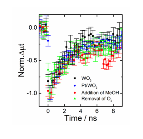
Picosecond time-resolved W L3-edge XANES measurements were carried out under controlled surroundings. The conditions were as follows: (1) Pt particles loaded onto WO3; Pt particles should enhance the charge transfer rate for excited electrons to the O2 dissolved in water. (2) Removal of oxygen by nitrogen bubbling; the decrease in O2 reduced the photoelectron consumption rate. (3) Methanol addition at a concentration of 10 vol%; the presence of methanol affected the lifetime of photo-generated holes. The concentrations of the samples differed slightly, as shown in Table S4. However, the time dependence of the change in the W L3-edge XANES spectra at 10,216 eV was the same, as shown in Fig. S6.
| Condition | Concentration of WO3 sample | Rate Constant |
|---|---|---|
| No additional treatment | 0.6 mmolL-1 | 0.5 0.1 /ns |
| Platinum loading | 0.6 mmolL-1 | 0.5 0.1 /ns |
| Addition of methanol | 2.5 mmolL-1 | 0.6 0.1 /ns |
| Removal of oxygen | 2.5 mmolL-1 | 0.5 0.1 /ns |
SI-7 Details of the density functional theory (DFT) structure optimization for a single WO6 complex in monoclinic and orthorhombic environments
This computational part of the study was based on the following working hypothesis: Photoirradiation induces local excitation around a WO6 unit. Very rapid structural relaxation occurs until the W complex is in the excited state. This structural change affects that around the W complex, and the structure transitions to the MS structure.
For the GS and MS structures, monoclinic [17] and orthorhombic WO3 structures [26] were adopted.
The computational models are shown in Fig. S7.
The central WO6 unit is surrounded by four W complexes in the same layer.
The W complexes in the upper and lower layers were omitted for simplicity.
Instead, the open valency in the O atoms were capped by H atoms. For the structure optimization, only the central WO6 unit was relaxed.
These models reproduced the original monoclinic and orthorhombic structures after the optimization process.
Electronic structure calculations were performed at the B3LYP/6-31G* level with Gaussian09.
For the excited-state calculation, time-dependent (TD) DFT was used.

Fig. S8 shows an energy diagram of the excitation and relaxation processes. Table S5 shows the results. The change in bond length in the MS state was rather symmetric; that is, shorter bonds were elongated, whereas longer ones were contracted. The distortion was decreased even compared with that of the GS. We carried out QM/MM analysis, as discussed in the next section. We could not reproduce the more distorted structure in the MS WO3, as observed in the W-L3 edge EXAFS results. This lack of reproducibility means that our working hypothesis does not match reality. In particular, our orthorhombic structure assumption for the MS state is unrealistic.
| Structural | MS(Monoclinic) | S1 state | MS(Orthorhombic) | ||
|---|---|---|---|---|---|
| parameters | Calc.( ) | Exptl. | Calc. | Calc.() | Exptl. |
| W1-O2 | 1.96(+0.07) | 1.89 | 1.93 | 1.93(+0.07) | 1.86 |
| W1-O1 | 1.97(+0.07) | 1.90 | 1.90 | 1.95(+0.09) | 1.86 |
| W1-O3 | 1.75(-0.02) | 1.77 | 1.84 | 1.93(+0.11) | 1.82 |
| W1-O6 | 1.75(0.00) | 1.75 | 1.77 | 1.89(+0.09) | 1.80 |
| W1-O3 | 2.25(+0.16) | 2.09 | 2.15 | 1.96(+0.06) | 1.90 |
| W1-O5 | 2.22(+0.07) | 2.15 | 1.97 | 1.96(-0.02) | 1.98 |
| O3-W1-O6 | 102.2(-0.4) | 102.6 | 99.0 | 92.0(-5.0) | 97.0 |
| O3-W1-O3 | 169.3(+4.6) | 164.7 | 175.7 | 178.5(-0.1) | 178.6 |
| O5-W1-O6 | 166.3(-4.6) | 170.9 | 166.7 | 176.7(+5.8) | 170.9 |

SI-8 Details about QM/MM structural optimization for neutral, hole, and carrier states
Quantum mechanical/molecular mechanical (QM/MM) modeling is a method that embeds a DFT simulation within a lattice of point charges. These point charges are to simulate the long-range dielectric and structural properties of the system and are modeled using interatomic potentials.
The QM/MM method is particularly efficient for modeling systems with localized charged sites because the model allows for structural and dielectric changes to occur around the site while still maintaining the long-range structure and properties of the bulk material. In addition, the method avoids issues with periodic defects interacting with themselves, which is an issue that periodic boundary condition (PBC) modeling encounters, particularly with charged defects.
For this study, the FHI-aims software package [27] was used as the QM calculator, and the GULP software package [28] was used for the MM calculator. These two calculators were coordinated with the ChemShell software package [29], which manages the overall QM/MM model.
QM/MM models were devised to investigate the structural changes associated with a localized electron hole, and separately a localized electron carrier within bulk WO3. These models were for the bulk material with the number of electrons within the QM-region altered to give the neutral material, as well as one missing an electron and one with an additional electron. These models were supported with neutral PBC models for the bulk material, as a basis from which to construct the QM/MM model but also to ensure accuracy and consistency, particularly for the orbital structure at the top of the valence band and at the bottom of the conduction band.
To generate the periodic model, the hybrid functional PBE0 was used, with the "light" basis sets of FHI-aims. The light basis sets were sufficient in this case because they give a sufficiently accurate representation of the geometric and electronic structure and because truly accurate values for energies were unnecessary. A -grid was needed for meV convergence.
The QM/MM model was built from the relaxed structure of the periodic model following the procedure outlined in previous work [30] and was found to be reliable for studies of other metal oxides. The chosen QM-region was a grid of W6+ ions, and all the O2 ions between them, totaling 81 atoms.
The potential energy functions used in the MM region were the Islam 1998 potentials [31]. These potentials involve Buckingham potentials between ions and a harmonic potential between anion cores and their electron shell. These simple potentials give the correct formation energies and dielectric constants for WO3 but cannot replicate the complex structure of room-temperature monoclinic I (-WO3) form. The partially covalent nature of WO3 and the different lengths for its six W–O bonds due to pseudo Jahn–Teller distortions cannot be replicated with such simple potentials. As a consequence, all the MM nuclei needed to be fixed during energy minimization to prevent instability; if allowed to relax, the active MM region would shift to a cubic structure, creating spurious interactions at each of its boundaries. In addition, any ions in the QM region bound to multiple ions in the MM region were also fixed.
Such a strict fixing of ions is necessary for the model to work but, importantly, limits what it is capable of modeling. This model can only determine structural changes within a single WO6 octahedron. If the correct structural change should be a particularly large-scale one, with multiple WO6 octahedra distorting simultaneously, a substantially larger—and potentially computationally infeasible—calculation would be required. However, any understanding gained from knowing the electronic structure at the valence and conduction band boundaries, as well as the behavior of a fully localized system, can still be insightful.
In the excited state characterized by the XAFS studies, an electron is excited from the valence band into the conduction band. This excitation should result in the formation of an electron hole and a charge carrier. To investigate how this excitation process affects the structure and bond length, the neutral structure was energy-minimized in a periodic QM/MM model and then the structure with a hole was energy-minimized using QM/MM, then again for a carrier. This approach should reveal which (if either) state would influence bond lengths.
The HOMO is nonbonding with respect to any W–O bond; however, the LUMO is bonding with respect to the W-O5 bond, and antibonding with respect to the W-O2 bond.
Bond lengths for W-O1 through W-O6 were calculated for the relaxed neutral QM/MM models. The electron–hole and charge-carrier models varied from the neutral models by containing one fewer or one more electron in the QM region, respectively. The results are shown in Table S6, and are all expressed in angstroms. Figure S9 shows the structures of the GS and MS WO3.
Reassuringly, the results for the neutral QM/MM models well match the experimental values. The maximum variance between models for any one bond length is approximately 0.04 Å.
Between the neutral and hole QM/MM models, the bond lengths do not substantially change. This result was expected because removing an electron from an orbital that is neither bonding nor antibonding with respect to any W–O bond should not strongly affect any W–O bond length. The carrier QM/MM models, by contrast, showed a lengthening of the W-O2 bond and a shortening of the W-O5 bond compared with the neutral model. This result is expected because the LUMO orbital is bonding along the W-O2 bond and antibonding along the W-O5 bond. A spin-density analysis of the carrier model showed that the additional electron is mostly located on the central W (spin +0.52), with the rest located on the nearby W (spin +0.1 to +0.2).
| QM/MM | QM/MM | QM/MM | |
|---|---|---|---|
| Neutral | Hole | Carrier | |
| W-O1 (c) | 1.78 | 1.77 | 1.78 |
| W-O2 (b) | 1.78 | 1.79 | 1.85 |
| W-O3 (a) | 1.87 | 1.87 | 1.88 |
| W-O4 (a) | 1.88 | 1.88 | 1.89 |
| W-O5 (b) | 2.09 | 2.07 | 1.99 |
| W-O6 (c) | 2.16 | 2.17 | 2.18 |

