Efficient lifting of symmetry breaking constraints for complex combinatorial problems
Abstract
Many industrial applications require finding solutions to challenging combinatorial problems. Efficient elimination of symmetric solution candidates is one of the key enablers for high-performance solving. However, existing model-based approaches for symmetry breaking are limited to problems for which a set of representative and easily-solvable instances is available, which is often not the case in practical applications. This work extends the learning framework and implementation of a model-based approach for Answer Set Programming to overcome these limitations and address challenging problems, such as the Partner Units Problem. In particular, we incorporate a new conflict analysis algorithm in the Inductive Logic Programming system ILASP, redefine the learning task, and suggest a new example generation method to scale up the approach. The experiments conducted for different kinds of Partner Units Problem instances demonstrate the applicability of our approach and the computational benefits due to the first-order constraints learned.
Under consideration for acceptance in Theory and Practice of Logic Programming (TPLP).
keywords
Answer Set Programming, Inductive Logic Programming, Symmetry Breaking Constraints1 Introduction
Finding solutions to hard combinatorial problems is important for various applications, including configuration, scheduling, or planning. Modern declarative solving approaches allow programmers to easily encode various problems and then use domain-independent solvers to find solutions for given instances. The search performance depends highly on both the encoding quality and selected solver parameters. The latter issue can partially be solved using portfolio solvers that use machine learning to select the best possible parametrization of underlying solving algorithms (Hoos et al., 2014). However, writing an optimal encoding remains a challenge that requires an experienced programmer to clearly understand the problem up to details, such as possible structures present in instances, their invariants, and symmetries.
Automatic computation of Symmetry Breaking Constraints (SBCs) can greatly simplify the programming task by extending a given encoding with constraints eliminating symmetric solution candidates, i.e., a set of candidates where each one can be obtained from another by renaming constants (Margot, 2007; Katebi et al., 2010; Walsh, 2012). Existing approaches compute SBCs either for a first-order problem encoding or for only one instance of a given problem. The latter – instance-specific methods – compute SBCs online, i.e., before or during each invocation of a solver (Puget, 2005; Cohen et al., 2006; Drescher et al., 2011). As a result, the obtained SBCs are not transferable to other instances and their computation might significantly increase the total solving time since the problem of finding SBCs is intractable. The model-based methods are usually applied offline and aim at finding general SBCs breaking symmetries of a class of instances. However, these methods are either limited to local symmetries occurring due to definitions of variable domains (Devriendt et al., 2016) or require representative sets of instances (Mears et al., 2008; Tarzariol et al., 2021) to identify SBCs that highly likely eliminate symmetries for all instances of this class. Roughly, model-based approaches apply graph-based methods, e.g., saucy (Darga et al., 2004), to find candidate symmetries of the given instances and then lift the obtained information to first-order SBCs.
The main challenge in the application of model-based approaches is that they must be able to access or generate instances that (i) comprise symmetries representative for the whole instance distribution, and (ii) are simple enough to allow the implementation to compute all of their solutions. Consider a small example of the well-studied Partner Unit Problem (PUP) (Aschinger et al., 2011; Teppan et al., 2016), which is an abstract representation of configuration problems occurring in railway safety or building security systems. As shown in Fig. 1a, the input of the problem is given by a set of units and a bipartite graph , where is a set of sensors, is a set of security/safety zones, and is a relation between and . The task is to find a partition of vertices into bags , presented in Fig. 1b, such that the following requirements hold for each bag: (i) the bag contains at most many sensors and many zones; and (ii) the bag has at most adjacent bags, where the bags and are adjacent whenever and for some . The given example shows the smallest instance representing a class of building security systems named double by Aschinger et al., 2011. Despite being the simplest instance, it has solutions, of which can be identified as symmetric (for instance, by renaming the units of a solution). Therefore, the enumeration of symmetries for PUP instances is problematic, even for the smallest and simplest ones.
(a) PUP instance
(b) A solution for the instance
The model-based method suggested by Tarzariol et al., 2021 applies an instance-specific tool for identifying symmetries of small but representative instances of a target distribution, and then generalizes respective examples by means of Inductive Logic Programming (ILP). To lift the symmetries, the method needs to investigate all solutions of the analyzed instances, making it inapplicable if no trivial satisfiable instances exist. In this work, we address such limitations and extend the framework’s applicability to combinatorial problems lacking trivial representative instances. In particular, our paper makes the following contributions:
- •
We propose a new definition of the ILP learning task and a corresponding implementation for the input generation, which allow the approach to scale with respect to the number of answer sets of the analyzed instances, thus, learning efficient first-order constraints.
- •
We provide a novel conflict analysis method for the learning system ilasp (Law et al., 2020) that significantly improves the efficiency of the constraint learning.
- •
We present an extensive experimental study conducted on three kinds of PUP benchmarks shows that the new method clearly outperforms the legacy approach in terms of learning and solving performance.
2 Background
In this section, we briefly introduce basic notions of Answer Set Programming, Inductive Logic Programming, and the work by Tarzariol et al., 2021, which uses ILP to learn first-order constraints from symmetries of ground ASP programs.
2.1 Answer Set Programming
Answer Set Programming (ASP) is a declarative programming paradigm based on non-monotonic reasoning and the stable model semantics (Gelfond and Lifschitz, 1991). Over the past decades, ASP has attracted considerable interest thanks to its elegant syntax, expressiveness, and efficient system implementations, successfully adopted in numerous domains like, e.g., configuration, robotics, or biomedical applications (Erdem et al., 2016; Falkner et al., 2018). We briefly present the syntax and semantics of ASP, and refer the reader to textbooks (Gebser et al., 2012; Lifschitz, 2019) for more in-depth introductions.
Syntax.
An ASP program is a set of rules of the form:
where stands for default negation and , for , are atoms. An atom is an expression of the form , where is a predicate, is a possibly empty vector of terms, and the predicate (with an empty vector of terms) represents the constant false. Each term in is either a variable or a constant. A literal is an atom (positive) or its negation (negative). The atom is the head of a rule , denoted by , and the body of includes the positive or negative, respectively, body atoms and . A rule is called a fact if , and a constraint if .
Semantics.
The semantics of an ASP program is given in terms of its ground instantiation , which is obtained by replacing each rule with its instances obtained by substituting the variables in by constants occurring in . Then, an interpretation is a set of (true) ground atoms occurring in that does not contain . An interpretation satisfies a rule if and imply , and is a model of if it satisfies all rules . A model of is stable if it is a subset-minimal model of the reduct , and we denote the set of all stable models, also called answer sets, of by .
2.2 Inductive Logic Programming
Inductive Logic Programming (ILP) is a form of machine learning whose goal is to learn a logic program that explains a set of observations in the context of some pre-existing knowledge (Cropper et al., 2020). Since its foundation, the majority of research in the field has addressed Prolog semantics although applications in other paradigms appeared in the last years. The most expressive ILP system for ASP is Inductive Learning of Answer Set Programs (ilasp), which can solve a variety of ILP tasks (Law et al., 2014; Law et al., 2021).
Learning from Answer Sets.
A learning task for ilasp is given by a triple , where an ASP program defines the background knowledge, the set comprises two disjoint subsets and of positive and negative examples, and the hypothesis space is defined by a language bias , which limits the potentially learnable rules (Law et al., 2014). Each example is a pair called Context Dependent Partial Interpretation (CDPI), where (i) is a Partial Interpretation (PI) defined as pair of sets of atoms , called inclusions () and exclusions (), respectively, and (ii) is an ASP program defining the context of PI . Given a (total) interpretation of a program and a PI , we say that extends if and . Given an ASP program , an interpretation , and a CDPI , we say that is an accepting answer set of with respect to if such that extends .
Each hypothesis learned by ilasp must respect the following criteria: (i) for each positive example , there is some accepting answer set of with respect to ; and (ii) for any negative example , there is no accepting answer set of with respect to . If multiple hypotheses satisfy the conditions, the system returns one of those with the lowest cost. By default, the cost of each rule corresponds to its number of literals (Law et al., 2014); however, the user can define a custom scoring function for defining the rule costs. Law et al., 2018 extend the expressiveness of ilasp by allowing noisy examples. With this setting, if an example is not covered, i.e., there is an accepting answer set for if it is negative, or none if is positive, the corresponding weight is counted as a penalty. If no dedicated weight is specified, the example’s weight is infinite, thus forcing the system to cover the example. Therefore, the learning task becomes an optimization problem with two goals: minimize the cost of and minimize the total penalties for the uncovered examples.
The language bias for the ilasp learning task is specified using mode declarations. Constraint learning, i.e., when the search space exclusively consists of rules with , requires only mode declarations for the body of a rule: #modebR,P,E. In this definition, the optional element R is a positive integer, called recall, which sets the upper bound on the number of mode declaration applications in each rule. P is a ground atom whose arguments are placeholders of type var(t) for some constant term t. In the learned rules, the placeholders will be replaced by variables of type t. For each rule, there are at most variables and literals in the body, which are both equal to by default. Finally, E is an optional modifier that restricts the hypothesis space further, limited in our paper to the anti_reflexive and symmetric options that both work with predicates of arity . When using the former, the atoms of the predicate P should be generated with two distinguished argument values, while rules generated with the latter take into account that the predicate P is symmetric.
In a constraint learning task, just as in other ILP applications (Cropper and Dumančić, 2020), the language bias must be defined manually for each ASP program . A careful selection of the bias is essential since a too weak bias might not provide enough limitations for a learner to converge. In contrast, a too strong bias may exclude solutions from the search space, thus resulting in sub-optimal learned constraints.
Conflict Driven Inductive Logic Programming (CDILP).
Several ilasp releases have been developed in the last years, extending its learning expressiveness and applying more efficient search techniques (Law et al., 2020). Recently, Law, 2022 introduced CDILP – a new search approach that overcomes the limitation of previous ilasp versions regarding scalability with respect to the number of examples and further aims at efficiently addressing tasks with noisy examples. The approach exploits a set of coverage constraints, each defined by a pair , where is a CDPI and is a propositional formula over identifiers for the rules in . The formula is defined such that, for any , if does not respect , then does not cover . CDILP interleaves the search for an optimal hypothesis (for the current ) with a “conflict analysis” phase. In this phase, ilasp identifies (at least) one example not covered by , which was not determined by the current ; then, it creates a new conflict for and adds it to . If such an example does not exist, ilasp returns the current as an optimal solution. Otherwise, the system repeats the procedure with the updated set of conflicts. Using the Python interface, PyLASP, one can apply different conflict analysis methods as long as they are proven to be valid, i.e., a method must terminate and compute formulas such that the current hypothesis does not respect them. This requirement guarantees that the CDILP procedure terminates and returns an optimal hypothesis for the learning task.
There are currently three built-in methods for conflict analysis in ilasp, denoted by , , and , each of which determines a coverage constraint for an example that is not covered by a given hypothesis . In the most stringent case, , ilasp computes a coverage constraint that is satisfied by exactly those hypotheses that cover . Identifying such a comprehensive coverage formula has the advantage that any example will be analyzed in at most one iteration, so that ilasp with for conflict analysis usually requires a small number of iterations only. On the other hand, computing such a precise coverage formula is complex, meaning that an iteration can take long time. For this reason, and were introduced. Both methods yield smaller formulas that can be computed in less time. While this can lead to more iterations of CDILP, in some domains, the overall runtime benefits from significantly shorter iterations. However, our preliminary investigations showed that, for highly combinatorial PUP instances, even and struggle to compute coverage constraints in acceptable time. In this work, we thus introduce a new conflict analysis method that brings significant improvements over , , and on PUP instances.
2.3 Lifting SBCs for ASP
Tarzariol et al., 2021 presented an approach to lift ground SBCs for ASP programs using ILP. Their system takes four kinds of inputs: (i) an ASP program modeling a combinatorial problem; (ii) two sets and of small satisfiable instances representative for a practical problem solved using ; (iii) the hypothesis space ; and (iv) the Active Background Knowledge as an ASP program comprising auxiliary predicate definitions and constraints learned so far. The generalization set contains instances used to generate positive examples that the set of learned constraints must preserve. As a result, we increase the likelihood for the learned constraints to generalize beyond the training examples. The instances of the training set are passed to the instance-specific symmetry breaking system sbass (Drescher et al., 2011) to identify the symmetries of each instance in . The output of sbass, , is a set of permutation group generators (also called permutations) subsuming groups of symmetric answer sets for the analyzed ground program. The framework by Tarzariol et al., 2021 uses this information to define the positive and negative examples for an ILP task and applies ilasp to solve it. The negative examples are associated with a weight, as the system aims at constraints that remove as many symmetric answer sets as possible but does not require eliminating all of them.
In their subsequent work, Tarzariol et al., 2022b discuss four approaches for creating training examples with sbass for ground programs , obtained by grounding with the instances . In particular, enum enumerates all answer sets of and classifies each solution as a positive or negative example, according to the common lex-leader approach. That is, if an answer set can be mapped to a lexicographically smaller, symmetric answer set using the permutations , i.e., if is dominated, it will produce a negative example. Otherwise, yields a positive example. In both cases, the inclusions are , where denotes the set of atoms occurring in , the exclusions are , and the context is . On the other hand, the fullSBCs approach exploits the clingo API to interleave the solving phase, which returns a candidate answer set , with the analysis of all its symmetric solutions. Thanks to the properties of permutation groups (Sakallah, 2009), fullSBCs can determine all symmetric answer sets by repeatedly applying the permutations to until no new solutions can be obtained. This approach leads to a partition of the answer sets for an instance, where every partition cell consists of symmetric solutions. For each obtained cell, the system labels the smallest answer set as a positive example and all remaining ones as negative examples, thus achieving full rather than partial symmetry breaking, while the enum approach yields the latter only.
Tarzariol et al., 2022b evaluate the performance of their methods on three versions of the pigeon-hole problem and the house-configuration problem (Friedrich et al., 2011). The they use contains predicates emulating arithmetic built-ins, and the search space is split to apply the learning framework iteratively and thus increase the learning efficiency. Given that the considered problem instances are defined in terms of unary predicates and those in the training set have a small number of solutions (from about a dozen up to a few hundred), the suggested formulation of the ILP task admits a fast learning of first-order constraints speeding up the solving of (unsatisfiable) instances. However, instances of complex application problems lack the presupposed characteristics, rendering the previously proposed approaches inapplicable and calling for a more scalable handling of training instances.
3 Method
This section presents an alternative version of the framework introduced by Tarzariol et al., 2021, extending its applicability. First, we propose a revised ILP learning task and procedures necessary to define inputs of this task for difficult combinatorial problems, as illustrated in Fig. 2. Then, we describe a new conflict analysis method for the ilasp system enabling efficient constraint learning to handle this revised task.
3.1 Revised ILP Task
Training Examples.
Tarzariol et al., 2021 propose approaches to the example generation for an ILP learning task, which yield a number of examples proportional to the number of solutions for each problem instance in . However, for difficult problems with many symmetries, even the simplest instances might yield a large number of answer sets. Their enumeration might thus take unacceptably long time. Moreover, even if the enumeration succeeds, the number of obtained examples is often too large to be handled by ilasp. To overcome these issues, we propose two scalable approaches to the generation of examples for each instance in based on the enum and fullSBCs strategies by Tarzariol et al., 2021. The scalable enum strategy generates examples from a portion of solutions, which are sampled from at most random answer sets. For each candidate solution, the lex-leader criterion is applied to determine whether another symmetric answer set dominates it. This approach does not guarantee a fixed ratio between positive and negative examples, and it might fail to identify symmetric answer sets, as inspecting single applications of permutation group generators does not achieve full symmetry breaking (Sakallah, 2009). Nevertheless, the fixed number of considered answer sets provides means to limit the time required for the definition of a learning task. The scalable fullSBCs approach creates a set of examples configured by two parameters: (i) cellsdefines the number of cells of symmetric solutions to analyze; and (ii) max_cell_sizelimits the maximal number of negative examples generated per cell. For each cell, the approach adds the first max_cell_size symmetric answer sets as negative examples. Next, it explores the whole cell of symmetric solutions and takes the smallest one as a positive example. As a result, this method generates a controlled number of positive and negative examples, regardless of how many solutions there may be for a given instance. In fact, at most cells many positive and many negative examples can be obtained in total.
Background Knowledge.
Learning SBCs that improve the grounding and solving efficiency is crucial for difficult combinatorial problems. Therefore, the background knowledge should provide necessary auxiliary predicates that allow an ILP system to incorporate such constraints in the search space. Previous formulations of for learning SBCs have issues with expressing appropriate constraints since the provided predicates do not take the structure of problem instances into account. In this paper, we propose a new version of comprising two new types of auxiliary predicates. The first type encodes local properties of nodes in an input graph, while the second enables a more efficient constraint representation. That is, for two different nodes N and M, the predicate close(N,M) holds if these nodes share a common neighbor. In case of bipartite graphs containing two types of nodes, A and B (standing for sensors and zones in case of PUP instances), we define two versions of this auxiliary predicate, distinguishing the two types by closeA/2 and closeB/2. The second auxiliary predicate introduces an ordering on value assignments as follows: let and be the domains of two variables X and Y, and p(X,Y) be a binary predicate that holds for at most one value per in each answer set. Then, we define the following auxiliary predicate:
If pGEQ(X,Y) is true, we know that p(X’,Y) holds for some value X’ equal to X or greater. A constraint may then contain pGEQ(Y,Y) instead of the equivalent test p(X,Y), Y <= X, thus reducing the ground instantiation size. Moreover, this encoding can bring benefits for solving as well, as we obtain a more powerful propagation (Crawford and Baker, 1994).
From a technical perspective, the framework presented by Tarzariol et al., 2021 runs sbass on a ground program resulting from the union of , an instance , and . The inclusion of caused no difference in the symmetries for their approach (without iterative constraint learning), given that the introduced auxiliary predicates do not affect atoms occurring in . On the other hand, the predicate pGEQ/2 alters the identification of symmetries for atoms over the predicate p/2 contained in . Hence, we do not necessitate to contribute to a ground program passed to sbass, as indicated in Fig. 2.
Language Bias.
To address difficult combinatorial problems, we suggest the following set of mode declarations to define the search space :
Assuming that the predicate r/2 specifies the graph provided by an instance, the mode declaration in the first line expresses that one such atom can occur per constraint. Then, for each close/2 or pGEQ/2 predicate in , we include a respective mode declaration as in the second and third lines. Moreover, if atoms over another predicate q/2 occur in , but not in , we supply a mode declaration of the last kind, where considering binary predicates is sufficient for PUP instances. Let us notice that only one type t of variables is used for all mode declarations. In this way, there is no restriction on the variable replacements, and we may explore inherent yet hidden properties of the input labels. Furthermore, we introduce an alternative scoring function assigning the cost to each rule . For every literal obtainable from the mode declarations, we overwrite its default cost with a custom cost, except for literals over domain predicates like, e.g., r/2. For literals over other predicates, in case the same variable is used for both of the contained arguments, the cost is , and otherwise. For example, the cost of the constraint :- pGEQ(V1,V1), close(V1,V2), q(V2,V3). would be equal to with the default scoring function but with our custom costs.
3.2 Conflict Analysis
As discussed in Section 2.2, ilasp’s Conflict Driven ILP (CDILP) approach requires a conflict analysis method that, given a hypothesis and an example that does not cover, returns a coverage formula . For ilasp to function correctly, this formula must (i) not be satisfied by , and (ii) be satisfied by every hypothesis covering .
Ilasp has several built-in methods for conflict analysis, some of which are described by Law, 2022. However, for learning tasks with hypothesis spaces that consist of constraints only, these methods all behave equivalently when processing positive examples. For positive examples such that has many answer sets, the built-in methods can return extremely long coverage formulas that also take long time to compute. For this reason, we define a new conflict analysis method leading to shorter coverage constraints that can be computed much faster.
Definition 1
Let be a learning task such that consists of constraints, and let be a positive example. For any that does not cover , the subsumption-based conflict analysis method returns the formula , where denotes that subsumes .
Example 1
Consider a scenario such that ilasp is run on a task with the language bias given in the previous subsection. At some point in the execution, may generate the hypothesis . Within the hypothesis space computed by ilasp,11 1 This space is smaller than the full hypothesis space as isomorphic rules are discarded. For instance, :- q(V2, V2). is isomorphic to :- q(V1, V1). and thus not considered by ILASP. the first rule is only subsumed by itself, and the second rule is subsumed by the following rules:
:- q(V1,V1).                      :- not pGEQ(V1,V1), q(V1,V1).
:- q(V1,V2).                      :- not pGEQ(V1,V1), not pGEQ(V1,V2), q(V1,V2).
:- pGEQ(V1,V1).                   :- not pGEQ(V1,V1), not pGEQ(V2,V1), q(V1,V2).
:- pGEQ(V1,V2).                   :- not pGEQ(V1,V1), not pGEQ(V2,V2), q(V1,V2).
:- not pGEQ(V1,V1), q(V1,V2).     :- not pGEQ(V1,V2), not pGEQ(V2,V1), q(V1,V2).
:- not pGEQ(V1,V2), q(V1,V2).     :- not pGEQ(V1,V2), not pGEQ(V2,V2), q(V1,V2).
:- not pGEQ(V2,V1), q(V1,V2).     :- not pGEQ(V2,V1), not pGEQ(V2,V2), q(V1,V2).
:- not pGEQ(V2,V2), q(V1,V2).
Let be the first rule in and be the rules that subsume the second rule. In this case, for any positive example that is not covered by , we obtain the coverage constraint .
The following theorem shows that is a valid method for conflict analysis for positive examples, provided that the hypothesis space contains constraints only. This means that in our application domain, when using the method for some or all of the positive examples, ilasp is guaranteed to return an optimal solution for any learning task.
Theorem 1
Let be a learning task such that consists of constraints, and let be a positive example. For any that does not cover :
- 1.
does not satisfy .
- 2.
Every that covers satisfies .
Proof 3.2.
- 1.
For each , implies that is not satisfied by . Thus, cannot satisfy any of the disjuncts of , i.e., it does not satisfy .
- 2.
Assume for contradiction that some covers but does not satisfy . Then, by the definition of covering , there is some answer set that extends . As does not satisfy , must include constraints that subsume each of the constraints in . This means that . Hence, contradicts the condition that does not cover .
The advantage of the method for conflict analysis, over the methods that are already built-in to ilasp, is that this method does not need to compute answer sets of (for an uncovered example with context ). In other words, it does not need to consider the semantics of the current hypothesis and can instead focus on purely syntactic properties. In combinatorial problem domains, where finding answer sets can be computationally intensive, our preliminary experiments showed that is much faster than the existing conflict analysis methods of ilasp. On the other hand, the syntactic coverage constraints generated by tend to be more specific than the semantic constraints computed by ilasp’s built-in methods. That is, the formulas determined by apply to fewer hypotheses and cut out fewer solution candidates, which in turn means that more (yet considerably faster) iterations of the CDILP procedure are required.
The method is closely related to the ILP system Popper (Cropper and Morel, 2021), which also identifies syntactically determined constraints based on subsumption. Specifically, when Popper encounters a hypothesis entailing an atom that should not be entailed (a negative example for Popper), all hypotheses subsuming are discarded (as these would also entail the atom). Just like , since Popper uses syntactically determined constraints, it can compute these very quickly but may need many more iterations (compared to the semantic conflict analysis methods of Ilasp). While both approaches are closely linked, Popper learns under Prolog semantics. Therefore, Popper cannot reason about logic programs with multiple answer sets and is inapplicable for learning ASP constraints in the combinatorial problem domains we address.
PyLASP Script.
The method is essential to compute coverage formulas for positive examples obtained from the generalization set , including instances with a large number of answer sets, in acceptable time. However, for other examples, the existing conflict analysis methods of ilasp are better suited, as the obtained formulas are more informative. Hence, we extended the default PyLASP script of ilasp with means to specify examples requiring usage by dedicated identifiers, associated with instances in on which clingo takes more than seconds for enumerating the answer sets.
4 Experiments
For testing our new method, we decided to use PUP configuration benchmarks (Teppan et al., 2016). We applied our framework to PUP instances supplied by Aschinger et al., 2011, studying the double, doublev, and triple instance collections with . Instances of the same type represent buildings of similar topology with scaling parameters that follow a common distribution. Although the benchmark instances are synthetic, they represent a relevant configuration problem concerning safety and security issues in public buildings, like administration offices or museums. In addition, the scalable synthetic benchmarks are easy to generate and analyze. That is, the nodes corresponding to rooms are labeled in a specific order, and the topologies follow a clear pattern. The PUP instances and further details are provided by Tarzariol et al., 2022a.
In all three experiments, we learn first-order constraints using the same inputs to the ILP task, except for the two instance sets and : for , we pick the smallest representative instance of the selected type, while comprises the three smallest satisfiable instances other than the one in . Components of the ILP task shared between the experiments with different kinds of instances include: (i) the input program as an ASP encoding of PUP that comprises no SBCs and originates from work by Dodaro et al., 2016, where it is referred to as ENC1; (ii) the background knowledge defining the auxiliary predicates closesensors/2, closezones/2, unit2zoneGEQ/2, and unit2sensorGEQ/2; and (iii) the language bias with mode declarations for the auxiliary predicates in as well as the predicates zone2sensor/2 and partnerunits/2, the latter taking the roles of r/2 and q/2 according to the scheme described in Section 3.1.
For each PUP instance type, we tested the two proposed approaches (scalable enum and scalable fullSBCs) combined with two versions of the scoring function: the default function of ilasp as well as the custom costs introduced in Section 3.1. With both example generation approaches, the sampling of answer sets was done using the --seed <> option of clingo (v5.4.0). We executed the experiments using different random seeds to counterbalance the impact of randomness and get more reliable estimates of the relative learning and solving performance. For comparing the two approaches, we sampled the same number of examples configured by for scalable enum and for scalable fullSBCs. We limited the learning time to one hour, interrupting the process in case no positive or negative examples could be obtained from the analysis by sbass.
In preliminary investigations, we tried the default PyLASP script of ilasp (v4.1.2) as well as the one we devised to apply the method for conflict analysis to positive examples from . As expected, no run with the default script could be finished within one hour, and we thus focus below on results obtained with our new PyLASP script.
The learning efficiency for all three PUP instance types is such that scalable fullSBCs yields more successful ILP tasks, i.e., tasks solved by ilasp within the time limit, than scalable enum.22 2 The results reflect the learning setting leading to the fastest runtime, using the alternative ordering ord but no sat mode (Tarzariol et al., 2022b). Detailed records are provided by Tarzariol et al., 2022a. Using the scalable fullSBCs strategy and different random seeds, we were able to finish ilasp runs with seeds for double, for doublev, and for triple. The application of scalable enum resulted in only , , or successful runs, respectively, with some of the seeds. Note that several scalable enum runs had to be canceled because the generated ILP tasks were partial, i.e., without either positive or negative examples, so that trivial optimal hypotheses make learning with ilasp obsolete. As scalable fullSBCs is the by far more successful example generation strategy, we restrict the following considerations of solving performance to constraints learned with it.
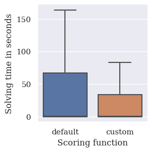
(a) Results for PUP double
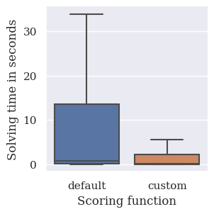
(b) Results for PUP doublev
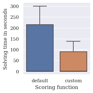
(c) Results for PUP triple
Next, we compare the solving performance of clingo relative to constraints learned with the default scoring function of ilasp or the custom costs distinguishing domain predicates and variable recurrences as described in Section 3.1. To this end, we consider those of the random seeds for which ilasp runs finished successfully with both of the scoring functions, and then provide the learned constraints as background knowledge to clingo along with a PUP instance. Each clingo run is limited to seconds solving time, and Fig. 3 displays box plots as well as average runtimes (Avg), standard deviation (Std), and number of timeouts with the total number of runs in parentheses (TO) for the double, doublev, and triple instances. For all three PUP instance types and especially the hard instances whose runtime is above average, we observe significant speed-ups due to constraints learned by means of the custom scoring function. In fact, the custom costs give preference to first-order constraints whose ground instances apply and prune the search space more directly, thus benefiting the solving performance of clingo. We also applied the Wilcoxon Signed-Rank test (Wilcoxon, 1992) for non-normally distributed runtimes, which confirms that the observed differences are statistically significant.
Finally, we contrast the best-performing learning setting, i.e., the scalable fullSBCs strategy for example generation along with our custom scoring function for assigning costs to constraints, with originally proposed ASP encodings of PUP and instance-specific symmetry breaking. In detail, Tables 2–3 show runtime results for the following systems and encodings: (i) clingoon the plain ENC1 encoding; (ii) clingoon ENC1 augmented with the most efficient learned constraints among those aggregated in Fig. 3 as ; (iii) clingoon the advanced ENC2 encoding (Dodaro et al., 2016), incorporating hand-crafted static symmetry breaking as well as an ordered representation (Crawford and Baker, 1994) of assigned units similar to pGEQ/2 in Section 3.1; (iv) sbassfor permutation and ground SBCs computation on ENC1; and (v) claspπdenoting the solving time of clingo on ENC1 augmented with ground SBCs by sbass.33 3 In the online usage of instance-specific symmetry breaking, the runtimes of sbass and claspπ add up. PUP instances are named according to the scheme [un-]type-zones, where un indicates unsatisfiability due to including one unit less than required, type denotes the double, doublev, and triple collections by dbl, dblv, or tri, and the number of zones provides a measure of size. Each run is limited to seconds, and the TO entries mark unfinished runs.
Regarding different PUP encodings, ENC2 leads to more robust clingo performance than the simpler ENC1 encoding, even if ground SBCs from sbass are included for claspπ. That is, apart from a few shorter runs with ENC1 on satisfiable instances (dbl-30, dblv-45, tri-18, and tri-21) in Tables 2–3, clingo scales better with ENC2, never times out on instances finished with ENC1 or possibly claspπ, and is able to solve some instances (dbl-50, un-tri-12, and un-tri-15) on which the latter two settings fail. Considering that sbass produces ground SBCs within the time limit for all instances, the better performance with ENC2 suggests that its hand-crafted static symmetry breaking approach provides a more economic trade-off between the compactness and completeness of introduced SBCs. However, we checked that static symmetry breaking by unit labels counteracts sbass to detect any instance-specific symmetries, so that ENC2 commits to value symmetries only.
file=PUP_double.csv, head to column names, before reading=, tabular=lrrrrr, table head=
ENC1 ABK ENC2 SBASS
, command=\Instance \BASE \ABK \ENC \SBASS \CLASP, table foot=
file=PUP_doublev.csv, head to column names, before reading=, tabular=lrrrrr, table head=
ENC1 ABK ENC2 SBASS
, command=\Instance \BASE \ABK \ENC \SBASS \CLASP, table foot=
file=PUP_triple.csv, head to column names, before reading=, tabular=lrrrrr, table head=
ENC1 ABK ENC2 SBASS
, command=\Instance \BASE \ABK \ENC \SBASS \CLASP, table foot=
Indeed, when comparing ENC2 to clingo on ENC1 with first-order constraints learned by ilasp as , we observe further significant performance improvements thanks to our approach, particularly on the unsatisfiable instances in Tables 2–3. That is, the learned enables clingo to solve the considered PUP instances of three different types and efficiently prunes the search space, which must be fully explored in case of unsatisfiability. We checked that the learned constraints exploit the topology of instances to restrict the assignable units, particularly using the predicate unit2sensorGEQ/2 for referring to the assignment of sensors. The specific sets of efficient first-order constraints learned for each of the three PUP instance types are provided in our repository (Tarzariol et al., 2022a).
5 Conclusions
This paper introduces an approach to learn first-order constraints for complex combinatorial problems, which cannot be successfully tackled by previous, less scalable methods (Tarzariol et al., 2022b). We devised and implemented two configurable strategies to generate the examples for an ILP task, and extended the background knowledge by auxiliary predicates admitting a more compact representation and potentially stronger propagation of constraints on value assignments. Moreover, we introduced a custom scoring function taking the ground instances of first-order constraints into account, along with a new conflict analysis method for ilasp that enables a much faster handling of positive examples with many answer sets. The revised learning framework taking all proposed techniques together is able to learn efficient first-order constraints from non-trivial problem instances, as demonstrated on three kinds of PUP benchmarks – a challenging configuration problem. In the future, we hope to introduce automatic (re-)labeling schemes for constants appearing in instances to exploit common problem structure in a less input-specific way. Moreover, we aim at extending our learning framework further to enable the model-based analysis and breaking of symmetries for practically important optimization problems. Beyond graph-oriented applications, we plan to expand the scope of our constraint learning methods to further areas, such as scheduling domains with symmetries among tasks and resources, e.g., several instances of products, machines, or workers with the same skills.
Acknowledgments.
This work was partially funded by KWF project 28472, cms electronics GmbH, FunderMax GmbH, Hirsch Armbänder GmbH, incubed IT GmbH, Infineon Technologies Austria AG, Isovolta AG, Kostwein Holding GmbH, and Privatstiftung Kärntner Sparkasse. We thank the anonymous reviewers for their valuable suggestions and comments.
References
- Aschinger et al., (2011) Aschinger, M., Drescher, C., Friedrich, G., Gottlob, G., Jeavons, P., Ryabokon, A., and Thorstensen, E. Optimization methods for the partner units problem. In International Conference on Integration of Artificial Intelligence and Operations Research Techniques in Constraint Programming 2011, volume 6697 of Lecture Notes in Computer Science, pp. 4–19. Springer.
- Cohen et al., (2006) Cohen, D., Jeavons, P., Jefferson, C., Petrie, K., and Smith, B. 2006. Symmetry definitions for constraint satisfaction problems. Constraints, 11, 2-3, 115–137.
- Crawford and Baker, (1994) Crawford, J. and Baker, A. Experimental results on the application of satisfiability algorithms to scheduling problems. In AAAI Conference on Artificial Intelligence 1994, pp. 1092–1097. AAAI Press.
- Cropper et al., (2020) Cropper, A., Dumančić, S., and Muggleton, S. Turning 30: New ideas in inductive logic programming. In International Joint Conference on Artificial Intelligence 2020, pp. 4833–4839. ijcai.org.
- Cropper and Dumančić, (2020) Cropper, A. and Dumančić, S. 2020. Inductive logic programming at 30: A new introduction. https://arxiv.org/abs/2008.07912.
- Cropper and Morel, (2021) Cropper, A. and Morel, R. 2021. Learning programs by learning from failures. Machine Learning, 110, 4, 801–856.
- Darga et al., (2004) Darga, P., Katebi, H., Liffiton, M., Markov, I., and Sakallah, K. 2004. Saucy. http://vlsicad.eecs.umich.edu/BK/SAUCY/. Accessed: 2021-05-21.
- Devriendt et al., (2016) Devriendt, J., Bogaerts, B., Bruynooghe, M., and Denecker, M. 2016. On local domain symmetry for model expansion. Theory and Practice of Logic Programming, 16, 5-6, 636–652.
- Dodaro et al., (2016) Dodaro, C., Gasteiger, P., Leone, N., Musitsch, B., Ricca, F., and Schekotihin, K. 2016. Combining answer set programming and domain heuristics for solving hard industrial problems. Theory and Practice of Logic Programming, 16, 5-6, 653–669.
- Drescher et al., (2011) Drescher, C., Tifrea, O., and Walsh, T. 2011. Symmetry-breaking answer set solving. AI Communications, 24, 2, 177–194.
- Erdem et al., (2016) Erdem, E., Gelfond, M., and Leone, N. 2016. Applications of ASP. AI Magazine, 37, 3, 53–68.
- Falkner et al., (2018) Falkner, A., Friedrich, G., Schekotihin, K., Taupe, R., and Teppan, E. 2018. Industrial applications of answer set programming. Künstliche Intelligenz, 32, 2-3, 165–176.
- Friedrich et al., (2011) Friedrich, G., Ryabokon, A., Falkner, A., Haselböck, A., Schenner, G., and Schreiner, H. (Re)configuration using answer set programming. In IJCAI 2011 Workshop on Configuration 2011, pp. 17–24. CEUR-WS.org.
- Gebser et al., (2012) Gebser, M., Kaminski, R., Kaufmann, B., and Schaub, T. 2012. Answer Set Solving in Practice. Synthesis Lectures on Artificial Intelligence and Machine Learning. Morgan and Claypool Publishers.
- Gelfond and Lifschitz, (1991) Gelfond, M. and Lifschitz, V. 1991. Classical negation in logic programs and disjunctive databases. New Generation Computing, 9, 365–385.
- Hoos et al., (2014) Hoos, H., Lindauer, M., and Schaub, T. 2014. claspfolio 2: Advances in algorithm selection for answer set programming. Theory and Practice of Logic Programming, 14, 4-5, 569–585.
- Katebi et al., (2010) Katebi, H., Sakallah, K., and Markov, I. Symmetry and satisfiability: An update. In International Conference on Theory and Applications of Satisfiability Testing 2010, volume 6175 of Lecture Notes in Computer Science, pp. 113–127. Springer.
- Law, (2022) Law, M. 2022. Conflict-driven inductive logic programming. Theory and Practice of Logic Programming, First View.
- Law et al., (2014) Law, M., Russo, A., and Broda, K. Inductive learning of answer set programs. In European Conference on Logics in Artificial Intelligence 2014, volume 8761 of Lecture Notes in Computer Science, pp. 311–325. Springer.
- Law et al., (2018) Law, M., Russo, A., and Broda, K. 2018. Inductive learning of answer set programs from noisy examples. Advances in Cognitive Systems, 7, 57–76.
- Law et al., (2020) Law, M., Russo, A., and Broda, K. 2020. The ILASP system for inductive learning of answer set programs. https://arxiv.org/abs/2005.00904.
- Law et al., (2021) Law, M., Russo, A., and Broda, K. 2021. ILASP. https://www.ilasp.com. Accessed: 2021-05-21.
- Lifschitz, (2019) Lifschitz, V. 2019. Answer Set Programming. Springer.
- Margot, (2007) Margot, F. 2007. Symmetric ILP: Coloring and small integers. Discrete Optimization, 4, 1, 40–62.
- Mears et al., (2008) Mears, C., de la Banda, M., Wallace, M., and Demoen, B. A novel approach for detecting symmetries in CSP models. In International Conference on Integration of Artificial Intelligence and Operations Research Techniques in Constraint Programming 2008, volume 5015 of Lecture Notes in Computer Science, pp. 158–172. Springer.
- Puget, (2005) Puget, J. Automatic detection of variable and value symmetries. In International Conference on Principles and Practice of Constraint Programming 2005, volume 3709 of Lecture Notes in Computer Science, pp. 475–489. Springer.
- Sakallah, (2009) Sakallah, K. Symmetry and satisfiability. In Handbook of Satisfiability 2009, volume 185 of Frontiers in Artificial Intelligence and Applications, pp. 289–338. IOS Press.
- Tarzariol et al., (2021) Tarzariol, A., Gebser, M., and Schekotihin, K. Lifting symmetry breaking constraints with inductive logic programming. In International Joint Conference on Artificial Intelligence 2021, pp. 2062–2068. ijcai.org.
- (29) Tarzariol, A., Gebser, M., and Schekotihin, K. 2022a. ILP Symmetry Breaking. https://github.com/prosysscience/Symmetry_Breaking_with_ILP/tree/pup/. Accessed: 2022-01-28.
- (30) Tarzariol, A., Gebser, M., and Schekotihin, K. 2022b. Lifting symmetry breaking constraints with inductive logic programming. Machine Learning, Special Issue on Learning and Reasoning.
- Teppan et al., (2016) Teppan, E., Friedrich, G., and Gottlob, G. 2016. Tractability frontiers of the partner units configuration problem. Journal of Computer and System Sciences, 82, 5, 739–755.
- Walsh, (2012) Walsh, T. Symmetry breaking constraints: Recent results. In AAAI Conference on Artificial Intelligence 2012, pp. 2192–2198. AAAI Press.
- Wilcoxon, (1992) Wilcoxon, F. Individual comparisons by ranking methods. In Breakthroughs in Statistics 1992, pp. 196–202. Springer.