Blind Goal-Oriented Massive Access
for Future Wireless Networks

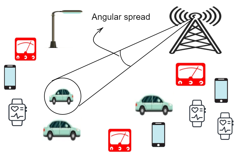
A unique, novel feature of our proposed random access strategy, coined blind goal-oriented detection (BGOD), is that it incorporates all characteristics of B5G requirements in all-in-one package. Our method builds upon the assumption that MIMO channels exhibit angular continuous group sparsity features. This implies that only few number of components in the angular domain contribute to the channel of each UE and the angles of arrival (AoAs) corresponding to each UE lie alongside each other in a group, as shown in Figure 1(a) (the interested reader is referred to [26] for detailed description of this feature). We first design a general optimization problem that promotes the angular group sparsity features of the channels corresponding to all UEs. This optimization problem is highly challenging and costly in terms of computational complexity when the number of UEs is very large (as is the case for massive access in B5G/6G wireless networks), and actually computationally intractable or infeasible in practice. Our first goal is to design a simple reconstruction-free framework that only identifies all active UEs, bypassing the difficult task of data recovery (DR) and CE for massive UEs. To this end, we design a novel goal-oriented optimization problem that does not keep information on the UEs’ messages and complex channel coefficients, but it provides instead a way to obtain a goal-oriented continuous function whose maximum value interestingly reveals the angle information of all active UEs. We then design a clustering algorithm to place these angles into several groups and find the ID of active UEs via their angles. This is indeed the case when UEs are stationary (e.g., smart metering MTC devices) and the angles of each UE, e.g., the line of sight (LoS) angle, are known to the BS prior to the RA process. For the case where UEs are moving or their angles are not known to the BS in advance, we design an alternating minimization (AM) method to recover both the messages and the complex channel coefficients corresponding to active UEs. The ID of each active user is contained in its data payload. By the proposed strategy, the ID and data payloads of active UEs and the channels can be fully obtained blindly.

The novel features and the main contributions of our work are summarized as:

1. 1.

   Massive connectivity. Interestingly, the proposed goal-oriented optimization problem does not depend on the number of total users, whereas the complexity of our clustering scheme does depend on the number of active UEs. Therefore, a massive number of devices with sporadic traffic can access to the network. Actually, the higher the number of antennas at the BS, the more active UEs can access the network. To the best of our knowledge, this is the first work where the RA strategy is independent of the number of devices.

2. 2.

   High reliability. Employing massive number of antennas at the BS and orthogonal preambles at the devices leads to precise detection of the angles and facilitates reliable data recovery. The lower the maximum length of groups (known as angular spread), the fewer observations are required at the BS for exact recovery of angles. Interestingly, devices that selected the same orthogonal preambles (due to limitation in channel coherence time) can still be distinguished by their different angles. The possibility that two active users exist at the same time with the same preamble and with the same continuous angles is very low and can be ignored.

3. 3.

   Low latency. We design an alternating direction method of multipliers (ADMM) in order to directly and rapidly obtain the goal-oriented continuous function by a few measurements obtained at the BS. The proposed algorithm is very fast and may fulfil the low latency requirement of B5G/6G systems. Moreover, the proposed algorithm operates in a blind way, i.e, the BS does not need to use pilots for channel estimation and does not need to coordinate with users in advance. This makes our RA strategy very fast without any extra access latency. Since there are no collisions of active users in our method, there is no need for any contention resolution step. Therefore, as shown in Figure 1(c), the proposed RA strategy is performed in only one step and with very low access delay.

4. 4.

   Limited resources. The goal-oriented feature introduced in this work opens up the possibility of spending as few orthogonal preambles as possible in a blind way, which results in significant resource saving. There is no need to use known pilots for channel estimation and the devices can transmit only their data. This feature is important for MTC/IoT devices, which are battery-operated and operate using limited bandwidth and low power.

The remainder of this paper is structured as follows. Section II introduces the considered wireless system model with its specific features. In Section III, we present the proposed blind goal-oriented RA approach, which consists of four steps: goal-oriented optimization III-A, ADMM III-B, active UE identification III-C, and message recovery III-D. In Section IV we assess the performance of our algorithm and compare it with state-of-the-art RA schemes using numerical experiments. Finally, Section V concludes the paper.

We use boldface lower and uppercase letters for vectors and matrices, respectively. The $i$-th element of a vector $\bm{x}$ and the $(i,l)$ element of a matrix $\bm{X}$ are respectively denoted by $x_{i}$ and $X_{(i,l)}$. The notation $j$ is employed to represent the imaginary unit. The real and imaginary parts of a complex-valued matrix $\bm{A}=\bm{A}^{R}+j\bm{A}^{I}\in\mathbb{C}^{n_{1}\times n_{2}}$ are shown by $\bm{A}^{R}$ and $\bm{A}^{I}$, respectively, and $\overline{\bm{A}}:=\bm{A}^{R}-j\bm{A}^{I}$ denotes the conjugate. For vector $\bm{x}\in\mathbb{C}^{n}$ and matrix $\bm{X}\in\mathbb{C}^{n_{1}\times n_{2}}$, the $\ell_{2}$ norm and Frobenius norm are defined as $\|\bm{x}\|_{2}:=({\sum_{i=1}^{n}|x(i)|^{2}})^{\tfrac{1}{2}}$ $\|\bm{X}\|_{F}:=\sqrt{\sum_{i=1}^{n_{1}}\sum_{j=1}^{n_{2}}|X(i,j)|^{2}}$, respectively. $\bm{X}\succeq\bm{0}$ means that $\bm{X}$ is a positive semidefinite matrix. $\mathcal{P}_{\Omega}(\cdot)$ is a operator transforming an arbitrary matrix to a reduced matrix with rows indexed by $\Omega$. $\langle\bm{A},\bm{B}\rangle:=\sum_{i=1}^{n_{1}}\sum_{l=1}^{n_{2}}A_{i,l}\overline{B}_{i,l}$ is the inner product of two complex-valued matrices $\bm{A}\in\mathbb{C}^{n_{1}\times n_{2}}$ and $\bm{B}\in\mathbb{C}^{n_{1}\times n_{2}}$. The Toeplitz matrix $\mathcal{T}(\bm{v})$ is defined as

where the $(i,l)$-th element is given by $\mathcal{T}(\bm{v})_{(i,l)}=\left\{\begin{array}[]{cc}v_{i-l+1}&i\geq l\\ \overline{v}_{l-i+1}&i<l\end{array}\right\}$. $\bm{1}_{\Omega}$ is a vector of size $\mathbb{R}^{N}$ which has $1$s on the indices corresponding to the set $\Omega$ and zero elsewhere. ${\rm diag}(\bm{x})$ is a diagonal matrix whose main diagonal has elements of $\bm{x}\in\mathbb{R}^{N}$. $\bm{e}_{1}\in\mathbb{R}^{N}$ is the canonical vector whose first element is $1$ and zero elsewhere, i.e., $e_{1}(1)=1,~e_{1}(i)=0,i=2,...,N$. $\bm{x}\odot\bm{y}\in\mathbb{C}^{N}$ is the element-wise operation of two vectors $\bm{x}\in\mathbb{C}^{N}$ and $\bm{y}\in\mathbb{C}^{N}$ and its $i$-th element is given by $x_{i}y_{i}$. The element-wise inequality for two vectors $\bm{x}\in\mathbb{R}^{N}$ and $\bm{y}\in\mathbb{R}^{N}$ is represented by $\bm{x}\geq\bm{y}$ which means $x_{i}\geq y_{i},i=1,...,N$. $\mathds{E}$ and $\mathds{P}$ denote expectation and probability, respectively.

In (5), we have a system of equations with a very large number of unknowns (i.e., $KNT$) and only $MT$ observations at the BS. Leveraging the degrees of freedom of the problem in (5), which is $\sum_{k\in\mathcal{S}_{\rm AU}}(L_{k}+T)$, motivates us to use a general optimization problem that encourages the features corresponding to all UEs simultaneously similar to what $\ell_{0}$ functional offers to encourage sparsity feature in conventional CS. Capitalizing on the results from continuous compressed sensing (CS) (see e.g., [37, 38, 39, 35, 36, 40]), such general optimization framework is as follows:

where $\|\bm{Z}_{k}\|_{\mathcal{A},0}\coloneqq\inf\big\{L_{k}:\bm{Z}_{k}=\sum_{l=1}^{L_{k}}c_{l}^{k}\bm{a}({\theta}_{l}^{k})\bm{\phi}_{k}^{H},c_{l}^{k}>0,\bm{a}(\theta_{l}^{k})\bm{\phi}_{k}^{H}\in\mathcal{A}_{k}\big\}$ is the atomic $\ell_{0}$ function that computes the least number of atoms needed to describe $\bm{Z}_{k}$ by the atoms in the atomic set $\mathcal{A}_{k}$ and $\sum_{k=1}^{K}\|{\bm{Z}_{k}}\|_{\mathcal{A}_{k},0}$ is a function that promotes $\sum_{k=1}^{K}L_{k}$. We reformulate (6) into an equivalent form called LASSO-type and add a regularization term to ensure consistency of the measurements given by:

where $\gamma>0$ is a regularization parameter that makes a balance between the noise energy and the angular sparsity feature with a role similar to $\eta>0$ in (6). Nevertheless, the optimization problem (III-A) is NP-hard and intractable in general. It is therefore beneficial to work with the nearest tractable convex optimization problem whose objective function is a convex relaxation of that in (III-A) and is stated as follows:

where the atomic norm $\|\cdot\|_{\mathcal{A}_{k}}$ is the best convex surrogate for the number of atoms composing $\bm{Z}_{k}$ (i.e., $\|\cdot\|_{\mathcal{A}_{k},0}$) and is defined as the minimum of the $\ell_{1}$ norm of the coefficients forming $\bm{Z}_{k}$:

where ${\rm conv(\mathcal{A})}$ is the convex hull of $\mathcal{A}$. Despite convexity of the objective function in (III-A), it remains computationally intractable due to the continuous nature of the angles $\theta_{k}$s. The objective of this work is to identify the AoAs corresponding to active users. The following theorem provides a novel reconstruction-free optimization problem, which contains only the information of AoAs corresponding to active users and ignores the message information and the channel coefficients corresponding to massive number of UEs. In fact, this theorem provides a goal-oriented framework of solving (III-A), in which the goal is only restricted to active user detection, i.e., finding the AoAs corresponding to the active users. Before stating this theorem, we first need to define the minimal wrap-around distance (also called minimum separation) between angles as

where the absolute value only in the latter relation is evaluated over the unit circle, e.g., $|0.01-0.09|=0.02$.

Discussion: The above theorem shows that all necessary information required for identifying active users is contained in the goal-oriented dual polynomial $\bm{q}_{G}(\theta)$. Figure 2 shows a typical example of the $\ell_{2}$ norm of the goal-oriented function $\|\bm{q}_{G}(\theta)\|_{2}$. The active devices can be identified by finding the angles that maximizes $\|\bm{q}_{G}(\theta)\|_{2}$. The proposed optimization problem (1) is independent of the number of devices $K$ and can be solved for instance using CVX [41] (CVX calls for SDPT3 solvers). To obtain $\|\bm{q}_{G}(\theta)\|_{2}$, we need the matrix dual solution $\bm{V}$. Most of the CVX solvers return the dual variables along with the primal variables. However, solving this optimization problem is highly challenging, in particular for massive MIMO communications where the BS is equipped with a very large number of antennas $N$. Thus, the SDPT3 solver of CVX cannot reach to a solution. In order to solve this this issue, we design a fast ADMM method (see Section III-B), which significantly reduces the computational complexity and is tailored to problems encountered in massive access.

Solving the optimization problem (1) with SDPT3 is prohibitive when $N$ and $T$ are very large. For that, we propose here an ADMM algorithm that can be executed in a significantly faster time. The general idea is to first form an augmented Lagrangian function for the optimization problem and then to split it into a sum of separable functions. In fact, each step of ADMM involves finding a local minimum on a variable [42]. The steps are repeated until some stopping criteria is satisfied. To apply this method, we first find an augmented version of (1) by incorporating an intermediate variable $\bm{\Psi}$ into (1) in order to decouple the semidefinite constraint from the affine constraints. This leads to the following equivalent problem:

The augmented Lagrangian function for (III-B) is given as

where $\rho>0$ is a regularization parameter and $\bm{\Lambda}=\begin{bmatrix}\bm{\Lambda}_{0}&\bm{\Lambda}_{1}\\ \bm{\Lambda}_{1}&\overline{\bm{\Lambda}}\end{bmatrix}$ is the Lagrangian dual multiplier. Denoting the $t$-th step of $\bm{\Psi}$ and $\bm{\Lambda}$ by $\bm{\Psi}^{t}$ and $\bm{\Lambda}^{t}$, ADMM successively updates the following steps to minimize the Lagrangian function $\mathcal{L}_{\rho}$:

where $t$ indicates the iteration number. To make the method practical, we need to obtain efficient implementations for all of the steps. Obviously, the Lagrangian function $L_{\rho}$ is convex with respect to $\bm{Z}$ and $\bm{W}$. Hence, we can obtain closed-form update solutions for $\bm{Z}$ and $\bm{W}$ by setting the partial derivative of $\mathcal{L}_{\rho}$ equal to zero as follows:

which lead to closed-form relations

where $\bm{P}_{\Omega}$ and $\bm{P}_{\Omega}^{{\rm Adj}}$ are matrix forms of the linear operators $\mathcal{P}_{\Omega}$ and $\mathcal{P}^{{\rm Adj}}_{\Omega}$ which by using MATLAB notations are obtained as

in which $\bm{D}={\rm diag}(\bm{1}_{\Omega})\in\mathbb{R}^{N\times N}$. The closed-form expression for $\bm{v}$ is provided in the following lemma:

The update of $\bm{\Psi}$ requires to compute a projection onto the cone of positive semidefinite Hermitian matrices which can be regarded as the most costly part and is provided below:

The relation (25) can be solved by computing the eigenvalue decomposition of $\begin{bmatrix}\mathcal{T}(\bm{v})&\bm{Z}\\ \bm{Z}^{H}&\bm{W}\end{bmatrix}-\frac{\bm{\Lambda}}{\rho}$ and retaining only the directions corresponding to positive eigenvalues. By performing the steps (21), (1), (25) and (18) iteratively, the dual matrix multiplier $\bm{\Lambda}_{1}\in\mathbb{C}^{N\times T}$ is found. However, according to Theorem 1, to achieve the AoAs corresponding to the active users, we need an estimate for the dual matrix $\bm{V}\in\mathbb{C}^{M\times T}$. In the following lemma whose proof is provided in Appendix G, we find a closed-form relation that clearly specifies the connection between these variables.

Once $\mathcal{P}^{{\rm Adj}}(\bm{V})$ is found using Lemma 2, we can use the relation (12) in Theorem 1 to estimate the active angles corresponding to the active devices. Although we have now full access to the angles, there is still ambiguity in which angles corresponds to which active user. Applying a clustering algorithm, we can place angles into several clusters, each of which represents the angles of an active device. If the number of active devices $K_{a}$ is known beforehand (an assumption widely used in the literature, e.g., [12]), the $k$-means clustering algorithm can be employed with known number of clusters. When $K_{a}$ is not known, which seems to be more reasonable in practice, we can use elbow clustering method [43], which chooses the optimal number of clusters by identifying a sharp elbow (knee point) in the graph of explained variations versus clusters. The key idea is that adding another cluster does not provide much better modeling of the angles. The elbow clustering algorithm provides the angles estimate $\{\widehat{\bm{\theta}}^{k}\}_{k=1}^{\widehat{K}_{a}}$ in $\widehat{K}_{a}$ clusters as follows

The number of clusters provides an estimate of $K_{a}$ and the number of angles within the $k$-th cluster gives an estimate of $\widehat{L}_{k}$.

If the devices are stationary and the BS have full information on the angles (for instance only the line of sight (LoS) angle) of each device before random access, then the BS can exactly understand at this stage which device is active and may provide an estimate for $\mathcal{S}_{\rm AU}$, denoted by $\widehat{\mathcal{S}}_{\rm AU}$, and the RA task is finished. If angle information of the devices is not provided or devices do not remain stationary in a known place, the BS can still identify the active users by recovering their unique preambles; this is explained in the next subsection.

To recover the preamble and data of each device, we employ an alternating minimization scheme, in which an initial estimate of $\bm{\phi}_{k}$ is first generated and the following optimization is then solved as a means to find the complex channel amplitudes:

which can be obtained by

where $\bm{A}_{k}:=[\bm{a}(\theta^{k}_{1}),...,\bm{a}(\theta^{k}_{\widehat{L}_{k}})]\in\mathbb{C}^{N\times\widehat{{L}}_{k}}$ and $\bm{\phi}^{\dagger}_{k}$ is the $k$-th column of the pseudo inverse of $\bm{\Phi}:=[\bm{\phi}_{1}^{T},...,\bm{\phi}_{\widehat{K}_{a}}^{T}]^{T}\in\mathbb{C}^{\widehat{K}_{a}\times T}$ denoted by ${\bm{\Phi}}^{\dagger}$.

Having now an estimate of $\widehat{\bm{\alpha}}^{k}$, we can update the estimate $\widehat{\bm{\phi}}_{k}$ by solving

where the non-negative constraint $\bm{\phi}_{k}\geq\bm{0}$ is included to remove any ambiguities caused by multiplications of two elements, as well as to uniquely identify the preamble and data of UEs. The latter optimization problem leads to the following closed-form relation

where $\bm{B}\coloneqq[\mathcal{P}_{\Omega}\bm{A}_{1}\widehat{\bm{\alpha}}^{1},...,\mathcal{P}_{\Omega}\bm{A}_{\widehat{K}_{a}}\widehat{\bm{\alpha}}^{\widehat{K}_{a}}]\in\mathbb{C}^{M\times\widehat{K}_{a}}$ and $(\cdot)_{+}$ keeps the non-negative parts of a matrix as they are and makes zero elsewhere. By performing steps (29) and (31) alternatively, the data and complex channel coefficients are uniquely found within few iterations. Since the transmitted data contains the unique user ID, the active user indices are obtained after recovering the users’ data $\bm{\phi}_{k}$s.

The pseudocode of the proposed method, which summarizes the aforementioned steps, is provided in Algorithm 1.

References

- [1] T. M. Ho, T. D. Tran, T. T. Nguyen, S. Kazmi, L. B. Le, C. S. Hong, and L. Hanzo, “Next-generation wireless solutions for the smart factory, smart vehicles, the smart grid and smart cities,” arXiv preprint arXiv:1907.10102, 2019.
- [2] N. H. Mahmood, H. Alves, O. A. López, M. Shehab, D. P. M. Osorio, and M. Latva-Aho, “Six key features of machine type communication in 6g,” in 2020 2nd 6G Wireless Summit (6G SUMMIT), pp. 1–5, IEEE, 2020.
- [3] M. Hasan, E. Hossain, and D. Niyato, “Random access for machine-to-machine communication in LTE-advanced networks: Issues and approaches,” IEEE communications Magazine, vol. 51, no. 6, pp. 86–93, 2013.
- [4] E. Björnson, E. De Carvalho, J. H. Sørensen, E. G. Larsson, and P. Popovski, “A random access protocol for pilot allocation in crowded massive MIMO systems,” IEEE Transactions on Wireless Communications, vol. 16, no. 4, pp. 2220–2234, 2017.
- [5] O. Y. Bursalioglu, C. Wang, H. Papadopoulos, and G. Caire, “Rrh based massive MIMO with “on the fly” pilot contamination control,” in 2016 IEEE International Conference on Communications (ICC), pp. 1–7, IEEE, 2016.
- [6] J. Kim, G. Lee, S. Kim, T. Taleb, S. Choi, and S. Bahk, “Two-step random access for 5g system: Latest trends and challenges,” IEEE Network, vol. 35, no. 1, pp. 273–279, 2020.
- [7] L. Liu and W. Yu, “Massive connectivity with massive MIMO—part i: Device activity detection and channel estimation,” IEEE Transactions on Signal Processing, vol. 66, no. 11, pp. 2933–2946, 2018.
- [8] L. Liu and W. Yu, “Massive connectivity with massive MIMO—part ii: Achievable rate characterization,” IEEE Transactions on Signal Processing, vol. 66, no. 11, pp. 2947–2959, 2018.
- [9] Z. Chen, F. Sohrabi, and W. Yu, “Sparse activity detection in multi-cell massive MIMO exploiting channel large-scale fading,” IEEE Transactions on Signal Processing, 2021.
- [10] K. Senel and E. G. Larsson, “Grant-free massive MTC-enabled massive MIMO: A compressive sensing approach,” IEEE Transactions on Communications, vol. 66, no. 12, pp. 6164–6175, 2018.
- [11] S. Haghighatshoar, P. Jung, and G. Caire, “Improved scaling law for activity detection in massive MIMO systems,” in 2018 IEEE International Symposium on Information Theory (ISIT), pp. 381–385, IEEE, 2018.
- [12] M. Ke, Z. Gao, Y. Wu, X. Gao, and R. Schober, “Compressive sensing based adaptive active user detection and channel estimation: Massive access meets massive mimo,” IEEE Transactions on Signal Processing, 2020.
- [13] H. Djelouat, M. Leinonen, L. Ribeiro, and M. Juntti, “Joint user identification and channel estimation via exploiting spatial channel covariance in mmtc,” IEEE Wireless Communications Letters, vol. 10, no. 4, pp. 887–891, 2021.
- [14] A. Fengler, G. Caire, P. Jung, and S. Haghighatshoar, “Massive MIMO unsourced random access,” arXiv preprint arXiv:1901.00828, 2019.
- [15] A. Fengler, O. Musa, P. Jung, and G. Caire, “Pilot-based unsourced random access with a massive MIMO receiver, interference cancellation, and power control,” IEEE Journal on Selected Areas in Communications, 2022.
- [16] X. Xie, Y. Wu, J. An, J. Gao, W. Zhang, C. Xing, K.-K. Wong, and C. Xiao, “Massive unsourced random access: Exploiting angular domain sparsity,” IEEE Transactions on Communications, 2022.
- [17] L. Liu, E. G. Larsson, W. Yu, P. Popovski, C. Stefanovic, and E. De Carvalho, “Sparse signal processing for grant-free massive connectivity: A future paradigm for random access protocols in the internet of things,” IEEE Signal Processing Magazine, vol. 35, no. 5, pp. 88–99, 2018.
- [18] Z. Chen, F. Sohrabi, Y.-F. Liu, and W. Yu, “Covariance based joint activity and data detection for massive random access with massive MIMO,” in ICC 2019-2019 IEEE International Conference on Communications (ICC), pp. 1–6, IEEE, 2019.
- [19] Z. Chen, F. Sohrabi, and W. Yu, “Sparse activity detection for massive connectivity,” IEEE Transactions on Signal Processing, vol. 66, no. 7, pp. 1890–1904, 2018.
- [20] A. Afshar, V. Tabataba Vakili, and S. Daei, “Active user detection and channel estimation for spatial-based random access in crowded massive MIMO systems via blind super-resolution,” IEEE Signal Processing Letters, 2022.
- [21] H. Huang, J. Yang, H. Huang, Y. Song, and G. Gui, “Deep learning for super-resolution channel estimation and doa estimation based massive MIMO system,” IEEE Transactions on Vehicular Technology, vol. 67, no. 9, pp. 8549–8560, 2018.
- [22] Y. Ahn, W. Kim, and B. Shim, “Active user detection and channel estimation for massive machine-type communication: Deep learning approach,” IEEE Internet of Things Journal, 2021.
- [23] H. S. Jang, H. Lee, T. Q. Quek, and H. Shin, “Deep learning-based cellular random access framework,” IEEE Transactions on Wireless Communications, vol. 20, no. 11, pp. 7503–7518, 2021.
- [24] J. Ding, D. Qu, and J. Choi, “Analysis of non-orthogonal sequences for grant-free RA with massive MIMO,” IEEE Transactions on Communications, vol. 68, no. 1, pp. 150–160, 2019.
- [25] Z. Ding, R. Schober, P. Fan, and H. V. Poor, “Simple semi-grant-free transmission strategies assisted by non-orthogonal multiple access,” IEEE Transactions on Communications, vol. 67, no. 6, pp. 4464–4478, 2019.
- [26] X. Lin, S. Wu, C. Jiang, L. Kuang, J. Yan, and L. Hanzo, “Estimation of broadband multiuser millimeter wave massive MIMO-OFDM channels by exploiting their sparse structure,” IEEE Transactions on Wireless Communications, vol. 17, no. 6, pp. 3959–3973, 2018.
- [27] X. Shao, X. Chen, D. W. K. Ng, C. Zhong, and Z. Zhang, “Cooperative activity detection: Sourced and unsourced massive random access paradigms,” IEEE Transactions on Signal Processing, vol. 68, pp. 6578–6593, 2020.
- [28] S. Haghighatshoar, P. Jung, and G. Caire, “A new scaling law for activity detection in massive MIMO systems,” arXiv preprint arXiv:1803.02288, 2018.
- [29] Z. Chen, F. Sohrabi, Y.-F. Liu, and W. Yu, “Phase transition analysis for covariance based massive random access with massive MIMO,” IEEE Transactions on Information Theory, 2021.
- [30] L. You, X. Gao, X.-G. Xia, N. Ma, and Y. Peng, “Pilot reuse for massive MIMO transmission over spatially correlated rayleigh fading channels,” IEEE Transactions on Wireless Communications, vol. 14, no. 6, pp. 3352–3366, 2015.
- [31] W. U. Bajwa, J. Haupt, A. M. Sayeed, and R. Nowak, “Compressed channel sensing: A new approach to estimating sparse multipath channels,” Proceedings of the IEEE, vol. 98, no. 6, pp. 1058–1076, 2010.
- [32] J. Zhang, X. Yuan, and Y.-J. A. Zhang, “Blind signal detection in massive mimo: Exploiting the channel sparsity,” IEEE Transactions on Communications, vol. 66, no. 2, pp. 700–712, 2017.
- [33] J. Ma, S. Zhang, H. Li, F. Gao, and S. Jin, “Sparse bayesian learning for the time-varying massive MIMO channels: Acquisition and tracking,” IEEE Transactions on Communications, vol. 67, no. 3, pp. 1925–1938, 2018.
- [34] V. Chandrasekaran, B. Recht, P. A. Parrilo, and A. S. Willsky, “The convex geometry of linear inverse problems,” Foundations of Computational mathematics, vol. 12, no. 6, pp. 805–849, 2012.
- [35] E. J. Candès and C. Fernandez-Granda, “Towards a mathematical theory of super-resolution,” Communications on pure and applied Mathematics, vol. 67, no. 6, pp. 906–956, 2014.
- [36] G. Tang, B. N. Bhaskar, P. Shah, and B. Recht, “Compressed sensing off the grid,” IEEE transactions on information theory, vol. 59, no. 11, pp. 7465–7490, 2013.
- [37] S. Sayyari, S. Daei, and F. Haddadi, “Blind two-dimensional super-resolution in multiple-input single-output linear systems,” IEEE Signal Processing Letters, 2020.
- [38] S. Bayat and S. Daei, “Separating radar signals from impulsive noise using atomic norm minimization,” IEEE Transactions on Circuits and Systems II: Express Briefs, 2020.
- [39] S. Daei, F. Haddadi, and A. Amini, “Living near the edge: A lower-bound on the phase transition of total variation minimization,” IEEE Transactions on Information Theory, vol. 66, no. 5, pp. 3261–3267, 2019.
- [40] C. Fernandez-Granda, “Super-resolution of point sources via convex programming,” Information and Inference: A Journal of the IMA, vol. 5, no. 3, pp. 251–303, 2016.
- [41] M. Grant and S. Boyd, “Cvx: Matlab software for disciplined convex programming, version 2.1,” 2014.
- [42] S. Boyd, N. Parikh, and E. Chu, Distributed optimization and statistical learning via the alternating direction method of multipliers. Now Publishers Inc, 2011.
- [43] F. Liu and Y. Deng, “Determine the number of unknown targets in open world based on elbow method,” IEEE Transactions on Fuzzy Systems, vol. 29, no. 5, pp. 986–995, 2020.
- [44] B. Dumitrescu, Positive Trigonometric Polynomials and Signal Processing Applications. Springer, 2017.
- [45] Y. Chi, “Guaranteed blind sparse spikes deconvolution via lifting and convex optimization,” IEEE Journal of Selected Topics in Signal Processing, vol. 10, no. 4, pp. 782–794, 2016.
- [46] S. P. Boyd and L. Vandenberghe, Convex optimization. Cambridge university press, 2004.