Planck Stars from a Scale-dependent Gravity theory

In many of the existing approaches to quantum gravity (for an incomplete list see e.g. QG1; QG2; QG3; QG4; QG6; QG8; QG9 and references therein) the fundamental parameters that enter the action, such as Newton’s constant, electromagnetic coupling, the cosmological constant etc., become scale dependent quantities. This looks quite natural, since scale dependence at the level of the effective action is a generic feature of ordinary quantum field theory. In particular, in theories of gravity, the scale dependence is expected to modify the horizon, the thermodynamics, the quasinormal modes spectra of classical black hole backgrounds Koch:2016uso; Rincon:2017goj; Contreras:2017eza; Rincon:2018sgd; Contreras:2018dhs; Rincon:2019cix; Contreras:2018gpl. In the large class of approaches based on scale-dependent gravity (SDG), among the theories beyond classical general relativity (GR), we find also the particular method usually known as asymptotically safe gravity (ASG) Bonanno:2000ep; Bonanno:2001xi; Reuter:2003ca; Platania:2020lqb; Bonanno:2002zb; Bonanno:2001hi; Liu:2018hno; Hindmarsh:2012rc; Platania:2019kyx; Moti:2018uvl; Koch:2013owa; Koch:2014cqa; Saueressig:2015xua; Bonanno:2016dyv; chinosII; Li:2013kkb. In this scenario the Newton’s constant $G$ is actually seen as a ”running” Newton’s coupling $G(k)$, which is constructed by integrating the differential equation for the beta function of the gravitational coupling. Therefore $G$ depends on some arbitrary renormalization energy scale $k$. Furthermore, in concrete black hole models, usually a link between the energy scale $k$ and the radial coordinate $r$ is established. Finally, the composite function $G(k(r))$ is inserted back into the classical black hole solution. A modified lapse function is thus obtained, and these modified black hole metrics are thought to automatically incorporate and describe the effects of quantum gravity. Other different black hole metrics, in particular metrics not affected by a central singularity, can be found e.g. in Refs. bardeen; hayward; flachi; frolov; BS2, although those examples may not be directly connected with a SDG program.
Generic examples of SDG theories, in particular scale-dependent black hole solutions, can be found in literature, see for example Refs. Koch:2016uso; Contreras:2017eza; Contreras:2018gpl. As for the subclass ASG, a specific well known example (see e.g. Refs. Bonanno:2000ep; LS) is defined by the ”running” Newton’s coupling $G(k)$ and function $k(r)$

$\displaystyle G(k)=\frac{G}{1+\tilde{\omega}Gk^{2}/\hbar}\ \quad\quad{\rm with}\quad\quad k(r)=\hbar\left(\frac{r+\gamma GM}{r^{3}}\right)^{1/2}$

(1)

where we take the conventions $c=k_{B}=1$ and we retain $\hbar$. Here $\tilde{\omega}$ and $\gamma$ are dimensionless numerical parameters. Combined together the above functions yield the scale-dependent Newton’s constant

$\displaystyle G(r)=\frac{Gr^{3}}{r^{3}+\tilde{\omega}G\hbar\left(r+\gamma GM\right)}\,.$

(2)

In the context of ASG literature, the parameter $\tilde{\omega}$ is always assumed to be positive, $\tilde{\omega}>0$. In fact, considering the running Newton’s coupling $G(k)$ in Eq.(1), we see that $dG/dk<0$ only if $\tilde{\omega}>0$. In other words, in order to keep gravity ”asymptotically safe” from divergences, we need to have not only $G(k)\to 0$ for $k\to\infty$, but also $G(k)\geq 0$ and finite for any $k\geq 0$. Therefore, only when $\tilde{\omega}>0$ we are properly in the realm of an Asymptotically Safe Gravity theory.

On the contrary, if we allow $\tilde{\omega}<0$, then $G(k)$ diverges for $k\sim k_{Planck}$, becomes negative for $k>k_{Planck}$ and $G(k)\to 0^{-}$ when $k\to\infty$. This behavior of $G(k)$ is clearly outside the specific spirit of ASG theory. Nevertheless, a theory with $\tilde{\omega}<0$ can still be classified as a scale-dependent gravity (SDG) theory. In the following we will see that this is actually our present case.

A different, well known research line, pursued by John Donoghue and other authors Duff; donoghue; hamber; kiril; dono2; kiril2; dono3; donoASP; frob, considers the reformulation of General Relativity as an effective quantum field theory of gravity at low energies. Along the years, these authors established a solid prediction of the quantum corrections to the Schwarzschild metric, and therefore to the Newtonian potential, at least at the first order in $\hbar$. According to a vast literature, a way to determine the free parameters appearing in a SDG theory, and in particular in a ASG-metric (see e.g. Refs. Bonanno:2000ep; Bonanno:2001xi; Reuter:2003ca; Platania:2020lqb; Bonanno:2002zb; Bonanno:2001hi; Liu:2018hno; Hindmarsh:2012rc; Platania:2019kyx; Moti:2018uvl; Koch:2013owa; Koch:2014cqa; Saueressig:2015xua; Bonanno:2016dyv; chinosII; Li:2013kkb), consists in comparing the effective Newtonian potential predicted by the SDG/ASG approach with the one computed in the framework of GR as an effective QFT. By following that path, we are led to investigate, for the first time, a negative value for the parameter $\tilde{\omega}$, unlike previous early studies (see e.g. Refs. Bonanno:2000ep; Koch:2014cqa) ¹¹ 1 Here we should at least mention the ongoing lively debate among the communities working on GR as an Effective Field Theory (EFT), and those on the ASG approach. The focus is about ”if” and ”to what extent” the results obtained on ASG-improved metrics by the ASG community can be compared with the results on the quantum corrected metrics obtained by the GR-EFT community (see e.g. Refs. donoASP; BonannoFP). Here, of course, we cannot enter in details. However, after a long period during which this matching has been carried out almost routinely, without particular problems, quite recently, doubts have been risen about the effective comparability of the calculations of the two communities, and the conceptual correctness of such comparison. In particular, it would seem that the two different frameworks effectively consider, and implement, different classes of Feynman diagrams in order to get their final (quantum corrected) metric expressions. Of course, including or not including certain subclasses of diagrams could change the sign of the parameters involved. Thus, the overall feeling is that at present a comparison between GR-EFT and ASG results could even be not well grounded, and in any case the available calculations are not yet able to clarify the situation. This however looks to us as an even stronger motivation to explore the physical consequences of a negative $\tilde{\omega}$ parameter..

As said above, this classifies our approach outside a standard ASG theory, instead closer to a more general SDG theory. Quite surprisingly, we will see that the negative $\tilde{\omega}$ leads directly, without further assumptions, to a specific metric which is able to describe important features of the so called Planck stars. It is remarkable that, while Planck stars were introduced in Ref. RovelliPS on the grounds of plausible, general physical considerations, here on the contrary they appear as a possible direct consequence of a Scale-Dependent Gravity approach.

The paper is organized as follows. In the next Section we shortly recall the main results leading to a SDG/ASG-modification of the Schwarzschild metric. In Section III we give a precise evaluation of the SDG/ASG parameters. Section IV is devoted to discuss the features of the SDG-modified Schwarzschild metric, and then Section V discusses the ”prediction” of the Planck star model. In Sections VI, VII, VIII, IX we study, respectively, temperature, specific heat, emission rate equation, and thermodynamic entropy of this SDG-modified Schwarzschild/Planck star metric. The last Section contains some quick hints to the phenomenology of these objects (and related references), and the conclusions.

Here we work in units where $c=k_{B}=1$, and the Planck length $\ell_{P}$ is defined as $G\hbar=\ell_{P}^{2}$. Then of course the Planck mass $m_{P}$ satisfies $2Gm_{P}=\ell_{P}$ and $\hbar=2m_{P}\ell_{P}$.

As we said in Sec.II, the SDG/ASG-modified Newtonian potential can be obtained from the standard Newton formula

$\displaystyle V(r)=-\frac{GMm}{r}$

(9)

by simply replacing the experimentally observed Newton constant $G$ with the running coupling $G(r)$ given in Eq.(2). Thus we get

$\displaystyle V^{SDG}(r)=-\frac{G(r)Mm}{r}=-\frac{G\,M\,m\,r^{2}}{r^{3}+\tilde{\omega}\,G\,\hbar\,(r+\gamma GM)}\,,$

(10)

which can be expanded for large $r$ as

$\displaystyle V^{SDG}(r)=-\frac{GMm}{r}\left[1-\frac{\tilde{\omega}G\hbar}{r^{2}}-\frac{\gamma\tilde{\omega}G^{2}\hbar M}{r^{3}}+{\cal O}\left(\frac{G^{2}\hbar^{2}}{r^{4}}\right)\right]\,.$

(11)

Clearly, the corrections to the standard Newtonian potential predicted by the SDG/ASG approach are all of quantum nature. This is suggested by the presence of $\hbar$ in each term of correction. In fact, there are no correction terms of classical origin, coming from some kind of post-Newtonian approximation. On the other hand, corrections of quantum origin to the classical Newtonian potential have been elaborated by several researchers Duff; donoghue; hamber; kiril; dono2; kiril2; dono3; donoASP; frob in the last three decades or so. In particular, it was pointed out by Donoghue donoghue; dono2 that the standard perturbative quantization of Einstein gravity leads to a well defined, finite prediction for the leading large distance quantum correction to Newtonian potential (the Effective Field Theory approach mentioned in the Introduction). The numerical coefficients of the quantum expansion have undergone a certain evolution over the years hamber; kiril, but the result today accepted by the community dono2; kiril2 reads

$\displaystyle V^{QGR}(r)\ =\ -\frac{GMm}{r}\left[1\ +\ \frac{41}{10\pi}\frac{G\hbar}{r^{2}}\ +\ \dots\right]\,.$

(12)

This is an expansion at first order in $\hbar$ (and at second order in $1/r$), where the first correction term represents a genuine quantum correction proportional to $\hbar$.

The comparison of the two expansions (11) and (12) allows us to fix the parameter $\tilde{\omega}$, which results to be

$\displaystyle\tilde{\omega}=-\frac{41}{10\pi}\,.$

(13)

The parameter $\gamma$ cannot be fixed by these considerations. To this aim, we refer the reader to the arguments originally developed in Ref.Bonanno:2000ep, and then taken up also by other authors (e.g.Koch:2014cqa). Those classical general relativistic arguments fix $\gamma=9/2$. Different kind of considerations, based on the generalized uncertainty principle (see Ref. LS; see also Refs. GUP), lead to the value $\gamma=0$. In this paper we will assume always $\gamma\geq 0$, and in some specific cases we shall comment on the special value $\gamma=0$. However, most of the results will be qualitatively the same for all $\gamma>0$.

As we said in footnote 1, the last couple of years have witnessed the raising of some doubts against the conceptual correctness of a comparison between the SDG/ASG-modified Newtonian potential (11), with the GR-EFT quantum corrected Newtonian potential (12). Without supporting here one side or the other of this not yet settled down question, it is however perfectly legitimate to explore the physical consequences of the case $\tilde{\omega}<0$, as on the other hand the above Eq.(13) strongly suggests.

We emphasize that the sign of $\tilde{\omega}$ is crucial for the physics of SDG-modified black hole. In the standard, strict, ASG approach, only metrics with $\tilde{\omega}>0$ have been studied. This choice of course has implied black holes where the central singularity is wiped out, in favour of a De Sitter or an Anti De Sitter core, as can be easily inferred from Eqs.(4)(6), and is also widely discussed in the above References. In the next sections, on the contrary, starting from a more general SDG point of view, we shall explore metrics with a negative $\tilde{\omega}$. This choice, as we will see, will have deep consequences on the structure and the physics of the black hole metric (4) considered ²² 2 From a historical point of view, it is interesting to note that, until quite recently, many authors of ASG community (e.g.Bonanno:2000ep; Koch:2014cqa; Saueressig:2015xua), in order to fix the $\tilde{\omega}$ parameter, have relied on a direct comparison between the two expressions (11) and (12). The sign of the $\tilde{\omega}$ parameter has therefore changed according to the sign of the first order correction term in $\hbar$ in the expansion (12). For example, Duff, in his first calculation Duff of 1974 obtained an expansion of the same kind of (12), with a positive coefficient of the $\hbar$ term (and therefore a negative $\tilde{\omega}$). The ASG community has instead actually considered, until few yars ago, the early calculations performed by Donoghue and others donoghue; hamber in the period 1994-1995, where the $\hbar$ coefficient obtained was negative. As a consequence, the ASG authors got a positive value of $\tilde{\omega}$. However, during the years, the analytical techniques used in GR as an effective QFT have been refined, and the results now accepted by the GR-EFT community are those expressed, initially, in Refs.dono2; kiril2, and then confirmed in Refs.dono3, as well as in the very recent Ref.frob. All these results coherently point to a positive $\hbar$ coefficient in the expansion (12) (and hence to a negative value of $\tilde{\omega}$, if the above comparison is effectively considered)..

The key suggestion coming from the previous Section is to consider the possibility of a negative $\tilde{\omega}$. This, as we will see, represents a major change in respect to others modified (but regular) Schwarzschild metrics present in literature Contreras:2017eza; Contreras:2018gpl; Bonanno:2000ep; hayward; flachi; frolov. Instead, some contact with our results can be found in Ref. Bargueno:2016qhu, although there the authors don’t deal with SDG models. So, according to the previous section, we consider here the case

$\displaystyle\tilde{\omega}<0\ \Rightarrow\ \tilde{\omega}=-|\tilde{\omega}|\,;\quad\quad\quad\gamma>0\,.$

(14)

The lapse function (4) can therefore be written as

$\displaystyle F(r)=1-\frac{2GMr^{2}}{r^{3}-|\tilde{\omega}|G\hbar(r+\gamma GM)}\,.$

(15)

While for $\tilde{\omega}>0$ the lapse (4) is regular everywhere when $r>0$ (see e.g. Ref. Bonanno:2000ep), here, with $\tilde{\omega}<0$, the scenario is very different. First, we notice that the behavior of $F(r)$ at $r\to\infty$ remains that described by Eq.(5), namely a standard Schwarzschild metric for large $r$. At $r\to 0$ we have an Anti-DeSitter core, namely $F(r)\simeq 1+2r^{2}/(|\tilde{\omega}|\gamma G\hbar)$. But now the denominator $D(r)$ appearing in (15) can develop zeros. Luckly, a simple graphical analysis is sufficient to clarify the situation. In Fig.1, we compare the two lines

	$\displaystyle y_{1}$	$\displaystyle=$	$\displaystyle r^{3}$
	$\displaystyle y_{2}$	$\displaystyle=$	$\displaystyle|\tilde{\omega}|G\hbar(r+\gamma GM)$		(16)

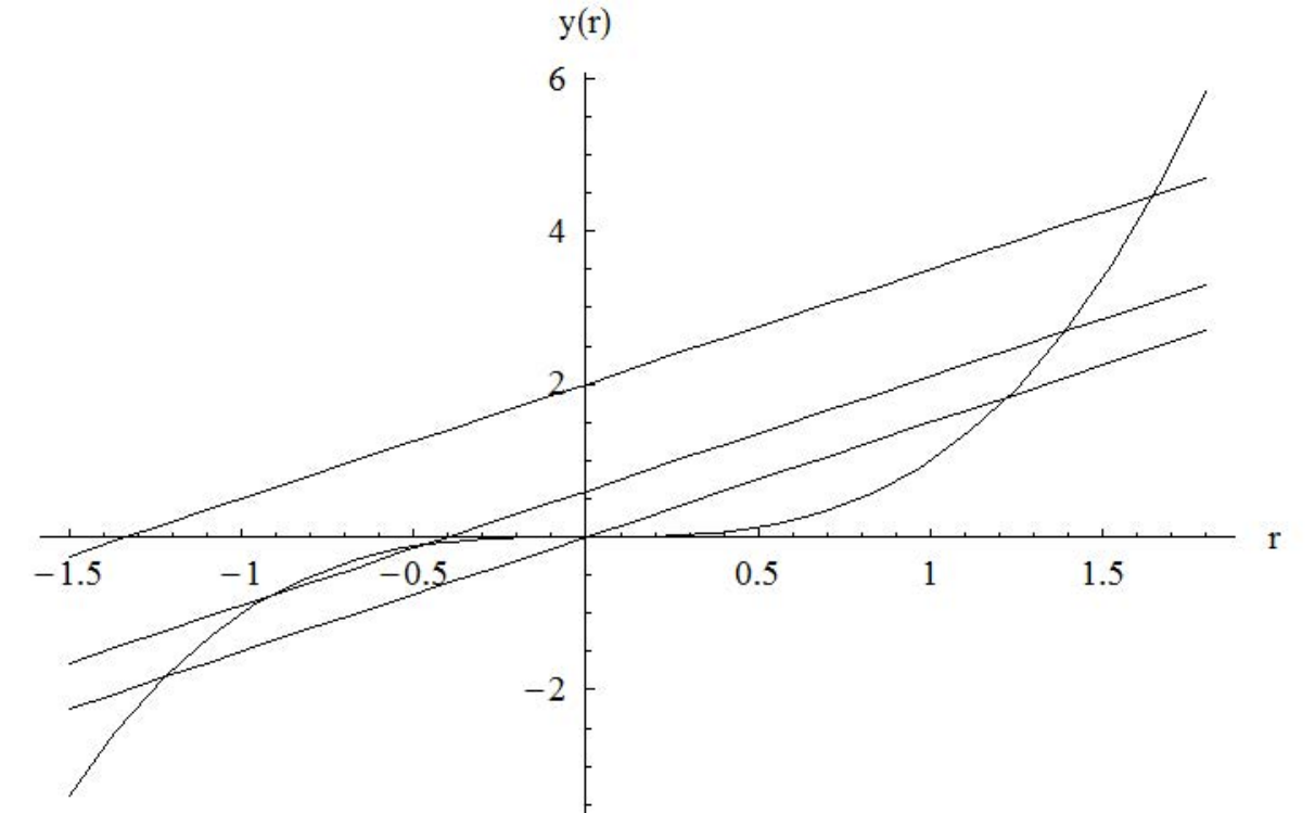
for various values of $M>0$, the mass of the central body. As we see, since $D=y_{1}-y_{2}$, there is always only one single zero for $D(r)$ when $r>0$, let’s call it $r_{0}$. So

	$\displaystyle D(r)$	$\displaystyle>$	$\displaystyle 0\quad{\rm for}\quad r>r_{0}$
	$\displaystyle D(r)$	$\displaystyle=$	$\displaystyle 0\quad{\rm for}\quad r=r_{0}$
	$\displaystyle D(r)$	$\displaystyle<$	$\displaystyle 0\quad{\rm for}\quad 0<r<r_{0}$

In the unphysical region $r<0$, $D(r)$ can develop two distinct zeros, or two coincident zeros, or no real zeros at all. On the ground of the above situation, we can develop a straightforward analysis of the function $F(r)$, valid for any $M>0$:

	$\displaystyle\lim_{r\to+\infty}F(r)=1^{-}\,;\quad\lim_{r\to r_{0}^{+}}F(r)=1-\frac{2GMr_{0}^{2}}{0^{+}}=-\infty\,;$
	$\displaystyle\lim_{r\to r_{0}^{-}}F(r)=1-\frac{2GMr_{0}^{2}}{0^{-}}=+\infty\,;\quad\lim_{r\to 0^{+}}F(r)=1^{+}\,;$
	$\displaystyle F(r)\sim 1+\frac{2r^{2}}{|\tilde{\omega}|\gamma G\hbar}\quad{\rm for}\quad r\sim 0\,;\quad F^{\prime}(r)=\frac{2GM(r^{4}+|\tilde{\omega}|G\hbar r^{2}+2|\tilde{\omega}|\gamma G^{2}M\hbar r)}{(r^{3}-|\tilde{\omega}|G\hbar r-|\tilde{\omega}|\gamma G^{2}\hbar M)^{2}}>0\quad{\rm for}\quad r>0$

The information collected above allows us to draw a general graph (Fig.2) of the lapse function $F(r)$ in the region $r>0$, valid for any $\gamma>0$ and of course $M>0$.

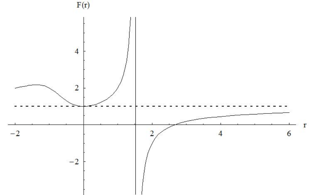
As we see, there is one single positive zero $r=r_{h}$ of $F(r)$, which is the horizon of the SDG-modified black hole metric (15). There is also an essential singularity at $r=r_{0}>0$. The most relevant difference with the standard Schwarzschild metric is the fact that the essential (ineliminable) singularity is at $r_{0}>0$, instead of being at $r_{0}=0$. It is also clear that it is always $r_{0}<r_{h}$, for any $M>0$. So the singularity is always protected by the event horizon. The singularity is never naked, in full accordance with the Cosmic Censorship Conjecture.

We now examine the asymptotic behavior of the horizon $r_{h}$ and of the singularity $r_{0}$ in the physical relevant limits of large $M$ and small $M$.

It is of the greatest interest to examine the core of the black hole metric we obtained. For masses $M$ larger than the Planck mass $m_{p}$, $M\gg m_{p}$, the central hard singularity is located at $r=r_{0}$, and it has, in fact, a finite positive size $r_{0}\simeq(\gamma|\tilde{\omega}|G^{2}\hbar M)^{1/3}>0$, contrary to what happens in the standard Schwarzschild black hole, where the singularity is point-like. Observe that this finite size is completely of quantum origin: in fact, $r_{0}\to 0$ if we take the classical limit $\hbar\to 0$.

But most importantly, if we presume that the whole collapsing mass $M$ is concentrated into the central hard sphere of radius $r_{0}$, then we can compute the (non covariant) volume of this sphere, and hence the density of this matter (as seen by an observer at infinity), which will result to be finite, and precisely

$\displaystyle r_{0}=(\gamma|\tilde{\omega}|\ell_{P}^{2}GM)^{1/3}\ =\ (\gamma|\tilde{\omega}|/2)^{\frac{1}{3}}\left(\frac{M}{m_{p}}\right)^{\frac{1}{3}}\ell_{P}\ \quad\ \Rightarrow\ \quad\ \varrho=\frac{M}{V_{core}}=\frac{3}{2\pi}\frac{m_{p}}{\gamma|\tilde{\omega}|\ell_{P}^{3}}\simeq\frac{m_{p}}{2\gamma|\tilde{\omega}|\ell_{P}^{3}}=\frac{\varrho_{Planck}}{2\gamma|\tilde{\omega}|},$

(38)

where we used the definitions $G\hbar=\ell_{P}^{2}$, $2Gm_{p}=\ell_{P}$, and

$\displaystyle\varrho_{Planck}=\frac{m_{p}}{\ell_{P}^{3}}\,.$

(39)

So the central hard kernel of our black hole results to have a finite size, and a density of the order of the Planck density. These are exactly the characteristics of the so called Planck stars, first proposed in Ref. RovelliPS, on the ground of general qualitative considerations. Many of the general properties described in RovelliPS (see also Ref. BonannoCasadio) can now be repeated for our black hole. The finite positive size of the central core, being of pure quantum origin, is presumably due to the action of the Heisenberg uncertainty principle, which prevents matter to be arbitrarily concentrated into a geometrical point of size zero. The central kernel can presumably keep trace of all the information swallowed by the black hole: we see here a possible way out of the information paradox. Of course, all the above considerations make sense only for $\gamma>0$ strictly.

The original proposal RovelliPS contains a certain amount of qualitative considerations, including an educated guess on the form of the metric able to describe a Planck star. Such metric was initially chosen to be the Hayward metric hayward

$\displaystyle F(r)=1-\frac{2GMr^{2}}{r^{3}+2GML^{2}}$

(40)

where $L$ is a parameter with dimensions of a length. No particularly compelling argument, from the physical point of view, was exhibited for that choice, with the exception, perhaps, that the Hayward metric is a well known example of singularity-free metric. For large $M$ the metric (40) develops two horizons, one inner

$\displaystyle r_{-}\ \simeq\ L\ +\ \frac{L^{2}}{4GM}\,,$

(41)

and one outer

$\displaystyle r_{+}\ \simeq\ 2GM\ -\ \frac{L^{2}}{2GM}.$

(42)

However, no specific indication is contained in the Hayward metric (40) about the size of the hard kernel of a Planck star. Even identifying such hard kernel size with $r_{-}$, certainly it does not increase in size with $M$, as instead Eq.(38) suggests for $r_{0}$ (compare with Eq.(41)). Even worse, the Hayward metric per se is unable to mimic the well established quantum correction to the Newtonian potential dono2 that occurs at low energies. This is due to the lack of a term $1/r^{3}$ in the expansion of the metric (40). The authors of Ref. delorenzo found a smart way to cure this shortcoming, but at the price of introducing a further metric function $H(r)$, determined through a bunch of additional constraints, so that their ”modified Hayward” metric now reads

$\displaystyle ds^{2}=-\ H(r)F(r)dt^{2}+\frac{1}{F(r)}dr^{2}+r^{2}d\Omega^{2}\,,\quad{\rm with}\quad H(r)=1-\frac{\beta GM\alpha}{\alpha r^{3}+\beta GM}\,,$

(43)

where $\beta$ is a parameter that in Ref.delorenzo plays the rôle of our $|\tilde{\omega}|$. The above metric ⁴⁴ 4 A further requirement imposed by the authors on the function $H(r)$ is that $H(r)$ should allow for a time delay between a clock sitting at the center of the collapsed object ($r=0$), and a clock at infinity (put a clock at $r=0$ is in principle conceivable, just because the Hayward metric is regular at $r=0$). To get this, authors demand that $H(r=0)=1-\alpha$. They justify this further request by saying that ”is a physically unmotivated restriction” to leave $H(0)=1$. In any case, we do not have this kind of problem with the SDG metric (15), since the center $r=0$ cannot be reached, being protected by the singularity at $r=r_{0}>0$. finally contains the $1/r^{3}$ term necessary to mimic the Donoghue modified Newtonian potential dono2 for large $r$.
Although smart and working, the above solution is undeniably contorted and intricate. On the contrary, within the formalism of the ’renormalization improved’ and ’running’ coupling constants, the mathematical structure of the metric is dictated by the general properties of the SD/AS Gravity, and its lapse function (15) results clearly simpler than the above product $H(r)F(r)$. Our SDG metric (15) already contains the right terms to match, at large distances, the quantum corrected Newtonian potential. Moreover, and this is quite astonishing, by simply imposing that match, the final form of the metric is uniquely fixed, and it automatically displays the correct size of the central hard kernel of the Planck star.

In the following, we shall therefore study the thermodynamic properties of the metric (15).

According to the celebrated works of Hawking (see e.g. Ref. Hawking), a generic Lorentzian black hole metric as (3) with a lapse function $F(r)$ bearing an horizon (namely a simple zero at some $r=r_{h}$, with $F(r_{h})=0,F^{\prime}(r_{h})\neq 0$), displays on the horizon a Hawking-Bekenstein temperature given by

$\displaystyle T_{BH}=\frac{\hbar}{4\pi}F^{\prime}(r_{h})\,.$

(44)

Therefore, reminding $G\hbar=\ell_{P}^{2}$ and $|\tilde{\omega}|\ell_{P}^{2}=r_{c}^{2}$, from (15) we can compute,

$\displaystyle\frac{4\pi}{\hbar}T\ =\ F^{\prime}(r)\ =\ 2GMr\,\frac{r^{3}+r_{c}^{2}r+2\gamma GMr_{c}^{2}}{(r^{3}-r_{c}^{2}r-\gamma GMr_{c}^{2})^{2}}$

(45)

where we take $r=r_{h}$, namely $r$ should satisfy the identity $F(r)=r^{3}-2GMr^{2}-r_{c}^{2}r-\gamma GMr_{c}^{2}=0$.
We can use this to semplify $r^{3}-r_{c}^{2}r-\gamma GMr_{c}^{2}=2GMr^{2}$, and get

$\displaystyle F^{\prime}(r)\ =\ \frac{1}{2GM}\left(1\ +\ \frac{r_{c}^{2}}{r^{2}}\ +\ \frac{2\gamma GMr_{c}^{2}}{r^{3}}\right)\,.$

(46)

The above expression is exact. Now we study its limits, namely the limits of $T(M)$ for $M$ large and for $M$ small.

Repeating twice the procedure which led us to (20), for $M\to\infty$, we can arrive to write the expansion of $r_{h}(M)$ to the third order in $1/M$

$\displaystyle r\ =\ r_{h}\ \simeq\ 2GM\ +\ \frac{(\gamma+2)r_{c}^{2}}{4GM}\ +\ \frac{(\gamma+2)r_{c}^{4}}{16G^{3}M^{3}}\ +\ \dots$

(47)

Inserting this back into (46) we get finally

$\displaystyle\frac{4\pi}{\hbar}T(M)\ =\ F^{\prime}(r)\ =\ \frac{1}{2GM}\left[1+\frac{\gamma+1}{4}\left(\frac{r_{c}}{GM}\right)^{2}-\frac{(\gamma+2)(3\gamma+2)}{32}\left(\frac{r_{c}}{GM}\right)^{4}+\dots\right]\,.$

(48)

We recover here the standard behavior $T_{BH}=\hbar/8\pi GM$ of the BH temperature for large $M$, when our black hole looks even more like a Schwarzschild one. Moreover, notice that the horizon mass function (35) is an odd function $M(r_{h})$, therefore its inverse $r_{h}(M)$ is an odd function, and its expansion can hence contain odd powers of $M$ only, as in fact results in Eq.(47). Besides, the expression in round brackets in (46) must be an even function of $M$, since $r_{h}(M)$ is odd, and therefore we find in its expansion (48), square brackets, only even powers of $1/M$.

For small $M$, first we note that, clearly, the horizon mass function $M(r_{h})$, diagram Fig.3, does not have a positive minimum, $M_{min}>0$. So the Hawking evaporation can in principle proceed until $M\to 0$. Reminding Eq.(24), we can write for small $M$

$\displaystyle r_{h}(M)\ =\ r_{c}\ +\ \left(1+\frac{\gamma}{2}\right)GM\ +\ \dots$

(49)

where we suppose $GM\ll r_{c}$. Inserting this $r_{h}(M)$ back into (46) we get

$\displaystyle\frac{4\pi}{\hbar}T(M)\ =\ F^{\prime}(r)\ =\ \frac{1}{2GM}\left[2+(\gamma-2)\left(\frac{GM}{r_{c}}\right)+\frac{3(\gamma+2)(2-3\gamma)}{4}\left(\frac{GM}{r_{c}}\right)^{2}+\dots\right]\,.$

(50)

We see here again a behavior similar to that of standard Hawking temperature for the standard Schwarzschild black hole, namely $T(M)\to\infty$ when $M\to 0$. However, for small $M$ we see that our SDG-modified black hole displays a temperature double of that of the standard Hawking, namely $T(M)\simeq 2\,T_{BH}(M)$ for small $M$.

At this point, for the forthcoming developments, it is useful to observe that for a metric with a lapse function $F(r,M)$, the Hawking temperature can be expressed in two different ways, either $T$ as a function of $M$, $T=T(M)$, or instead $T$ as a function of $r$, $T=T(r)$. In fact, usually we write

$\displaystyle\frac{4\pi}{\hbar}T(M)\ =\ \left.\frac{\partial F(r,M)}{\partial r}\right|_{r=r(M)}\,,$

(51)

where $r(M)\equiv r_{h}$ is a solution of the equation $F(r(M),M)=0$. However, the equation $F(r,M)=0$ in respect to $r$ can be complicated, containing radicals, etc., as actually it is in our present case, where we have the third degree equation (17). It is much easier to consider $T$ as a function of $r$, as

$\displaystyle\frac{4\pi}{\hbar}T(r)\ =\ \left.\frac{\partial F(r,M)}{\partial r}\right|_{M=M(r)}\,,$

(52)

where $M(r)$ is a solution of $F(r,M(r))=0$, namely $M(r)$ is the mass function, $M(r)\equiv M(r_{h})$. Mathematically, $r=r(M)$ and $M=M(r)$ are just the same implicit function, locally defined by the equation $F(r,M)=0$. Of course, the equation $F(r,M)=0$ is usually much easier to be solved in respect to $M$ than in $r$, being usually an equation of first degree in $M$.

Following the above considerations, we insert the mass function espression (35) into Eq.(46), and we get

$\displaystyle\frac{8\pi}{\hbar}T(r)\ =\ \left(\frac{2r^{2}+\gamma\,r_{c}^{2}}{r^{3}-r_{c}^{2}\,r}\right)\left(1+\frac{r_{c}^{2}}{r^{2}}\right)\ +\ \frac{2\gamma\,r_{c}^{2}}{r^{3}}\,,$

(53)

where as usual $r_{c}^{2}=|\tilde{\omega}|\ell_{P}^{2}$, and $r\equiv r_{h}$ is the only real positive solution of the horizon equation (17). As expected, we obtain here an exact, simple, rational expression of $T$ as function of $r$, with no radicals displayed. Notice that we can compute the behavior of $T(r)$ for large $r$ (corresponding to $M\to\infty$), or for $r\to r_{c}$ (corresponding to $M\to 0$), and we get respectively

$\displaystyle T(r)\ \simeq\ \frac{\hbar}{4\,\pi\,r}\quad\ {\rm for}\ \quad r\to\infty;\quad\quad\quad T(r)\to\infty\quad\ {\rm for}\ \quad r\to r_{c}\,.$

(54)

The above confirms the behavior of $T(M)$ showed, respectively, in Eqs. (48), (50).

We can now proceed swiftly to the computation of the specific heat capacity. In general, it is defined as $C_{s}=dE/dT$, where $E$ is the total energy of the system under consideration. As usual we identify the total energy of our SDG black hole with its total mass $M$ ($c=1$) (see Ref.Bonanno:2000ep). Once again, as above, the ’best’ analytical parameter through which express the mass and the temperature of our black hole is not its mass $M$, but rather its gravitational radius $r_{h}=r$ (positive solution of Eq.(17)). So we have

$\displaystyle C_{s}=\frac{dM(r)}{dT(r)}=\frac{M^{\prime}(r)}{T^{\prime}(r)}\,.$

(55)

For agility of calculation, let’s rename the horizon mass function (35) as

$\displaystyle GM(r)\ =\ \frac{r^{3}-r_{c}^{2}r}{2r^{2}+\gamma r_{c}^{2}}\ =:\ N(r)\,,$

(56)

with $r_{c}^{2}=|\tilde{\omega}|\ell_{P}^{2}$, then Eq.(53) reads

$\displaystyle\frac{8\pi}{\hbar}T(r)\ =\ \frac{1}{N(r)}\left(1+\frac{r_{c}^{2}}{r^{2}}\right)\ +\ \frac{2\gamma\,r_{c}^{2}}{r^{3}}\,.$

(57)

Therefore we have

$\displaystyle C_{s}\ =\ -\frac{8\pi}{G\hbar}\ \frac{N^{\prime}(r)N(r)^{2}}{\left[N^{\prime}(r)(1+r_{c}^{2}/r^{2})+2N(r)r_{c}^{2}/r^{3}+6N(r)^{2}\gamma r_{c}^{2}/r^{4}\right]}\,.$

(58)

We can easily verify that $N(r)>0$, and $N^{\prime}(r)>0$, for $r>r_{c}$ (being $\gamma\geq 0$). Therefore

$\displaystyle C_{s}(r)<0\quad\quad{\rm for\ any}\quad\quad r>r_{c}\,,$

(59)

namely the specific heat is negative for any $r>r_{c}$, i.e. when $M>0$. This behavior is analogous to the Schwarzschild black hole. More specifically, since $N(r_{c})=0$ and $N^{\prime}(r_{c})=2/(\gamma+2)>0$, we have $C_{s}(r_{c})=0$, or, more precisely,

$\displaystyle C_{s}(r)\ \simeq\ -\frac{4\pi}{G\hbar}\left(\frac{2}{2+\gamma}\right)^{2}(r-r_{c})^{2}\ +\ \dots\,.$

(60)

Summarizing, when $r\to r_{c}$ then

$\displaystyle M(r)\to 0,\quad\quad T(r)\to\infty,\quad\quad C_{s}(r)\to 0\,,$

(61)

in perfect analogy with the Schwarzschild black hole.
When instead $r\to\infty$, we have $r\simeq 2GM$ and therefore

$\displaystyle C_{s}(r)\ \simeq\ -\frac{2\pi}{G\hbar}\,r^{2}\ \simeq\ -\frac{8\pi}{\hbar}\,GM^{2}$

(62)

which coincides with the behavior of $C_{s}$ for large $M$ for the Schwarzschild black hole.

We can investigate how long it takes a black hole with an initial mass $M$ to reduce to a final mass $M_{f}$ via the Hawking radiation. In our case we have seen that the black hole can evaporate until $M_{f}=0$. The Stefan-Boltzmann law allows us to write an emission rate differential equation, which, once integrated, yields the above life-time for the black hole considered. The mass/energy loss per unit proper time of an infinitely far away static observer is approximately given by

$\displaystyle-\frac{dM}{dt}\ =\ \sigma\,{\cal A}\,T^{4}\,,$

(63)

where $\sigma$ is a constant (related to the Stefan-Boltzmann constant) and $\cal A$ is the area of the event horizon. In the standard Hawking calculation for a Schwarzschild black hole we have ${\cal A}\sim r_{h}^{2}\sim M^{2}$, and $T\sim 1/M$. Therefore we get a life-time $t_{life}\sim M^{3}$. As before, for the description of our system the variable $r\equiv r_{h}$ (positive solution of the horizon equation (17)) appears analytically more viable than the mass $M$. So we consider everything as a function of $r$, namely $M(r)$, ${\cal A}(r)$, $T(r)$, and the above equation becomes an evolution equation for the gravitational radius

$\displaystyle-\frac{dr}{dt}\ =\ \sigma\,\frac{{\cal A}(r)\,T(r)^{4}}{M^{\prime}(r)}\,.$

(64)

Inserting ${\cal A}(r)=4\pi r^{2}$, and $M(r)$, $T(r)$ from Eqs.(56), (57), respectively, we arrive at

$\displaystyle-\frac{dr}{dt}\ =\ 4\pi G\sigma\left(\frac{\hbar}{8\pi}\right)^{4}\frac{r^{2}}{N^{\prime}(r)}\left[\frac{1}{N(r)}\left(1+\frac{r_{c}^{2}}{r^{2}}\right)\ +\ \frac{2\gamma\,r_{c}^{2}}{r^{3}}\right]^{4}\,.$

(65)

This equation doesn’t look very expressive, although it can be integrated, in principle, without a particular effort (a rational function, quite tedious calculation). However, it can be used to check the two important limits of our physical system, namely $r\to\infty$ and $r\to r_{c}$.
When $r\to\infty$, then $N(r)\simeq r/2$ and $N^{\prime}(r)\simeq 1/2$. Hence

$\displaystyle-\frac{dr}{dt}\ \simeq\ \frac{\sigma G\hbar^{4}}{32\pi^{3}}\ \frac{1}{r^{2}}\quad\quad{\rm for}\quad\quad r\to\infty\,.$

(66)

Since in this approximation $r\sim M$, then we recover here the standard Hawking result, namely $-dM/dt\sim 1/M^{2}$. Therefore, in this approximation, for the life-time of black hole of initial mass $M$, the above equation once integrated gives $t_{life}\sim M^{3}$, as expected.
When $r\to r_{c}$, from Eq.(56) we get the behavior of $N(r)$ as

$\displaystyle GM(r)=N(r)\ \simeq\ \frac{2}{2+\gamma}(r-r_{c})+\dots$

(67)

Therefore the RHS of the emission rate equation (65) diverges badly as,

$\displaystyle-\frac{dr}{dt}\ \simeq\ 2\pi G\sigma\left(\frac{\hbar}{8\pi}\right)^{4}\ \frac{(2+\gamma)^{5}r_{c}^{2}}{(r-r_{c})^{4}}\ \to\ +\infty\,,$

(68)

which can be expressed in terms of the $M\to 0$ as

$\displaystyle-\frac{dM}{dt}\ \simeq\ \frac{\sigma\hbar r_{c}^{2}}{G}\left(\frac{\hbar}{4\pi G}\right)^{3}\frac{1}{M^{4}}\,.$

(69)

Here the divergence is worse than in the standard Hawking calculation, where $-dM/dt\sim 1/M^{2}\to+\infty$ when $M\to 0$. Although trusting Eq.(69) to its very end appears risky and perhaps incorrect, nevertheless its behavior signals as well an explosive character of the last instants of life of a SDG-modified black hole.

References

- (1) T. Jacobson, Phys. Rev. Lett., 75 1260 (1995).
- (2) A. Connes, Commun. Math. Phys., 182 155 (1996).
- (3) M. Reuter, Phys. Rev., D 57 971 (1998).
- (4) C. Rovelli, Living Rev. Rel., 1 1 (1998).
- (5) A. Ashtekar, New J. Phys., 7 198 (2005).
- (6) P. Horava, Phys. Rev., D 79 084008 (2009).
- (7) E.P. Verlinde, JHEP, 04 029 (2011).
- (8) B. Koch, I.A. Reyes, Ã. Rincon, Class. Quant. Grav., 33 (22) 225010 (2016).
- (9) Ã. Rincon, E. Contreras, P. Bargueno, B. Koch, G. Panotopoulos, A. Hernandez-Arboleda, Eur.Phys.J.C 77 (7) 494 (2017).
- (10) E. Contreras, Ã. Rincon, B. Koch, P. Bargueno, Int. J. Mod. Phys., D 27 (03) 1850032 (2017).
- (11) Ã. Rincon, G. Panotopoulos, Phys. Rev., D 97 (2) 024027 (2018).
- (12) E. Contreras, Ã. Rincon, B. Koch, P. Bargueno, Eur. Phys. J., C 78 (3) 246 (2018).
- (13) Ã. Rincon, E. Contreras, P. Bargueno, B. Koch, Eur. Phys. J. Plus, 134 (11) 557 (2019).
- (14) E. Contreras, P. Bargueno, Mod. Phys. Lett., A 33 (32) 1850184 (2018).
- (15) A. Bonanno, M. Reuter, Phys. Rev., D 62 043008 (2000).
- (16) A. Bonanno, M. Reuter, Phys. Rev., D 65 043508 (2002).
- (17) M. Reuter, H. Weyer, Phys. Rev., D 69 104022 (2004).
- (18) A.Platania, Front. in Phys., 8 188 (2020).
- (19) A.Bonanno, M. Reuter, Int. J. Mod. Phys. D, 13 107 (2004).
- (20) A. Bonanno, M. Reuter, Phys. Lett. B, 527 9 (2002).
- (21) L.H. Liu, T. Prokopec, A. Starobinsky, Phys. Rev. D, 98 (4) 043505 (2018).
- (22) M. Hindmarsh, I.D. Saltas, Phys. Rev. D, 86 064029 (2012).
- (23) A. Platania, Eur. Phys. J. C, 79 (6) 470 (2019).
- (24) R. Moti, A. Shojai, Int. J. Mod. Phys. A, 35 2050016 (2020).
- (25) B. Koch, F. Saueressig, Class. Quant. Grav., 31 015006 (2014).
- (26) B. Koch, F. Saueressig, Int. J. Mod. Phys. A 29 (2014) no.8, 1430011.
- (27) F. Saueressig, N. Alkofer, G. D’Odorico, F. Vidotto, PoS FFP14 (2016), 174.
- (28) A. Bonanno, B. Koch, A. Platania, Class. Quant. Grav., 34 (9) 095012 (2017).
- (29) Dao-Jun Liu, Bin Yang, Yong-Jia Zhai, Xin-Zhou Li, Class. Quant. Grav., 29 145009 (2012).
- (30) Jin Li, Yuanhong Zhong, Int. J. Theor. Phys., 52 1583 (2013).
- (31) J.M. Bardeen, Proceedings of of International Conference GR5 (Tbilisi, USSR, 1968) p. 174.
- (32) S.A. Hayward, Phys. Rev. Lett. 96 (2006), 031103.
- (33) A. Flachi, J.P.S. Lemos, Phys. Rev. D 87 (2013) no.2, 024034
- (34) V.P. Frolov, Phys. Rev. D 94 (2016) no.10, 104056.
- (35) A. Bonanno, A. P. Khosravi, F. Saueressig, Phys. Rev. D 107 (2023) no.2, 024005
- (36) G. Lambiase and F. Scardigli, Phys. Rev. D 105 (2022) no.12, 124054.
- (37) M.J. Duff, Phys. Rev. D 9, 1837 (1974).
- (38) J.F. Donoghue, Phys. Rev. Lett. 72, 2996 (1994); Phys. Rev. D 50, 3874 (1994).
- (39)
H.W. Hamber, S. Liu, Phys.Lett.B 357, 51 (1995).
N.E.J. Bjerrum-Bohr, J.F. Donoghue, B.R. Holstein, Phys.Rev.D 68, 084005 (2003); Erratum-ibid.D 71, 069904 (2005). - (40) I.B. Khriplovich, G.G. Kirilin, J.Exp.Theor.Phys. 95, 981 (2002).
- (41) N.E.J. Bjerrum-Bohr, J.F. Donoghue, B.R. Holstein, Phys.Rev.D 67, 084033 (2003); Erratum-ibid.D 71, 069903 (2005).
- (42) I.B. Khriplovich, G.G. Kirilin, J.Exp.Theor.Phys. 98, 1063 (2004).
- (43)
A.Akhundov, A.Shiekh, EJTP 5, No. 17, 1 (2008);
C. Kiefer, J. Phys. Conf. Ser. 442, 012025 (2013);
N.E.J. Bjerrum-Bohr, J.F. Donoghue, B.R. Holstein, L. Planté, P. Vanhove, Phys. Rev. Lett. 114, 061301 (2015);
J.F. Donoghue, B.R. Holstein, J. Phys. G 42 10, 103102 (2015). - (44) M. B. Fröb, C. Rein, R. Verch, JHEP 01 (2022), 180
- (45) J.F. Donoghue, Front. in Phys. 8, 56 (2020).
- (46) A. Bonanno, A. Eichhorn, H. Gies, J. M. Pawlowski, R. Percacci, M. Reuter, F. Saueressig, G. P. Vacca, Front. in Phys. 8 (2020), 269.
- (47) C. Rovelli, F. Vidotto, Int. J. Mod. Phys. D 23 (2014) no.12, 1442026.
- (48)
F. Scardigli, Phys. Lett. B 452, 39 (1999);
R.J. Adler, D.I. Santiago, Mod. Phys. Lett. A14, 1371 (1999);
S. Capozziello, G. Lambiase, G. Scarpetta, Int. J. Theor. Phys. 39, 15 (2000);
F. Scardigli, R. Casadio, Eur. Phys. J. C 75 425 (2015);
F. Scardigli, G. Lambiase, E.C. Vagenas, Phys. Lett. B 767, 242 (2017);
G. Lambiase, F. Scardigli, Phys.Rev. D 97, 075003 (2018);
T. Kanazawa, G. Lambiase, G. Vilasi, A. Yoshioka, Eur. Phys. J. C 79, 95 (2019);
P. Jizba, H. Kleinert, F. Scardigli, Phys. Rev. D 81, 084030 (2010). - (49) P. Bargueño, S. Bravo Medina, M. Nowakowski, D. Batic, EPL 117 (2017) no.6, 60006.
- (50) A. Bonanno, R. Casadio, A. Platania, JCAP 01 (2020), 022.
- (51) T. De Lorenzo, C. Pacilio, C. Rovelli, S. Speziale, Gen. Rel. Grav. 47 (2015) no.4, 41.
- (52)
S. W. Hawking,
Nature, 248, (1974) 30;
S. W. Hawking, Commun. Math. Phys. 43 (1975), 199. - (53)
P. Hajicek, C. Kiefer,
Int. J. Mod. Phys. D 10 (2001), 775;
S. Hossenfelder, L. Modesto, I. Premont-Schwarz, Phys. Rev. D 81 (2010), 044036;
C. Bambi, D. Malafarina, L. Modesto, Eur. Phys. J. C 74 (2014), 2767. - (54)
R. Goswami, P. S. Joshi, P. Singh,
Phys. Rev. Lett. 96 (2006), 031302;
M. Kavic, J. H. Simonetti, S. E. Cutchin, S. W. Ellingson, C. D. Patterson, JCAP 11 (2008), 017;
K. Griest, A. M. Cieplak, M. J. Lehner, Phys. Rev. Lett. 111 (2013) no.18, 181302. - (55) E. Nakar, Phys. Rept. 442 (2007), 166.
- (56) A. Barrau, C. Rovelli, Phys. Lett. B 739 (2014), 405.
- (57) A. Barrau, C. Rovelli, F. Vidotto, Phys. Rev. D 90 (2014) no.12, 127503.