\department

doctoral committee

\degree

Doctor of Philosophy in Computer Science

\degreemonth

May 1st, \degreeyear2022 \thesisdatePh.D. Candidate

\chairman

Clement FortinChairman, Associate Provost, Dean of Education

Large-Scale Sequential Learning for Recommender and Engineering Systems

Aleksandra Burashnikova

Abstract

In this thesis, we focus on the design of an automatic algorithms that provide personalized ranking by adapting to the current conditions. To demonstrate the empirical efficiency of the proposed approaches we investigate their applications for decision making in recommender systems and energy systems domains.

For the former, we propose novel algorithm called SAROS that take into account both kinds of feedback for learning over the sequence of interactions. The proposed approach consists in minimizing pairwise ranking loss over blocks constituted by a sequence of non-clicked items followed by the clicked one for each user. We also explore the influence of long memory on the accurateness of predictions. SAROS shows highly competitive and promising results based on quality metrics and also it turn out faster in terms of loss convergence than stochastic gradient descent and batch classical approaches.

Regarding power systems, we propose an algorithm for faulted lines detection based on focusing of misclassifications in lines close to the true event location. The proposed idea of taking into account the neighbour lines shows statistically significant results in comparison with the initial approach based on convolutional neural networks for faults detection in power grid.

Résumé

Dans cette thèse, nous nous intéressons à l’étude des algorithmes d’apprentissage qui fournissent un ordonnancement personnalisé en s’adaptant au contexte. Pour démontrer l’efficacité empirique des approches proposées, nous étudions leurs applications pour la prise de décision dans les domaines des systèmes de recommandation et des systèmes énergétiques.

Pour notre étude concernant les systèmes de recommandation, nous proposons un nouvel algorithme appelé SAROS qui prend en compte les deux types de retours utilisateurs pour apprendre leurs appétances. L’approche proposée consiste à minimiser la perte d’ordonnancement par paires de produits dans des blocs d’interactions constitués d’une séquence d’éléments avec un retour négatif (ou non cliqués) suivis d’un produit avec un retour positif pour chaque utilisateur. Nous explorons également l’influence de la mémoire longue sur la précision des prédictions. Notre algorithme montre des résultats hautement compétitifs et prometteurs basés sur des métriques de qualité et il s’avère également plus rapide en termes de convergence par rapport à la descente de gradient stochastique et les approches classiques par lots.

En ce qui concerne les réseaux électriques, nous proposons un algorithme de détection des lignes défaillantes basé sur la focalisation des erreurs de classification dans les lignes proches du véritable emplacement de l’événement. L’idée proposée de prendre en compte les lignes voisines montre des résultats statistiquement significatifs par rapport à l’approche initiale basée sur les réseaux de neurones convolutifs pour la détection des défauts dans le réseau électrique.

Chapter 1 General Introduction

The various scientific communities such as computer scientists and statisticians have been interested for many years in the problems of data analysis. The different currents from these communities focused on a set of specific issues and created scientific fields that quickly evolved independently. This is for example the case of Information Retrieval (IR), Information Extraction, or in the case of statisticians, data science, etc. In recent years, the field of data analysis has undergone a rapid evolution, with in particular the development of large-scale collections. The boundaries that had been drawn between the different traditional domains of data analysis are currently largely redrawn to create a large domain that we designate here by information access. New problems appear, to which the various communities try to provide answers by adapting the existing tools, or by developing new tools. In particular, it has become important to be able to process huge amounts of data, to provide diversified solutions to new user demands, and to automate the tools that make it possible to exploit textual or image information.

More recently, the rapid development of techniques for the acquisition and storage of digital information has favored the explosion of the quantities of information to be processed, but also the diversity of their content. Thus, information to be processed takes forms as diverse as sequences of interactions, textual documents, images, music videos or even music. User needs have also evolved. Information systems must not only help them find the information they are looking for, but also advise them or make new suggestions. This is the main purpose of recommendation systems, which suggest to their users items likely to interest them: books, films, music albums, etc.

Machine learning offers a range of tools to move in these directions. It is within this framework that our work is situated, which aims to explore the potential of learning techniques to meet the needs of users and to detect fault lines in energy systems. In the case of textual information retrieval, for example, machine learning models are based on the assumption that it is possible to perform many textual information processing tasks by fairly crude analyzes of the text. Thus, any learning algorithm works from an initially known and fixed data representation. It is common to pre-process the data in order to modify this initial representation. The learning algorithm is then used on the new representation obtained. Learning about this new representation has several advantages: gains in algorithmic complexity and memory space, as well as the possibility of interpreting or visualizing the data. On the other hand, the influence of the new representation on the performance in prediction is more difficult to analyze. In the ideal case, we of course want the new representation to improve the prediction performance of the learning algorithms. In recommender systems for example, the new representation of users and items should make it possible to order higher items that are of the interest of users with respect to the others using the dot product in the latent learned space. In supervised learning, the new representation of the data should make it possible to make fewer prediction errors. The choice of the new representation, and therefore the choice of the method used to modify the initial representation, thus seems essential in learning.

1.1 Contributions

In this thesis we first propose to learn the palatability of users for items by exploiting their sequences of interactions using ranking models that take into account both positive and negative feedback. Most of the state-of-the-art systems consider only the items in the sequence of interactions for which a user has provided positive feedback. The incentive of using not only positive feedback is that it difficult to understand which items a user really likes and determine the characteristics of his or her consumption/action based only on the information about the clicks/purchases/likes/views etc. We suggest to avoid this problem and to increase the quality of the ranking by considering also negative interactions of user with the system. The proposed approach hence constructs a ranking model by taking user’ negative and positive sequence of interactions.

We tackle this problem from a learning to rank perspective, which involves sorting instances in relation to a demand. In any case, we are all confronted with task ranking in our everyday lives. We make decisions all of the time by intuitively constructing a scale of preferences for ourselves, based on which we choose one instance over another. For example, we may go to the automobile service for maintenance and then decide, based on the outcome, whether we would repair everything the service personnel suggests or only the most urgent problems at the time, given our budget. There are many different types of ranking systems that we encounter, such as document search engines or recommender systems.

Companies may offer individualized and relevant suggestions using a properly set ranking model. Because a consumer spends the least amount of time searching for the right things and getting what he wants, his loyalty to the platform increases when he spends the least amount of time searching for the right things and getting what he wants with their help, the search time for the necessary items is reduced, and the likelihood of performing related targeted actions increases.

At the same time, development of a personalized large-scale ranking system is a serious and complex task. Formally, as in any supervised machine learning task, we need to build a function that fit the data in the best way. The input data for the training such function are the features of the system. For example, in case of fault detection problem in power systems, voltage information could be used to detect a location of contingencies, if any exists. Considering recommender system task, its possible to apply the user description or item descriptions to identify relevant items.

The important factors that affect the quality of ranking are how to take into account the features extracted for training. That is why its crucial to define what kind of feedback or characteristics of system to use. Another key point for building relevant ranking model is time. To provide fast predictions for ranking especially for predicting abnormal/dangerous behavior of the system is critical.

The detection of faults in power networks is the second subject we looked at in this thesis. In this scenario, we show that by utilizing grid’s topology, significant characteristics for forecasting faults in its line may be deduced.

In resume the applications we studied in this thesis are

•

Recommender systems: We proposed an algorithm that learns user and item representation over time while taking into account users’ negative and positive feedback. As a result, the suggested method constructs blocks over the input sequence of feedbacks, which is composed of a series of negative items followed by positive items. We proved the convergence of the algorithm in the general case of non-convex loss functions and showed its efficiency compared to the state-of-the-art models over six large-scale benchmarks. A hybrid technique was also presented to speed up the algorithm in practice, including pre-filtering of input users.
•

Power grids: We also considered the problem of faults detection in power grids. The idea to improve the quality of predictions lies on taking into account the structure or the topology of the power grid.

1.2 Thesis Structure

This thesis is organized in two parts. In the first part, we present state-of-the-art frameworks and approaches related to our study. In the second part, we present our contributions.

The first part of this thesis consists of two chapters.

$\ast$

In chapter 2, we present the main statistical supervised learning frameworks which are classification and ranking. For each learning framework, we present the important concepts and algorithms that will be useful to us in the second part of the thesis.
$\ast$

In chapter 3, we present recent approaches in recommender systems.

The second part of this thesis consists of three chapters.

$\ast$

In chapter 4, we present SAROS which is a sequential ranking algorithm for recommendation. Based on the assumption that users are shown a set of items sequentially, and that positive feedback convey relevant information for the problem in hand, the proposed algorithm updates the weights of a scoring function whenever an active user interacts with the system, by clicking on a shown item. We prove that these sequential updates of the weights converge to the global minimal of a convex surrogate ranking loss estimated over the total set of users who interacted with the system.
$\ast$

In chapter 5, we propose a unified framework for convergence analysis of SAROS, in the general case of non-convex ranking losses. Furthermore, we study the effect of non-stationarities and memory in the learnability of a sequential recommender system that exploits user’s implicit feedback.
$\ast$

In chapter 6 we present our work for the problem of fault detection in power grids. The main idea is first to characterize a power grid by exploiting its topology then to learn a prediction function by minimizing a loss where the errors that are farther away from the true location are penalized more than errors that are nearer to the true location. This is done by considering additional terms in the loss function that take into account the neighbours of the faulted line. Finally, using the statistical Mann–Whitney U-test we show the efficiency of the proposed approach.

Finally, in chapter 7 we conclude our work and present directions for future work.

1.3 Corresponding articles

The contributions of this manuscript are based on the following articles, prepared in scope of the research made during this Ph.D.

Chapter 4 is based on the paper [4] published at the European Conference in Machine Learning and Principles and Practice of Knowledge Discovery in Databases (ECML-PKDD 2019)

In this paper, we proposed a theoretically founded sequential strategy for training large-scale Recommender Systems (RS) over implicit feedback mainly in the form of clicks. The proposed approach consists in minimizing pairwise ranking loss over blocks of consecutive items constituted by a sequence of non-clicked items followed by a clicked one for each user. Parameter updates are discarded if for a given user the number of sequential blocks is below or above some given thresholds estimated over the distribution of the number of blocks in the training set. This is to prevent from updating the parameters for an abnormally high number of clicks over some targeted items, mainly due to bots; or very few user interactions. Both scenarios affect the decision of RS and imply a shift over the distribution of items that are shown to the users. We provide a proof of convergence of the algorithm to the minimizer of the ranking loss, in the case where the latter is convex. Furthermore, experimental results on five large-scale collections demonstrate the efficiency of the proposed algorithm concerning the state-of-the-art approaches, both regarding different ranking measures and computation time.
Chapter 5, is based on two papers published respectively in Journal of Artificial Intelligence Research (JAIR 2022) [2] and the European Confernence in Information Retrieval (ECIR 2022) [1].

The journal paper is a continuation of the paper [4]. Here, additionally to the gradient-based strategy proposed in SAROS, we present the momentum method for updating the parameters. Furthermore, we provide a convergence analysis of both algorithms for the general case, when ranking loss is non-convex, whereas in [4] we made it just for the convex loss function. The set of benchmarks also was extended by RecSys’16, that is a fairly large dataset and completely satisfy the task we are solving. The set of baselines algorithms also was increased by powerful graph-neural network based approach for impartial comparison of our algorithm with "fresh" state-of-the-arts.

In [1] we studied the effect of long memory over the user interactions in large-scale recommender systems. In essence, the paper proposes the idea of filtering the training data based on the concept of memory. Our finding led to an improvement of the empirical results, that confirmed our idea about the redundancy of information in the input data affecting the learning process.
Chapter 6 is supposed to be submitted at IEEE Control Systems Letters soon.

Climate change increases the number of extreme weather events (wind and snowstorms, heavy rains, wildfires) that compromise power system reliability and lead to multiple equipment failures. Real-time and accurate detecting of potential line failures is the first step to mitigating the extreme weather impact, followed by activating emergency controls. Power balance equations non-linearity, increased uncertainty in renewable generation, and lack of grid observability compromise the efficiency of traditional data-driven failure detection methods. At the same time, modern problem-oblivious machine learning methods based on neural networks require a large amount of data to detect an accident, especially in a time-changing environment. In this paper, we propose a Topology-Aware Line failure Detector (TALD) that leverages grid topology information to reduce sample and time complexities and improve localization accuracy. Finally, we illustrate superior empirical performance of our approach compared to state-of-the-art method over various IEEE test cases.

Part I

State-of-the-art

Chapter 2 Supervised Learning

2.1 Introduction

In this chapter, we present the two main frameworks in supervised learning which are classification and ranking. For each of these two frameworks, we present the important concepts and the algorithms that will be useful to us for the rest of our work.

In supervised learning, the goal is to learn the probabilistic relation (or joint distribution) between the examples (mostly in vector form) $x\in\mathcal{X}$ and their outputs $y\in~\mathcal{Y}$ . This training is done using a training set which contains labeled examples $\{(x_{i},y_{i})\mid i=1,...,m\}$ that are supposed to be identically and independently distributed with respect to a joint probability $\mathcal{D}_{\mathcal{X},\mathcal{Y}}$ . In classification and ranking, the output set $\mathcal{Y}$ is discrete and they have two distinct goals. In classification, the aim is to predict the class label of an example, while in ranking the aim is to rank examples with respect to their outputs.

We note another important framework in supervised learning that is not covered here and which is regression. The main difference between regression and the two aforementioned frameworks is that the output set is, in the case of regression, continuous (i.e. $\mathcal{Y}\subset\mathbbm{R}$ ).

Currently, a large number of algorithms for supervised learning have been developed for solving both classification and ranking problems, each of them has its own strengths and weaknesses. That goes without saying that the most of the recent proposed state-of-the-art approaches are based on neural networks.

This chapter is composed of three sections. We start by briefly presenting the supervised learning theory in section 2.2. Following that, we present classification in section 2.4, and then ranking in section 2.5. Note that this chapter is not an exhaustive description of the algorithms developed in these two frameworks. We therefore focus our presentation on the concepts and algorithms that we will need in our contributions (see part II).

2.2 A brief presentation of the learning theory

A supervised learning algorithm learns a prediction function from a set of examples, called training set. Each example is composed of a pair (observation, output). The goal of learning is to find a prediction function able of predicting the outputs associated with new examples, i.e. examples that do not belong to the training set.

In practice, a loss function measures the (dis)agreement between prediction and desired output (also called label). The smaller the error, the better the prediction. Thus, the learning algorithm chooses the prediction function that minimizes the average error on the training examples, called empirical risk. This is the Empirical Risk Minimization (ERM) principle. By minimizing the empirical risk, we hope that the prediction function will have a low generalization error, i.e it will make few errors on average on new examples. The underlying assumption is that the new examples are identical, in one way or another, to the training examples that were used to find the prediction function. The study of the link between empirical error and error in generalization is at the heart of the theory of statistical learning [Vapnik, 2000]. The main result of this study is that learning is a compromise between a low empirical error and a high complexity of the class of functions where the prediction function is to be found. This is called the Structural Risk Minimization (SRM) principle. In the following we will describe in detail these notions.

Definitions and notations

We begin by giving some definitions and notations that we will use in the remainder of this thesis. An example is a pair consisting of an observation and a desired output. Observations have a numerical representation in a vector space $\mathcal{X}$ , typically $\mathcal{X}\subset\mathbb{R}^{d}$ for fixed $d$ . The response will be called the desired output, and it is assumed to be part of an output set $\mathcal{Y}$ . A pair $(x,y)$ will designate an element of $\mathcal{X}\times\mathcal{Y}$ .

Central Assumption

The fundamental assumption of statistical learning theory is that all examples are independently and identically distributed (i.i.d.) by a fixed but unknown probability distribution $\mathcal{D}$ . Thus for any set $S$ , the examples $(x_{i},y_{i})\in S$ are generated i.i.d; according to $\mathcal{D}$ . We then say that $S$ is a i.i.d. sample following $\mathcal{D}$ . Informally, this hypothesis defines the notion of representativeness of a training set or test in relation to the problem: the training examples, as well as future observations and their desired output, come from a given source.

Loss functions

The second fundamental notion in learning is the notion of error, also called risk or loss. Given a prediction function $f$ , the agreement between the prediction $f(x)$ and the desired output $y$ for a pair $(x,y)$ is measured using a function $\ell_{c}:\mathcal{Y}\times\mathcal{Y}\rightarrow\mathbb{R}_{+}$ . Intuitively, $\ell_{c}(f(x),y)$ measures the similarity between the predicted and the desired output. It is therefore generally a distance over the set of outputs $\mathcal{Y}$ . In classification, the error generally considered is the 0/1 loss:

\displaystyle\ell_{c}(f(x),y)=\mathbbm{1}_{f(x)\neq y}.

Where $\mathbbm{1}_{\pi}$ is $1$ if the predicate $\pi$ is true and $0$ otherwise. In other words the loss of a prediction error on the label of an example $x$ is worth $1$ .

In bipartite ranking, which consists in assigning a higher score to a relevant observation $x$ (i.e. having a positive output $y=+1$ ) than to an irrelevant one (i.e. having a negative output $y=-1$ ), a classical ranking loss $\ell_{r}:(\mathcal{Y}\times\mathcal{Y})^{2}\rightarrow\mathbb{R}_{+}$ is to count an error when the ordering induced by a scoring function $f:\mathcal{X}\rightarrow\mathbb{R}$ is reversed. Hence

\displaystyle\ell_{r}((f(x),y),(f(x^{\prime}),y^{\prime})=\mathbbm{1}_{(y-y^{\prime})(f(x)-f(x^{\prime}))\leq 0}.

Generalization error and empirical error

We are now able to give the definition of the error associated with a prediction function $f$ on all examples $(x,y)$ from $\left(\mathcal{X}\times\mathcal{Y}\right)$ . This quantity is called generalization error which in the case of classification can be written as:

\mathcal{L}(f)=\mathbb{E}_{\mathcal{D}}\left[\ell(f(x),y)\right]=\int_{\mathcal{X}\times\mathcal{Y}}\ell(f(x),y)d\mathcal{D}(x,y)

(2.1)

The function $f$ that is of interest is the one that makes the fewest prediction errors on new examples, it is therefore the one that minimizes $\mathcal{L}(f)$ . However, as the probability distribution $\mathcal{D}$ is unknown, this error in generalization cannot be directly estimated. [Vapnik, 2000] has shown that the search for the function $f$ can be done in a consistent way by optimizing the average error of $f$ on a training set $S=\left((x_{i},y_{i})\right)_{1\leq i\leq m}$ . This quantity is an unbiased estimator of generalization error and is commonly called the empirical risk of $f$ on $S$ :

\hat{\mathcal{L}}_{m}(f,S)=\frac{1}{m}\sum_{i=1}^{m}\ell(f(x_{i}),y_{i})

(2.2)

Vapnik’s ERM principle as well as the concepts mentioned above will be explained in the following paragraphs.

Learning algorithm and ERM principle

A learning algorithm takes as input a training set $S$ , and returns a prediction function $f_{S}:\mathcal{X}\rightarrow\mathcal{Y}$ . In formal terms, a learning algorithm is a function $\mathcal{A}$ that looks for the function $f_{S}$ inside a set of functions $\mathcal{F}$ ; called a class of functions. Intuitively, the ERM algorithm is understood as follows. If the training examples contained in $S$ are sufficiently representative of the distribution $\mathcal{D}$ , then (under certain conditions to be specified) the empirical error $\hat{\mathcal{L}}_{m}(f,S)$ is a good estimate of the generalization error $\mathcal{L}(f)$ . To minimize the generalization error, we will therefore minimize the empirical error on a given training set $S$ . Given an error function $\ell:\mathcal{Y}\times\mathcal{Y}\rightarrow\mathbb{R}^{+}$ , a training set $S$ containing $m$ examples and a class of functions $\mathcal{F}$ , the ERM principle returns then the function $f_{S}$ verifying:

f_{S}=\textrm{arg}\min_{f\in\mathcal{F}}\frac{1}{m}\sum_{(x_{i},y_{i})\in S}\ell(f(x_{i}),y_{i})

(2.3)

Generalization and consistency of a learning algorithm

Let us underline that the minimization of the empirical error is not an end in itself, what interests us being the minimization of generalization error. Thus, the ERM algorithm is of no use to us if the function learned $f_{S}$ has a low empirical error and a high generalization error. We will therefore expect from the ERM algorithm that it generalizes, ie that the empirical error of $f_{S}$ is a good estimator of its generalization error. If this property of generalization holds, then we know that if ERM returns the low empirical error function $f_{S}$ , then its generalization error will probably be low too.

Let us also insist on the fact that the ERM algorithm works in a known and fixed space of functions $\mathcal{F}$ . The functions considered for the search for the lowest generalization error are elements of $\mathcal{F}$ . Thus, a second naturally desirable property of the ERM algorithm is that it eventually finds the best function of $\mathcal{F}$ (for error in generalization) provided it has enough examples to learn from. This property is called the consistency.

For learning to have meaning, the ERM algorithm must therefore verify the two previous properties. However, studies show that generalization and consistency are closely linked to the notion of complexity of the class of functions $\mathcal{F}$ considered.

Overfitting and complexity of a class of functions

Let us first focus on the generalization property of the ERM algorithm. For certain classes of functions $\mathcal{F}$ whose empirical error of the learned function $f_{S}$ is not a good estimator of its generalization error. We guess that it is better to avoid that the learned function is too complex compared to the training samples. Indeed it is easy to find a function having a null empirical loss on a training set, and arbitrarily a high generalization error. This phenomenon is called overfitting and is illustrated in figure 2.1.

Refer to caption — Figure 2.1: Illustration of the overfitting phenomena on a classification problem where the aim is to separate between blue and red points. A complex model will fit exactly the data on the training set (square middle) by having an empirical error equal to $0$ , but on other points outside the square (test points) it does a lot of mistake.

So we want the ERM algorithm to learn simple functions. A way to impose simplicity is to constrain the class of functions $\mathcal{F}$ to contain only simple functions (the notion of simplicity remains to be defined). By doing so, it is possible to show that for ERM, the properties of generalization and consistency are equivalent: by limiting the complexity of the class of functions $\mathcal{F}$ , we therefore guarantee the generalization and the consistency of the ERM algorithm.

On the other hand, if $\mathcal{F}$ is too simple compared to the distribution $\mathcal{D}$ , then the learned function will probably not have good performance in generalization. Both its empirical error and its error in generalization will be high. We thus see that the choice of the space of hypotheses $\mathcal{F}$ is crucial: it must be neither too complex to avoid the problem of overfitting, nor too simple in order to avoid the problem of underfitting and to achieve good performance in generalization anyway. This trade-off between low empirical error and a complex class of functions, also known as the bias-variance trade-off, is fundamental in machine learning. This tradeoff is illustrated in figure 2.2.

Figure 2.2: The prediction error is displayed with regard to the complexity of the class of hypotheses in this illustration of the bias-variance trade-off. Both the generalization error and the empirical error are large for a class of hypotheses with little complexity. This is referred to as underfitting. When the complexity of the class of functions grows, both the empirical and true errors decline until a point at which the generalization error starts to increase while the empirical error continues to fall. This is referred to as overfitting. On the class of hypotheses with the lowest generalization error, the best model may be identified.

VC Dimension

We now know that in learning it is crucial to be able to limit the complexity of the class of functions considered. For this, we must first define a way to define this complexity. In the case of binary classification, a fundamental measure of the generalization capacity developed by [Vapnik, 2000] is the Vapnik-Chervonenkis dimension; or the VC dimension in short.

Let $\mathcal{F}$ be a class of functions from $\mathcal{X}$ into $\mathcal{Y}=\{-1,1\}$ and $X=\left(x_{1},\ldots,x_{m}\right)$ a set observations in $\mathcal{X}$ . Consider

\mathcal{S}=\{\left((x_{1},y_{1}),\ldots,(x_{m},y_{m})\right)|(y_{1},\ldots,y_{m})\in\mathcal{Y}^{m}\}

in other terms $\mathcal{S}$ is the set of observations with all possible labelings. The class of functions $\mathcal{F}$ shatters the set of observations $X$ if whatever the set of examples $S\in(\mathcal{X}\times\mathcal{Y})^{m}$ , there is a classifier $f\in\ mathcalF$ able to correctly classify all examples of $S$ . The VC dimension of $\mathcal{F}$ is the maximum number of points such that the function class can generate all possible classifications on this set of points. We then say that the set is shattered by $\mathcal{F}$ . The notion of complexity of a class of functions defined by its dimension VC is therefore linked to this notion of shattering: the more a class of functions is capable of shattering a large number of points, the more complex it is.

Rademacher complexity

Another classical measure of the complexity of a class of functions is the Rademacher complexity [Bartlett and Mendelson, 2002]. This measure estimates how well a class of functions $\mathcal{F}=\{f:\mathcal{X}\rightarrow\{-1,+1\}\}$ can learn over a randomly noisy training set. Consider $\bm{\sigma}=\{\sigma_{1},\ldots,\sigma_{m}\}$ a set of $m$ binary random variables where each $\sigma_{i}\in\bm{\sigma}$ , called the Rademacher variable, takes a value $-1$ or $+1$ with probability $\frac{1}{2}$ ; i.e. $\forall i\in\{1,\ldots,m\};\mathbb{P}(\sigma_{i}=-1)=\mathbb{P}(\sigma_{i}=-1)=\frac{1}{2}$ . Then the empirical Rademacher complexity of $\mathcal{F}$ over a training set $S=(x_{i},y_{i})_{1\leq i\leq m}$ of size $m$ is defined as:

\hat{\mathfrak{F}}_{m}(\mathcal{F},S)=\frac{2}{m}\mathbb{E}_{\bm{\sigma}}\left[\mathop{sup}_{f\in\mathcal{F}}\left|\sum_{i=1}^{m}\sigma_{i}f(x_{i})\right|\right],

Hence the higher the Rademacher complexity, the higher the ability of the class of function $\mathcal{F}$ to fit random (Rademacher) noise. The corresponding Rademacher complexity is then defined as

\mathfrak{F}_{m}(\mathcal{F})=\mathbb{E}_{S}[\hat{\mathfrak{F}}_{m}(\mathcal{F},S)].

The main difference between VC diemension and the Rademacher complexity is that the latter can be easily upper-bounded for some class of functions.

Generalization bounds

The study of the relationship between empirical error, error in generalization and complexity of the class of functions is at the heart of the statistical learning theory. Most of these works take the form of probabilistic error bounds providing an upperbound of the generalization error that holds with high probability with respect to the empirical error, the complexity of the considered class of an some residual term that controls the precision of the bound; as the following Rademacher generalization bound.

Theorem 1 (Generalization bound [Bartlett and Mendelson, 2002])

Let $\mathcal{X}\in\mathbb{R}^{d}$ be a vectorial space and $\mathcal{Y}=\{-1,+1\}$ an output space. Suppose that the pairs of examples $(x,y)\in\mathcal{X}\times\mathcal{Y}$ are generated i.i.d. with respect to the distribution probability $\mathcal{D}$ . Let $\mathcal{F}$ be a class of functions having values in $\mathcal{Y}$ and $\ell:\mathcal{Y}\times\mathcal{Y}\rightarrow[0,1]$ a given instantaneous loss. Then for all $\delta\in]0,1]$ , we have with probability at least $1-\delta$ the following inequality :

\forall f\in\mathcal{F},\mathcal{L}(f)\leq\hat{\mathcal{L}}_{m}(f,S)+\mathfrak{F}_{m}(\ell\circ\mathcal{F})+\sqrt{\frac{\ln\frac{1}{\delta}}{2m}}

(2.4)

Using the same steps we can also show that with probability at least $1-\delta$

\mathcal{L}(f)\leq\hat{\mathcal{L}}_{m}(f,S)+\hat{\mathfrak{F}}_{m}(\ell\circ\mathcal{F},S)+3\sqrt{\frac{\ln\frac{2}{\delta}}{2m}}

(2.5)

Where $\ell\circ\mathcal{F}=\{(x,y)\mapsto\ell(f(x),y)\mid f\in\mathcal{F}\}$ . It is therefore clear that to have a low risk, the two terms on the right of these inequalities (2.4) or (2.5) must be low: the empirical error which depends on the prediction function $f$ , and the second term which depends on the complexity of the class of functions $\mathcal{F}$ . To have a theoretical guarantee on the error in generalization, it is therefore not only necessary to minimize the empirical error, it is also necessary to choose a class of functions that is not too complex (having a high complexity term). But it should not be too simple, otherwise the empirical error will be high. We therefore find the bias-variance trade-off, which we have already highlighted previously. We also mention some theoretical results in multi-class (extreme) classification establishing state-of-the-art bounds [Maximov and Reshetova, 2016, Yin et al., 2019]. Another line of research proposes reduction from multi-class to binary classification [Joshi et al., 2017, Rifkin and Klautau, 2004]. We also mention a few extensive surveys on semi-supervised classification [Amini et al., 2022, Van Engelen and Hoos, 2020, Maximov et al., 2018] and co-training [Amini et al., 2022].

Structural risk minimization

We previously underlined that the main difficulty in supervised learning resides in the choice of the class of functions, because it is this choice that implements the bias-variance trade-off. However, the previous generalization bound suggests a simple strategy to determine the adequate class of functions. Consider several classes of candidate functions $\mathcal{F}_{1},\ldots,\mathcal{F}_{N}$ whose Rademacher complexity we know. For each class, we can find a function by the ERM algorithm, then calculate the value of the bound on the generalization error. The class of functions which minimizes this bound obtains the best theoretical guarantee on the error in generalization among the classes of candidate functions. It is therefore naturally this one that we want to select. This is exactly the principle of structural risk minimization (SRM) [Vapnik, 2000].

The two principles of empirical risk minimization and risk minimization structural risk are at the origin of a large number of learning algorithms, and can explain the algorithms that existed before the establishment of this theory. This is particularly the case of support vector machines (SVM), whose empirical success could be justified after the fact thanks to the SRM principle.

2.3 First-order methods

Minimization problems related to the ERM or SRM principles are solved using optimization techniques, whose development is sometimes strongly tied to those of the Machine Learning field. Without doubt, the Gradient Descent (GD) algorithm is the most widely used of the several optimization techniques employed in Machine Learning. GD is a first-order optimisation procedure that iteratively finds the (local) minimum of a convex differentiable surrogate function of the (regularized) 0/1 loss.

The algorithm is based on the observation that if the loss function $\hat{\mathcal{L}}$ to be minimized is defined and differentiable in a neighborhood of a weight vector $\bm{w}^{(t)}$ then the loss decreases if one goes from the actual value of the loss $\hat{\mathcal{L}}(\bm{w}^{(t)})$ , one step $\eta_{t}\in\mathbb{R}_{+}$ - called the learning rate, following a descente direction $\mathbf{p}_{t}$ defined as $\mathbf{p}_{t}^{\top}\nabla\hat{\mathcal{L}}(\bm{w}^{(t)})\leq 0$ .

It then comes that for a small learning rate $\eta_{t}$ if we define the new weight vector $\bm{w}^{(t+1)}$ as

\bm{w}^{(t+1)}=\bm{w}^{(t)}-\eta_{t}\mathbf{p}_{t},

(2.6)

then

\hat{\mathcal{L}}(\bm{w}^{(t+1)})\leq\hat{\mathcal{L}}(\bm{w}^{(t)}).

(2.7)

It is obvious that if $\eta_{t}$ is too small then the decreasing condition (2.7) does not guarantee to reach a local minima, or the true minimum, of $\hat{\mathcal{L}}$ . At each iteration of GD, the following sufficient conditions, known as Wolfe conditions [Wolfe, 1969], have been proposed in order to ensure the convergence of the algorithm.

•

The decreasing of $\hat{\mathcal{L}}$ should not be too small with respect to the length of the jumps. Hence for a given $\alpha\in(0,1)$ ,

\forall t\in\mathbb{N}^{*},\hat{\mathcal{L}}(\bm{w}^{(t)}+\eta_{t}\mathbf{p}_{t})\leqslant\hat{\mathcal{L}}(\bm{w}^{(t)})+\alpha\eta_{t}\mathbf{p}_{t}^{\top}\nabla\hat{\mathcal{L}}(\bm{w}^{(t)})

(2.8)

This is known as the Armijo condition.

•

There should be a change in the curvature of the loss function after each update. Or equivalently the slope has decreased sufficiently; i.e. $\exists\beta\in(\alpha,1)$ such that

\forall t\in\mathbb{N}^{*},\mathbf{p}_{t}^{\top}\nabla\hat{\mathcal{L}}(\bm{w}^{(t)}+\eta_{t}\mathbf{p}_{t})\geqslant\beta\mathbf{p}_{t}^{\top}\nabla\hat{\mathcal{L}}(\bm{w}^{(t)})

(2.9)

This is known as the curvature condition.

These conditions are shown in Figure 2.3 which for a given weight $\bm{w}^{(t)}$ and a descent direction $\mathbf{p}_{t}$ depicts the loss $\hat{\mathcal{L}}(\bm{w}^{(t)}+\eta\mathbf{p}_{t})$ with respect to the learning rate $\eta_{t}$ . At $\bm{w}^{(t)}$ , the objective is to find a learning rate $\eta_{t}$ which guarantees that the decreasing of $\hat{\mathcal{L}}$ is not too small with respect to the length of the jumps of the update; and that the slope has been reduced sufficiently. At $\hat{\mathcal{L}}(\bm{w}^{(t)})$ (i.e. $\eta_{t}=0$ ) the equation of the tangent to the loss with respect to $\eta$ is $\eta\mapsto\hat{\mathcal{L}}(\bm{w}^{(t)})+\eta\mathbf{p}_{t}^{\top}\nabla\hat{\mathcal{L}}(\bm{w}^{(t)})$ . For $\alpha\in(0,1)$ , the line $\eta\mapsto\hat{\mathcal{L}}(\bm{w}^{(t)})+\alpha\eta\mathbf{p}_{t}^{\top}\nabla\hat{\mathcal{L}}(\bm{w}^{(t)})$ has a slope smaller in absolute value than the one of the tangent; hence providing an upper bound on the value of admissible learning rate.

The Armijo condition stipulates that the value of $\eta$ should be lower than this upper-bound. For a given $\beta\in(\alpha,1)$ ; the slope $\beta\mathbf{p}_{t}^{\top}\nabla\hat{\mathcal{L}}(\bm{w}^{(t)})$ will be between $\mathbf{p}_{t}^{\top}\nabla\hat{\mathcal{L}}(\bm{w}^{(t)})$ and $\alpha\mathbf{p}_{t}^{\top}\nabla\hat{\mathcal{L}}(\bm{w}^{(t)})$ in absolute value. The curvature condition then ensures that the curvature of the loss on the new weight vector should be smaller than $\beta\mathbf{p}_{t}^{\top}\nabla\hat{\mathcal{L}}(\bm{w}^{(t)})$ . In practice, a line search method is used to determine the learning rate at each iteration. It entails starting with a large value of the learning rate $\eta_{0}$ and then shrinking it iteratively by multiplying the current value with a factor $1>a>0$ (i.e., backtracking) until the Armijo condition is met.

In the case where the loss function is convex and differentiable and that its gradient is Lipschitz continuous with parameter $L>0$ defined as:

Definition 1

The gradient of $\hat{\mathcal{L}}$ is Lipschitz continuous with parameter $L>0$ if

\forall\bm{w},\bm{w}^{\prime};\|\nabla\hat{\mathcal{L}}(\bm{w})-\nabla\hat{\mathcal{L}}(\bm{w}^{\prime})\|_{2}\leq L\|\bm{w}-\bm{w}^{\prime}\|_{2}

(2.10)

Then the gradient descent algorithm is ensured to converge to the local minima of $\hat{\mathcal{L}}$ as stated in the following theorem.

Theorem 2 ([Zoutendijk, 1966])

Let $\hat{\mathcal{L}}$ be a differentiable objective function with a Lipschtiz continuous gradient and lower bounded. Suppose that the GD algorithm generates $(\bm{w}^{(t)})_{t\in\mathbb{N}}$ defined by $\forall t\in\mathbb{N},\bm{w}^{(t+1)}=\bm{w}^{(t)}+\eta_{t}\mathbf{p}_{t}$ ; where $\mathbf{p}_{t}$ is a descent direction of $\hat{\mathcal{L}}$ and $\eta_{t}$ a learning rate verifying both Wolfe conditions (2.8) and (2.9). By considering the angle $\theta_{t}$ between the descent direction $\mathbf{p}_{t}$ and the direction of the gradient $\cos(\theta_{t})=\frac{\mathbf{p}_{t}^{\top}\nabla\hat{\mathcal{L}}(\bm{w}^{(t)})}{||\nabla\hat{\mathcal{L}}(\bm{w}^{(t)})||\times||\mathbf{p}_{t}||}$ ; the following series is convergent

\sum_{t}\cos^{2}(\theta_{t})||\nabla\hat{\mathcal{L}}(\bm{w}^{(t)})||^{2}

Various improvements to the gradient approach have recently been developed. The group of accelerated gradient methods is made up of these approaches, which the most popular ones are:

•

Classical Momentum [Polyak, 1964]

Instead of using the true gradient this technique accumulates the gradients with the decaying parameter $\mu$ into momentum vector:

$\bm{g}_{t}=\nabla\hat{\mathcal{L}}(\bm{w}^{(t-1)})$ (2.11)

$\bm{m}_{t}=\mu\bm{m}_{t-1}+\bm{g}_{t}$ (2.12)

$\bm{w}^{(t)}=\bm{w}^{(t-1)}-\eta\bm{m}_{t}$ (2.13)
•

Nesterov’s accelerated gradient [Nesterov, 1983]

By plugging (2.12) into (2.13) we get that $\bm{w}^{(t)}=\bm{w}^{(t-1)}-\eta\mu\bm{m}_{t-1}-\eta\bm{g}_{t}$ . Nesterov momentum suggests the computation of the gradient immediately at the point $\bm{w}^{(t-1)}-\eta\mu\bm{m}_{t-1}$ .

$\bm{g}_{t}=\hat{\mathcal{L}}(\bm{w}^{(t-1)})-\eta\mu\bm{m}_{t-1}$

$\bm{m}_{t}=\mu\bm{m}_{t-1}+\bm{g}_{t}$

$\bm{w}^{(t)}=\bm{w}^{(t-1)}-\eta\bm{m}_{t}$ (2.14)
•

AdaGrad [Duchi et al., 2011]

Another modified gradient descent algorithm with per-parameter learning rate is adaptive gradient algorithm (AdaGrad). Informally, this strategy raises the learning rate for sparser parameters while decreasing the rate for less sparse ones. In situations when data is sparse and sparse parameters are more useful, like in Natural language processing and image recognition applications, this technique often outperforms ordinary gradient descent in terms of convergence.

$\bm{g}_{t}=\nabla\hat{\mathcal{L}}(\bm{w}^{(t-1)})$

$\bm{w}^{(t)}=\bm{w}^{(t-1)}-\frac{\eta}{\|\bm{g}_{t}\|}\bm{g}_{t}$ (2.15)
•

RMSProp [Hinton, 2020]

Root Mean Square Propagation (RMSProp) is another method in which the learning rate is adjusted for each parameter. The aim is to divide a weight’s learning rate by a running average of recent gradient magnitudes for that weight. As a result, the running average is first calculated in terms of the square root of the means.

$\bm{g}_{t}=\nabla\hat{\mathcal{L}}(\bm{w}^{(t-1)})$

$n_{t}=\nu n_{t-1}+(1-\nu)\bm{g}_{t}^{\top}\bm{g}_{t}$

where, ${\nu}$ is the forgetting factor. And the parameters are updated as,

$\bm{w}^{(t)}=\bm{w}^{(t-1)}-\frac{\eta}{{\sqrt{n_{t}}+\epsilon}}\bm{g}_{t}$ (2.16)

Here $\epsilon$ is a small scalar in the order of $10^{-8}$ used to prevent division by 0.
•

Adam [Kingma and Ba, 2015]

The RMSProp optimizer has been updated with Adam (for Adaptive Moment Estimation). Running averages of both the gradients and the second moments of the gradients are used in this optimization process:

$\bm{g}_{t}=\nabla\hat{\mathcal{L}}(\bm{w}^{(t-1)})$

$\bm{m}_{t}=\mu\bm{m}_{t-1}+(1-\mu)\bm{g}_{t}$

$\hat{\bm{m}}_{t}=\frac{\bm{m}_{t}}{1-\mu}$

$n_{t}=\nu n_{t-1}+(1-\nu)g_{t}^{\top}g_{t}$

$\hat{n}_{t}=\frac{n_{t}}{1-\nu}$

$\bm{w}^{(t)}=\bm{w}^{(t-1)}-\frac{\eta}{\sqrt{\hat{n}_{t}}+\epsilon}\hat{\bm{m}}_{t}$ (2.17)

where $\mu$ and $\nu$ are the forgetting factors for gradients and second moments of gradients, respectively.

2.4 Classification

In this section, we present SVMs in the case of binary classification and neural networks. Both classifiers are undoubtedly the most popular classification algorithms in the field of Machine Learning, mainly due to the theoretical justifications for SVMs, and, their wide applications in different problems for neural networks. In Section 2.4.1, we begin by presenting the notions of hyperplane separator of a set of examples and kernels, then the principle of support vector machines [Vapnik, 2000], which allows one to find a separating hyperplane thanks to a method which can be interpreted as a minimization of the structural risk presented in the previous section. We then describe neural networks in Section 2.4.2.

2.4.1 Support Vector machines

Consider an input space $\mathcal{X}\subset\mathbb{R}^{d}$ ; a linear classifier is a function from $\mathbb{R}^{d}$ into $\{-1,1\}$ of the form $f(x)=\textrm{sgn}(\langle\bm{w},x\rangle+w_{0})$ with $\bm{w}\in\mathbb{R}^{d}$ and $w_{0}\in\mathbb{R}$ , and $\textrm{sgn}(t)=1$ if $t>0$ , $-1$ otherwise. We notice that the hyperplan $h(x)=\langle\bm{w},x\rangle+w_{0}$ divides $\mathcal{X}$ into two subspaces which are the sets $\{x\in\mathcal{X}|\langle\bm{w},x\rangle+w_{0}<0\}$ and $\{x\in\mathcal{X}|\langle\bm{w},x\rangle+w_{0}>0\}$ .

Let us now consider a classifier $h(x)=\langle\bm{w},x\rangle+w_{0}$ that correctly classifies all the examples of $S$ . In this case, there exists then a scalar such that the examples $(x_{i},y_{i})$ closest to the hyperplane satisfy $|\langle\bm{w},x\rangle+w_{0}|=$ 1. Now consider two observations $x_{1}$ and $x_{2}$ of different classes, such that $\langle\bm{w},x\rangle+w_{0}=+1$ and $\langle\bm{w},x\rangle+w_{0}=-1$ . The margin is defined as the distance between these two points, measured perpendicular to the hyperplane. In other words, the margin is $\frac{\bm{w}}{\|w_{0}\|}(x_{1}-x_{2})=\frac{2}{\|\bm{w}\|}$ . This notion of margin is illustrated in the figure 2.4.

Hard margin SVM

We have seen previously that provided that the examples closest to the hyperplane satisfy $|\langle\bm{w},x\rangle+w_{0}|=1$ , then the margin is related to the norm $\bm{w}$ by the relation $\gamma=\frac{2}{\|\bm{w}\|}$ . This result therefore suggests minimizing the norm of $\bm{w}$ in order to determine a maximum margin hyperplane. Noting that the constraints $|\langle\bm{w},x\rangle+w_{0}|=1$ can be written $y(\langle\bm{w},x\rangle+w_{0})=1$ for the examples close to the hyperplane, this amounts to solving the following optimization problem:

	$\displaystyle\min_{\bm{w}\in\mathbb{R}^{d},w_{0}\in\mathbb{R}}$	$\displaystyle\frac{1}{2}\\|\bm{w}\\|^{2}$
	s.c.	$\displaystyle\forall i,y_{i}(\langle\bm{w},x\rangle+w_{0})\geq 1$

We recognize a quadratic optimization problem with linear constraints linear. In general we will not try to solve this problem directly, but rather we will be interested in the dual problem [Ferris and Munson, 2002]:

	$\displaystyle\max_{(\alpha_{1},...,\alpha_{m})\in\mathbb{R}^{m}}$	$\displaystyle\sum_{i=1}^{m}\alpha_{i}-\frac{1}{2}\sum_{i=1}^{m}\sum_{j=1}^{m}y_{i}y_{j}\alpha_{i}\alpha_{j}x_{i}^{\top}x_{j}$
	s.c.	$\displaystyle\sum_{i=1}^{m}y_{i}\alpha_{i}=0$
		$\displaystyle\forall i,\alpha_{i}\geq 0$

This formulation has the advantage of expressing the vector $b$ solution of the optimization problem initial in the following form:

\displaystyle\bm{w}=\sum_{i=1}^{m}y_{i}\alpha_{i}x_{i}

where $(\alpha_{1},...,\alpha_{m})$ is an optimal solution of the dual problem. Moreover, it can be shown that $\alpha_{i}>0$ if and only if $y_{i}(\langle\bm{w},x\rangle+w_{0})=1$ . Thus, the normal vector of the optimal hyperplane can be decomposed as a linear combination of the input vectors which are at the minimum distance from this hyperplane. These input vectors are called the support vectors. Thus, the maximum-margin hyperplane has the property of only depending on a subset of examples. These examples lie exactly on the margin and are called the support vectors. The other examples could be anywhere outside the margin without changing the solution. We would therefore find the same solution if the training set $S$ contained only these support vectors.

Theoretical justification

Support vector machines have been used successfully in many fields, but it is not immediately clear how good they perform from a theoretical point of view. [Vapnik, 2000] provides an explanation by linking the notion of separation margin to that of VC dimension. In particular, he proves the following theorem:

Theorem 3 ([Vapnik, 2000])

Let $\bm{w}\in\mathbb{R}^{d}$ be such that $\|\bm{w}\|=1$ , $c_{\bm{w},w_{0},\gamma}$ the classifier defined by the following relation: $c_{\bm{w},w_{0},\gamma}(x)=1$ if $\langle\bm{w},x\rangle+w_{0}\geq\gamma$ , and $c_{\bm{w},w_{0},\gamma}(x)=-1$ if $\langle\bm{w},x\rangle+w_{0}\leq-\gamma$ . This classifier is called a $\gamma$ -margined separator hyperplane. In cases where $x$ does not match any of the two conditions, we consider it to be ignored. Then, if the space of observations $\mathcal{X}$ is included in a ball of radius $B$ , the dimension VC of the set of margin separator hyperplanes $\gamma$ over $\mathcal{X}$ is less than $\left\lceil R^{2}/\gamma^{2}\right\rceil+1$ , where $\left\lceil t\right\rceil$ is the upper integer part of $t$ .

The separation margin is therefore related to the VC dimension: the more one separating hyperplane achieves a wide separation margin on a training set $S$ , the more it can be considered as part of a set of low-dimensional VC functions. However, we have seen that the principle of structural risk minimization suggests favoring low-dimensional VC binary classifiers. Thus by maximizing the margin, support vector machines minimize the VC dimension and can therefore be seen as implementations of the structural risk minimization principle.

Soft Margin SVM

The hard-margin SVM presented in the previous section can only apply when $S$ is linearly separable. In practice this is rarely the case, in particular because of noise problems ( $S$ contains examples whose observed class is not the true class), or quite simply because the problem is not linearly separable. An example of a nonlinearly separable classification problem is given in figure 2.5. To be able to use SVM on such data, it must therefore be made capable of accepting the misclassification of certain examples.

A simple way to allow classification errors is to relax the constraints on the margin by introducing slack variables. To an example of $S$ is associated a slack variable, which allows us to associate a cost each time the corresponding example violates the constraint on the margin. The new SVM thus defined is then said to soft margin. The new objective of the soft-margin SVM is therefore twofold: to maximize the margin and to minimize the number of examples violating the constraint on the margin. In other words, we will minimize the norm of $\bm{w}$ and the sum of the costs associated with the spring variables. The new optimization problem is written:

	$\displaystyle\min_{\bm{w}\in\mathbb{R}^{d},w_{0}\in\mathbb{R}}$	$\displaystyle\frac{1}{2}\\|\bm{w}\\|^{2}+C\sum_{i=1}^{m}\xi_{i}$
	u.c.	$\displaystyle\forall i,y_{i}(\bm{w}^{\top}x_{i}+w_{0})\geq 1-\xi_{i}$
		$\displaystyle\forall i,\xi_{i}\geq 0$

where the $\xi_{i}$ are the slack variables, $C>0$ a real to choose from. When we have $\xi_{i}>0$ , then the corresponding constraint is violated. The cost associated with this violation is worth $C\xi_{i}$ , which we can compensate by decreasing the norm of $\bm{w}$ . If $C$ is large, then the slightest constraint violation will have a large cost, and the solution will therefore favor hyperplanes with a small margin but with few margin constraint violations. Conversely, a low $C$ will allow more classification errors and will favor large-margin hyperplanes. We thus see that $C$ allows to parameterize the compromise between the maximization of the margin and the violations of the constraints on the margin. In practice, the $C$ coefficient will be chosen by standard model selection methods such as cross-validation.

Hinge loss and regularization

We will now interpret soft-margin SVMs from the perspective of regularization. An optimization problem is said to be regularized when the optimized function is the sum of two errors: the cost function that really interests us (the classification error for example), and a regularization term. This regularization term is used either to stabilize the solution (i.e. to ensure that it does not vary too much), or to incorporate a priori knowledge of the problem (i.e. to introduce a bias). Many learning algorithms can be interpreted as regularized problems. We will see that this is particularly the case for soft-margin SVMs.

For this we define the loss function $\ell(f(x),y)=\max(0,1-yh(x))$ , called Hinge loss. This function is shown in figure 2.6.

We can now rewrite the previous optimization problem without the constraints:

\displaystyle\min_{\bm{w}\in\mathbb{R}^{d},w_{0}\in\mathbb{R}}\frac{1}{2}\|\bm{w}\|^{2}+C\sum_{i=1}^{m}\max\left(0,1-y_{i}(\bm{w}^{\top}x_{i}+w_{0})\right)

If we divide the loss function by the constant $C$ , we recognize a regularization term and the empirical error:

\displaystyle\hat{\mathcal{L}}(\bm{w},w_{0})=\underbrace{\sum_{i=1}^{m}\max\left(0,1-y_{i}(\bm{w}^{\top}x_{i}+w_{0})\right)}_{\textrm{empirical error}}+\underbrace{\frac{1}{2C}\|\bm{w}\|^{2}}_{\textrm{regularization term}}

Thus the soft-margin SVM can be seen as a regularized learning problem, where the regularization function introduces a bias towards large-margin hyperplanes. Note that with this regularized learning interpretation, the empirical error is not the 0/1 error that initially interested us but the surrogate Hinge loss. In [Bartlett and Mendelson, 2002] it is shown that the minimizer of any surrogate loss of the 0/1 loss, in which the associated instantaneous loss $\ell:(y,h(x))\mapsto\ell(y,h(x))$ is continuous and passes through 1 when $yh(x)=0$ , is likewise the minimizer of the 0/1 classification error.

2.4.2 Neural network approaches

Artificial neural networks, are perhaps the most popular learning systems nowadays whose design were originally schematically inspired by the functioning of biological neurons discovered by [Ramon y Cajal, 1894].

Dendrites are the connections through which the neuron receives impulses, whereas an axon is the link through which the neuron transmits the impulse. Each neuron has one axon. Dendrites and axons have a complicated branching structure. A synapse is a connection between the axon and the dendrite. A neuron’s primary purpose is to carry information from the dendrites to the axon. Distinct dendritic signals, on the other hand, can have different effects on the signal in the axon. If the overall impulse surpasses a specific threshold, the neuron will send out a signal. The neuron will not respond to the impulse if this happens, and no signal will be sent to the axon.

From this discovery, the concept of artificial neural networks was proposed in [McCulloch and Pitts, 1943], where the two researchers presented their theory that the activation of neurons is the basic unit of brain activity and described the formal neuron which mimics the functioning of a biological neuron as shown in Figure 2.7).

For a given input $x=(x_{1},\ldots,x_{d})^{\top}\in\mathbb{R}^{d}$ , each characteristic $x_{j}$ is supposed to be a real valued signal which arrives (from a dentrite) to a computing unit (i.e. the nucleus). This unit estimates a weighted sum of the all characteristics: $\sum_{j=1}^{d}w_{j}x_{j}$ and compares the sum to a bias $w_{0}$ . The output of the neuron is then computed using an activation function (see below) over a linear combination of the input: $a:x\mapsto a(\bm{w}^{\top}x+w_{0})$

[Rosenblatt, 1957] invented Perceptron which is the oldest machine learning algorithm, designed to perform complex pattern recognition tasks. It is this algorithm that will later allow machines to learn to recognize objects in images. The activation function of Perceptron is the identity function and the weights of the model are learned per example at each time that the model makes an error on the class of an example in input. The weights are updated using a stochastic version of the gradient algorithm by minimising the distance of the misclassified example to the current hyperplan.

At that time, neural networks were limited by technical resources. For example, computers were not powerful enough to process the data needed to run neural networks. This is the reason why research in the field of Neural Networks has remained dormant for many years. It took until the early 2010s, with the rise of Big Data and massively parallel processing, for Data Scientists to have the data and computing power needed to run complex neural networks. In 2012, during a competition organized by ImageNet, a Neural Network managed for the first time to surpass a human in image recognition. This is why this technology is again at the heart of the concerns of scientists. Nowadays, artificial neural networks are constantly improving and evolving day by day.

Activation functions

The term activation function comes from the biological equivalent "activation potential", the stimulation threshold which, once reached, triggers a neuron response. The activation function is often a nonlinear function. An example of an activation function is the Heaviside function, which always returns 1 if the input signal is positive, or 0 if it is negative.

The main activation functions are the following.

•

ReLU: ReLU has the following formula $a(z)=max(0,z)$ and implements a simple threshold transition at zero point. The use of ReLU significantly increases the speed of training, but ReLU has one significant drawback - neurons could "die" during the training. It means that they could come into a state where the output will always be 0.
•

Leaky ReLU:Leaky ReLU is one of the attempts to solve the problem of dead neurons in ReLU described above. The usual ReLU gives a zero on the interval $z<0$ , while Leaky ReLU (LReLU) has a small negative value on this interval. That is, the function for LReLU has the form $a(z)=\beta z$ for $z<0$ and $a(z)=z$ for $z\geq 0$ , where $\beta$ is a small constant.
•

Randomized ReLU: For a randomized ReLU (RReLU), the angular coefficient on the negative interval is randomly generated from the specified interval during training, and remains constant during testing. It also is noticed [Xu et al., 2015] that RReLU allowed to reduce the overfitting due to their element of randomness.

These activation functions are shown below.

Other classicical activation function with smooth derivatives are:

•

Sigmoid: The sigmoid is expressed by the following formula $\sigma(z)=\frac{1}{(1+e^{-z})}$ . This function takes an arbitrary real number at the input, and gives a real number in the range from 0 to 1 at the output. In particular, large negative numbers turn into zero, and large positive ones turn into one.
•

Softmax: This is a generalization of the sigmoid function for the multidimensional case. The function $\sigma(z_{i})=\frac{e^{z_{i}}}{\sum_{k=1}^{K}e^{z_{k}}}$ converts a real number $z_{i}$ (element of the vector $\bm{z}$ with dimension $K$ ) into a real number from the interval $[0,1]$ and the resulting sum of the coordinates of the vector $\bm{z}$ is 1.
•

Hyperbolic Tangent: The hyperbolic tangent $tanh(z)$ takes an arbitrary real number at the input, and gives a real number in the range from -1 to 1 at the output.

Multi-Layer Perceptron

The multilayer perceptron (MLP) is a sort of artificial neural network composed of many layers in which information flows directly from the input layer to the output layer. Each layer has a different amount of neurons, with the neurons in the last layer (known as "output") serving as the entire system’s outputs. Layers between the input and the output layers are called hidden layers.

The two types of neural networks most studied in the literature are recurrent networks, where there are loops between the different hidden layers and also between units of these layers, and forward propagation networks (or feed forward) without a loop, which we consider in the following. They are usually organized into layers of neural units each similar to the one described previously.

In feed forward neural network, the information is propagated as follows: Given an input example $x$ and its desired output $y$ . The signal is propagated forward in the layers of the neural network:

•

$x_{k}^{(n-1)}\mapsto x_{j}^{(n)}$ , where $n$ is the layer number.
•

Forward propagation is calculated using the activation function $a$ , the aggregation function $h$ (often a dot product between the weights and the inputs of the neuron) and synaptic weights $w_{jk}$ between neuron $x_{k}^{(n-1)}$ and the neuron $x_{j}^{(n)}$ .

$x_{j}^{(n)}=a^{(n)}(h_{j}^{(n)})=a^{(n)}\left(\sum_{k}w_{jk}^{(n)}x_{k}^{(n-1)}+w_{j0}\right)$

When forward propagation is complete, the output is $\hat{y}$ . We then calculate the error between the output given by the network $\hat{y}$ and the desired output vector $y$ . :

Loss functions

The loss function can be calculated in a variety of ways, depending on the task formulation. For example, if the askt is regression, the most relevant losses are Mean squared error (MSE) or Mean absolute error (MAE):

	$\displaystyle\ell_{MSE}(y,\hat{y})$	$\displaystyle=\sum_{k=1}^{K}(y_{k}-\hat{y}_{k})^{2}$
	$\displaystyle\ell_{MAE}(y,\hat{y})$	$\displaystyle=\sum_{k=1}^{K}\|y_{k}-\hat{y}_{k}\|$

If the task is a classification task, the most popular loss is the cross-entropy error

\ell_{CE}(y,\hat{y})=-\sum_{k=1}^{K}y_{k}\log(\hat{y}_{k})

where $y_{k}\in\{0,1\}$ and $\hat{y}_{k}=\frac{1}{1+e^{-h_{k}^{(N)}}}$ is the predicted output using a sigmoid activation.

Back-propagation of the gradient

The weights of a neural network are updated by minimizing the loss layer per layer, from the output to the input layer, throughout training. This sequential update of the weights is called the back-propagation of the gradient.

The gradient descent algorithm is in general used in this update.

w_{jk}^{(n)}=w_{jk}^{(n)}-\eta\frac{\partial\ell(y,\hat{y})}{\partial w_{jk}^{(n)}}

The chain rule is used to calculate the derivative of a loss with regard to a weight:

\frac{\partial\ell(y,\hat{y})}{\partial w_{jk}^{(n)}}=\frac{\partial\ell(y,\hat{y})}{\partial h_{j}^{(n)}}\frac{\partial h_{j}^{(n)}}{\partial w_{jk}^{(n)}}

2.5 Ranking

The task of classification described above is arguably one of the most studied task in the literature. However, there are numerous situations where ranking the observations rather than assigning them to a class is more appropriate. The most typical example in information retrieval is search engines such, which give the user with a list of documents sorted by relevance, rather than a collection of papers all deemed relevant and presented in no particular order. Another example is recommendation systems that we will present in depth in the next chapter. The goal of these systems is to propose items that are likely to interest a user. Sorting items in order of relevance seems more acceptable from a recommendation standpoint than predicting a score or class for each item.

The task of ordering a set of objects with respect to a fixed information request is called instance ranking (or ranking in short). More precisely, a ranking problem is defined by an ordering relation on the space of instances $\mathcal{X}$ , allowing to order $x_{1}$ and $x_{2}$ for any pair of instances $(x_{1},x_{2})$ in $\mathcal{X}$ .

A simpler and more natural way to model the order relation is to use a function $f:\mathcal{X}\rightarrow\mathbb{R}$ which assigns an actual score to any example $x\in\mathcal{X}$ . The order between the instances is then deduced from the comparison of the values of $f$ . So $f(x_{1})>f(x_{2})$ means that $x_{1}$ is ranked above $x_{2}$ .

By modeling the order relation in this way, we formulate the ranking of examples as the learning of a score function, as in classification. On the other hand, let us underline an important difference: in classification, the learned functions directly give the expected predictions. In ranking, learned functions return scores whose absolute values are not important per se. Indeed, these values are only used to compare the examples with each other. It is therefore the relative values of the scores that are important.

2.5.1 Ordering induced by scores

Given a set of examples $S=(x_{1},...,x_{m})$ , we assume that the desired ordering is induced by scores $Y=(y_{1},...,y_{m})$ . These scores induce a strict partial order on the set of inputs $S$ : $x_{i}$ is ordered above $x_{j}$ if $y_{i}>y_{j}$ . This is also the case in collaborative filtering (CF), where each user can attribute to each item a value expressing his or her preferences on a rating scale: $y=5$ if (s)he liked it a lot, and, $y=1$ the reverse. In this case, items with different scores can be ordered relative to each other.

We assume that a part of the examples $(x_{i},y_{i})$ is known and available for training. The purpose of instance ordering is to learn a score function which must retrieve a desired order from the training examples. We therefore find a task similar to classification, where the goal is to learn a function from a few examples in order to find the outputs for new observations. On the other hand, our goal is no longer to predict the scores of the unobserved examples, but to predict the order between the instances. To take this difference into account, we must adapt the notions of learning error and error in generalization to the framework of ranking.

2.5.2 Ranking error on crucial pairs

A ranking loss is a function of the form $\mathcal{L}_{r}:\mathbb{R}^{m}\times\mathbb{R}^{m}\rightarrow\mathbb{R}^{+}$ . It takes two vectors of scores as input: the vector of desired scores, and the vector of predicted scores. It returns a positive real which measures the error between the vector of desired scores and the vector of predictions. Note the difference with the error functions used in classification, which compares the value of a desired output with its prediction. In ranking, the value of an output does not matter, it is its relative value in relation to the other outputs that matters. This is why the error functions consider score vectors and not individual scores.

We call crucial pairs the pairs of observations $(x_{i},x_{j})$ such that $y_{i}>y_{j}$ . We expect a prediction function $f$ to make few prediction errors on crucial pairs, ie it satisfies $f(x_{i})>f(x_{j})$ . This leads us to define the ranking loss on crucial pairs:

\mathcal{L}_{r}(f(s),Y)=\frac{1}{\sum_{i,j}\mathbbm{1}_{y_{i}>y_{j}}}\sum_{y_{i}>y_{j}}\mathbbm{1}_{f(x_{i})\leq f(x_{j})}

(2.18)

where $f(s)=\left(f(x_{1}),...,f(x_{m})\right)$ and $Y=\left(y_{1},...,y_{m}\right)$ . The denominator is simply the number of crucial pairs that can be generated from the score vector $Y$ . At the numerator, we recognize the number of crucial pairs on which the order predicted by $f$ is not the desired order. The ranking loss on the crucial pairs, which serves as our empirical error, is therefore simply the proportion of crucial pairs incorrectly predicted by $f$ .

2.5.3 Other ranking approaches

There are two other Learning-to-Rank approaches which are pointwise and listwise ranking techniques [Liu, 2009].

In Pointwise approaches, ranking is formulated as a regression problem, in which the rank value of each example is estimated as an absolute quantity to be found. In the case where relevance judgments are given as pairwise preferences (rather than relevance degrees), it is usually not straightforward to apply these algorithms for learning. Moreover, pointwise techniques do not consider the inter dependency among examples, so that the position of examples in the final ranked list is missing in the regression-like loss functions used for learning.

On the other hand, listwise approaches take the entire ranked list of examples as a training instance. As a direct consequence, these approaches are able to consider the position of examples in the output ranked list at the training stage. Listwise techniques aim to directly optimize a ranking measure, so they generally face a complex optimization problem dealing with non-convex, non-differentiable and discontinuous functions.

In terms of models, perhaps the first ranking based model is RankProp, originally proposed by [Caruana et al., 1995]. RankProp is a pointwise approach that alternates between two phases of learning the desired real outputs by minimizing a Mean Squared Error (MSE) objective, and a modification of the desired values themselves to reflect the current ranking given by the net. Later on [Burges et al., 2005] proposed RankNet, a pairwise approach, that learns a preference function by minimizing a cross entropy cost over the pairs of relevant and irrelevant examples. SortNet proposed in [Rigutini et al., 2011] also learns a preference function by minimizing a ranking loss over the pairs of examples that are selected iteratively with the overall aim of maximizing the quality of the ranking. A complete survey on the complexity of the Google PageRank problem [Brin and Page, 1998], a core of many modern algorithms, is given in [Anikin et al., 2020].

2.6 Conclusion

In this chapter we have provided a brief overview of supervised learning by focusing on classification and ranking tasks. The two main other frameworks that are not covered are unsupservised learning [Hinton and Sejnowski, 1999] and semi-supervised learning. In unsupervised learning, the aim is to find similar groups from a set of examples for which we do not have desired outputs. Unsupservised learning approaches exploit the structure of data to find these clusters and have been applied in many applications, such as Information Retrieval [Pessiot et al., 2010], or image segmentation [Xia and Kulis, 2017]. Semi-supervised learning, on the other hand, tries to take use of both label information in a small collection of labeled data and data structure in a large quantity of unlabeled data for learning [Chapelle et al., 2006].

The presentation given in this chapter aims to pave the way for the introduction of recommender systems that are the main application task that we considered in this thesis.

Chapter 3 Recommender Systems

3.1 Introduction

With the development of e-commerce, Internet users are offered a growing choice of products and services online. To guide them, most sites use recommendation systems. Their goal is to generate personalized recommendations, ie to determine for each user the products or articles most likely to interest him. To achieve this, the most effective implementations to date use the preferences of other users to generate these recommendations: this is the principle of collaborative filtering. Collaborative filtering is particularly suitable for recommending cultural products such as films, books or music, and is used successfully by commercial online recommendation systems such as Amazon.com or CDnow.com.

Collaborative filtering techniques have in particular given rise to a large number of recommendation systems on the Internet, for example for films (MovieLens¹¹ 1 http://www.movielens.org, ymdb.com, ...), or for web pages (Del.icio.us²² 2 http://del.icio.us/ ) through bookmark pooling [Pessiot et al., 2007]. They are also the basis of the personalized proposals for items to buy that are made on commercial sites such as Amazon.com or CDNow.com. The development of high-performance collaborative filtering systems therefore presents significant economic challenges. Different approaches have been proposed for collaborative filtering; the most popular ones rely on matrix factorization which intends to factorize the sparse matrix of users and items where each cell of the matrix is either a note or a binary value corresponding for example to a click, into the multiplication of two matrices each corresponding to a latent representation of respectively users and items. The main challenges of matrix factorization approaches for recommender systems are how to tackle the great sparsity of the original matrix and how to make the models scalable?

To address these points, ranking models for recommendation have attracted many interest in both the industry and the academic research community in recent years. Given a system (set of users, customers etc.), the goal here is to provide a ranking of objects (items, products, adverts etc.), based on the information about the interaction of these objects with the system and their individual characteristics. Common examples of applications include the recommendation of movies (Netflix, Amazon Prime Video), music (Pandora), videos (Youtube), news content (Outbrain) or advertisements (Google).

Feedback provided by the system and exploited to learn ranking scores can be explicit, presented mostly by ratings; or implicit that include clicks, browsing over an item or listening to a song. Such implicit feedback is readily available in abundance but is more challenging to take into account as it does not clearly translate the preference of a user for an item. The idea here is that even a clicked item does not necessarily express the preference of a user for that item, it has much more value than a set of unclicked items for which no action has been made. In most of these approaches, the objective is to rank the clicked item higher than the unclicked ones by finding a suitable representation of users and items in a way that for each user the ordering of the clicked items over unclicked ones is respected by dot product in the joint learned space. One common characteristic of publicly available collections for recommendation systems is the huge unbalance between positive (click) and negative feedback (no-click) in the set of items displayed to the users, making the design of an efficient online RS extremely challenging. Some works propose to weight the impact of positive and negative feedback directly in the objective function [Pan et al., 2008] to improve the quality. Another approach is to sample the data over a predefined buffer before learning [Liu and Wu, 2016], but these approaches do not model the shift over the distribution of positive and negative items, and the system’s performance on new test data may be affected.

In this chapter, we will review main approaches proposed for recommender systems by focusing on learning-to-rank setting for this task that have been developed for the off-line case. This problem differs from the problem of personalized recommendation where the goal is to perform the recommendation online. The process of the latter is as follows: a user comes into the systems and is displayed some ads based on his or her previous interactions with the systems. At this time, we assume that the user is starting a new session. Then, he or she starts to interact with the displayed ads. A traditional off-line approach will have to wait for the end of the session in order to learn potential new recommendations for the next visit of this user. However, in the on-line setting, the aim is to develop a model which can adapt the recommendation within the same session. Therefore, the parameters of the model will be updated online. Providing high-quality online ranking is a challenging task for several reasons:

•

It is strongly time-dependent: the set of relevant items for each user changes over time and the relevance of the items depends on the preferences of a particular user at a specific instant of time.
•

The number of positive feedback, for instance clicks, are very rare (i.e. the data are sparse).
•

It is difficult to provide recommendations for new users and/or new items (cold-start).

We will come over these points on the next chapters. In the reminder, we will first present in Section 3.2 matrix factorization and ranking-based models for recommender systems, then in Section 3.3 we will describe classical measures that have been used to evaluate these systems.

3.2 Different approaches

Two main approaches have been proposed to solve the problem of ranking. The first one, referred to as Content-Based recommendation techniques (CBF)[Pazzani and Billsus, 2007] make use of existing contextual information about the items (e.g. textual description, meta-data) for recommendation. The second approach, referred to as collaborative filtering (CF) and undoubtedly the most popular one [Su and Khoshgoftaar, 2009], relies on the past interactions and recommends items to users based on the feedback provided by similar other users.

3.2.1 Matrix Factorization

CF methods operate with a huge matrix of users-objects (each row corresponds to a user, and each column is an item). To solve this problem, many methods use a matrix decomposition [Koren et al., 2009], which shows good results. Let’s give some mathematics key-points regarding this approach.
Suppose $\mathcal{U}$ - the set of all users, $\mathcal{I}$ - the set of items and $R$ is a matrix of size $|\mathcal{I}|\times|\mathcal{U}|$ which contains all ratings that users have given to the items. Assume, that we consider $K$ latent variables, then the goal is to find two matrices $P$ and $Q$ such that their product approximates the matrix $R$ :

R\approx\tilde{R}=P\times Q^{T},

(3.1)

where $P$ is a $|\mathcal{U}|\times|K|$ matrix, and $Q$ is a $|K|\times|\mathcal{I}|$ matrix. As a result, the factorization gives us a low dimensional numerical representation of users and items. In the case of the stated problem, we want to build the regression model $\tilde{r}_{u,i}$ , that predicts the missing values in the matrix $R$ for any arbitrary pair $(u,i)\in|\mathcal{U}|\times|\mathcal{I}|$ :

\tilde{r}_{u,i}=p_{u}^{T}q_{i}=\sum_{k=1}^{K}p_{u,k}q_{k,i},

(3.2)

where $p_{u}^{T}$ is the $u-th$ row of $P$ and $q_{i}$ is the $i-th$ column of $Q$ .

The error function between the estimated and real ratings can be calculated as follows:

\mathcal{L}(P,Q,R)=\sum_{(u,i)\in{\Theta}}(r_{u,i}-\tilde{r}_{u,i})^{2}+\lambda\left(\sum_{u\in\mathcal{U}}\|p_{u}\|^{2}+\sum_{i\in\mathcal{I}}\|q_{i}\|^{2}\right),

(3.3)

where $\Theta$ is the set of all user-item pairs, that have marks in matrix $R$ , $\mathcal{U}$ is the full set of users and $\mathcal{I}$ is the full set of items. The second term of the equation is the regularization part which allow to avoid overfitting. We also notice, that a non-convex regulrization in Eq. 3.3 may improve the quality of factorization [Pogodin et al., 2017, Krechetov et al., 2018]; however, computations often become harder.

The regression approach rely on the idea of providing the predictions that will as close as possible from the true score, so the problem leads to the prediction of ratings for each single pair user-item. It is important to note that the prediction of ratings is only an intermediate step towards recommendation, and that other directions are possible. In particular, given the typical use of recommender systems where the system presents each user with the top $N$ items without showing the associated ratings, we believe that ordering the items correctly is more important than correctly predicting their ratings. Although these two objectives are close, they are not equivalent from the point of view of the recommendation. Indeed, any method that correctly predicts all ratings will also correctly order all items. On the other hand, with equal performances in terms of rating prediction, two methods can have different performances in terms of order prediction. This phenomenon is illustrated in Figure 3.1.

3.2.2 Ranking based approaches for recommendation

In the followings, we are interested in predicting if a user will prefer an item over another, rather than predicting a real-value (such as a rating for instance). This task is tackled by ranking based approaches where the goal is to learn a list of items ordered according to their degree of relevance for a given user.

3.2.3 Neural Language Models

Ranking-based approaches for RS, like matrix factorization techniques, rely on the learning of latent representations for users and items. The main difference is that these techniques primarily use neural networks for representation learning and follow the basic idea of traditional Natural Language Processing (NLP) approaches, which tackled the difficult task of finding the best representations of words to reflect their similarities and differences.

Using the skip-gram training method (SG, implemented in the word2vec software package³³ 3 https://radimrehurek.com/gensim/models/word2vec.html) encouraging results were obtained by encoding words as embedding vectors [Mikolov et al., 2013a, Mikolov et al., 2013b]. Similarly, [Levy and Goldberg, 2014] proposed new opportunities to extend the word representation learning [Mikolov et al., 2013a, Mikolov et al., 2013b, Shazeer et al., 2016] to characterise more complicated piece of information. Indeed, the authors of this paper showed the equivalence of the SG model with negative sampling and implicit factorization of a point-wise mutual information (PMI) matrix. Furthermore, they demonstrated that word embedding may be used to a variety of data kinds (not only words) if a suitable context matrix can be created.

Since then, this idea has been successfully applied to recommendation systems, where different approaches attempted to learn representations of items and users. In [Liang et al., 2016], the authors proposed a model that relies on the intuitive idea that pairs of items scored the same way by different users are similar. The approach reduces to finding both the latent representations of users and items, with the traditional Matrix Factorization (MF) approach, and simultaneously learning item embeddings using a co-occurrence Shifted Positive Pointwise Mutual Information (SPPMI) matrix defined by items and their context.

In [Grbovic et al., 2015] the authors proposed Prod2Vec, which embeds items using the word2vec technique, by modelling user purchases as a sequence. This model was then extended in [Vasile et al., 2016] who, by defining appropriate context matrices, proposed to learn embedding for meta information available in the system. In addition, they demonstrated that the improvement obtained was mainly the result of the ability of their approach to deal with item cold-start. Inspired by the concept of sequence of words; the approach proposed by [Guàrdia-Sebaoun et al., 2015] defined the consumption of items by users as trajectories. Then, the embedding of items is learned using the Skip-Gram (SG) model and the users embedding is further inferred as to predict the next item in the trajectory.

3.2.4 Deep Neural Networks architectures for recommmendation

Different topologies of Deep Neural Networks could be used to handle the challenge of employing context information while taking into consideration the time over interactions in the system. The advantage of neural network design over traditional ranking models is its extensibility. It is easy to start with a simple model and then demonstrate the approach’s effectiveness; as it is possible to define what will be effective in a specific task during the experiments. In the following, we will present the most popular neural network based approaches for recommender systems.

•

Autoencoders

The network first creates a low-dimensional representation of the user from the data, removing all except the most important information, then decoding the data in its original dimension. As a consequence, a noise-free, averaged representation is created, from which any item’s preference may be estimated.

Figure 3.2: Autoencoder architecture; figure is taken from https://towardsdatascience.com

Deep AutoEncoder [Kuchaiev and Ginsburg, 2017], might be used as an example of an autoencoder model in a ranking problem (figure 3.3). During training, sparse vector of rates is taken as the input of the model because there are no users in reality that can estimate all set of items. The model’s output is dense, which indicates that the network predicts all of the user’s future ratings.

Figure 3.3: Deep AutoEncoder for Collaborative Filtering
•

Convolutional Neural Networks (CNN)

The principle behind convolutional neural networks is that convolutional layers are alternated with non-linear and fully-connected layers. Initially, CNN was used to do effective image recognition, but it currently now performs well in other areas such as ranking problems.

Convolutional neural networks work on the basis of filters (see figure 3.4) that are engaged in recognizing certain image characteristics (for example, straight lines). A filter is an ordinary matrix of weights, which are trained. The filter moves along the image and determines whether some desired characteristic is present in a specific part of it, by applying convolution operation, which is the sum of the products of the filter elements and the input signal matrix.

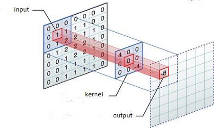
Figure 3.4: The principle of work convolve operation

For applying CNN’s in ranking models proposed in chapters 4 - 5 Caser[Tang and Wang, 2018a] as the baseline presented below (figure 3.5):

Figure 3.5: The network architecture of Caser

The main idea of the model comes from the image recognition field, considering embedding matrix for items as the image and passing the horizontal and vertical convolution filters for searching the local features. As the input the model takes $L$ clicked items for each user $u$ we and their next $T$ ( $T$ is the parameter) items as the targets. To make the recommendations for a user $u$ at time step $t$ using trained Caser, latent user embedding and matrix of trained embeddings for the user’s last $L$ interactions are taken as the input to predict $N$ next items.
•

Recurrent Neural Networks (RNN)

Inside the RNN the basic recurrent cell is located. The model takes input data and pass it through RNN, which has a hidden internal state. This state is updated each time when new data is received in the RNN. Often the task requires that RNN generates some output at each time interval, therefore, after reading the input data and updating the hidden state, the RNN will create the output data.

Figure 3.6: The principle of RNN work. The information is spread from the input to the output with some recursion on the connections between the nodes.

So, what is going on in the green part of the figure 3.6? Inside the green box, the recurrence relation is calculated:

$h_{t}=f_{W}(h_{t-1},x_{t})$ (3.4)

To find the new state $h_{t}$ , the previous hidden state $h_{t-1}$ and the current input $x_{t}$ are taken. When the next input data come to the model, the received hidden state $h_{t}$ is passed through the same function $f_{W}$ , and the whole process is repeated. If there are sufficiently long input sequences, the network could face with the problem of forgetting the information about remote input objects. But in some cases, there is a necessity for the network to "remember" information about the objects located at the beginning of the sequence. To solve this problem, the modifications of RNN, such as GRU and LSTM were proposed.

The authors of the GRU4Rec [Hidasi and Karatzoglou, 2018] adapt the idea of using recurrent neural networks in recommender systems. The basical structure of architecture presented in the figure 3.7, where the main part is a stack of GRU’s.

Figure 3.7: GRU4Recarchitecture

Because of the different session size for each user and the concept of strong time dependency between the interactions inside the session, classical sliding window over the sentences for building mini-batches seems not relevant for recommender systems. That is why authors suggest the strategy from the figure 3.8. First mini-batch is represented by the first event for the first $X$ sessions from the full set of time-ordered sessions. For the second mini-batch the second events are used and so on. When any of the session ends, the next available session is taken.

Figure 3.8: Mini batches for GRU4Rec
•

Graph Neural Networks (GNN)

The idea lying behind Graph Neural Networks (GNN) is to learn a mapping that represents nodes or entire (sub)graphs as points in a low-dimensional vector space. The goal is to optimize this mapping so that the geometric relations in this studied space display the structure of the original graph.

Figure 3.9: LightGCNarchitecture

The normalized sum of neighbor embeddings of LightGCN is taken towards next layer. Proposed by [He et al., 2020] LightGCN for recommendations consists of the graph convolution with the discarded feature transformation and nonlinear activation operations (see figure 3.9). In layer combination part, the final embedding of the node is constructed as the weighted sum of its embeddings on all layers. These models have demonstrated their ability to handle complicated contextual information, such as item summaries generated by extrative summarization approaches [Amini and Usunier, 2007].
•

Transformers

The architecture of Transformers also was designed to process sequences as RNN’s. But unlike RNN’s, transformers do not require processing sequences consecutively. For example, if the input data is text, then the transformer does not need to process the end of the text after processing its beginning. Due to this, transformers are parallelized more easily than RNN’s and can be trained faster

Figure 3.10: The transformer architecture

The main distinctive feature of transformers is in calculating attention, that consists in transforming the embedding vector into three vectors: query, key and value vectors. These vectors are created by multiplying embedding into three matrices that are trained during the training process. As a result, $z$ vector is calculated (see figure 3.10) and then it is transmitted further through forward path of the neural network.

Figure 3.11: SASRectraining structure

In figure 3.11 training process for adapted transformer SASRec proposed by [Kang and McAuley, 2018] is presented. At each time step, the model considers all previous items, and apply attention mechanism to focus on the items relevant to the next action.

3.3 Evaluation metrics

In order to choose the best model from the whole variety of algorithms and approaches, it is necessary to be able to assess their quality quantitatively. In this section, we will present the most common ranking metrics used to evaluate recommender systems.

Consider $N$ users $U=\{u_{i}\}_{i=1}^{N}$ and $M$ items $E=\{e_{j}\}_{j=1}^{K}$ . The result of the ranking algorithm is the mapping, which assigns to each item $e\in E$ the weight $r(e)$ , which characterizes the degree of relevance of this item to the particular user $u\in U$ (the greater the weight, the more relevant the object). That is why the set of weights determines the permutation $\pi$ on the set of items based on their sorting in descending order.

To estimate the quality of the ranking, it is necessary to have some ground true with which the results of the algorithm can be compared. Suggest $r^{true}\in[0,1]$ is the reference relevance characterizes the real relevance of items for a given user ( $r^{true}=1$ item is ideal, $r^{true}=0$ - completely irrelevant), $\pi^{true}$ is the corresponding permutation of $r^{true}(e)$ .

It is worth noting that when $r^{true}$ takes only extreme values: 0 and 1, the permutation $\pi^{true}$ is usually not considered and only the set of relevant items for which $r^{true}=1$ is taken into account. So, the purpose of the metric is to determine how well the relevance obtained by the algorithm and the corresponding permutation $\pi$ to the true relevance values $r^{true}$ . In the next subsections the main metrics would be considered.

3.3.1 Mean Average Precision

Mean average precision at K ( $\text{MAP}@K$ ) is one of the most frequently used ranking metrics. Precision measures are used in binary problem, where relevance accepted two values: 0 and 1.

\text{MAP}@K=\frac{1}{N}\sum_{u=1}^{N}\text{AP}@K.

Here the Average Precision at rank $K$ , AP $@K$ , is defined as :

\text{AP}@K=\frac{1}{K}\sum_{k=1}^{K}r_{k}Pr(k),

where, $Pr(k)$ is the precision at rank $k$ of the relevant items and $r_{k}=1$ if the item at rank $k$ is preferred or clicked, and $0$ otherwise.

The idea of $\text{MAP}@K$ is to calculate $\text{AP}@K$ for each user and then take the average. The idea is quite reasonable, assuming that all users are equally important.

3.3.2 Normalized Discounted Cumulative Gain

If the users are not equally important, simple averaging is not enough to express the quality of ranking. In this case, another popular metric $\text{NDCG}@K$ could be applied. To compute $\text{NDCG}@K$ , the term called $\text{DCG}@K$ is calculated taking into account the order of the items in the list by multiplying the relevance of the item by a weight equal to the inverse logarithm of the position number.

\text{DCG}@K=\sum_{k=1}^{K}\frac{2^{r_{k}}-1}{\log_{2}(1+k)}.

In contrast to $\text{MAP}@K$ , $r_{k}$ here can also be used in the case of non-binary values of the reference relevance. The use of the logarithm as a discount function can be explained by the following intuitive considerations: the positions at the beginning of the ranking differ much more than the positions at the end of it. It means that for a user it is more important to have accurate ranking at the first positions, like 1 to 10, and almost not important how correctly items will be distributed between 50 and 60 positions. Normalized version of $\text{DCG}@K$ is called $\text{NDCG}@K$ and computed below:

\text{NDCG}@K=\frac{1}{N}\sum_{u=1}^{N}\frac{\text{DCG}@K}{\text{IDCG}@K},

where $\text{IDCG}@K$ is $\text{DCG}@K$ with an ideal ordering equals to $\sum_{k=1}^{K}\frac{1}{\log_{2}(1+k)}$ .

3.3.3 Mean reciprocal rank

Another popular metric $\text{MRR}@K$ define at which position of ranking customer find the first useful recommendation.

\text{MRR}@K=\frac{1}{N}\sum_{u=1}^{N}\text{RR}@K,

$\text{RR}@K$ the value equal to the inverse rank of the first correctly predicted item:

\text{RR}@K=\frac{1}{\text{min}\{k\in{1,..,K}:r_{k}=1\}}.

3.3.4 Rank Correlation based metrics

The rank correlation coefficient takes into account not the values of element’s relevances , but only their rank. Below the two most common rank correlation coefficients, the Spearman and Kendall, are presented.

•

Kendall correlation coefficient:

Consider $\{(x_{1},y_{1}),...,(x_{k},y_{k})\}$ be a set of observations of the joint random variables $X$ and $Y$ . Based on the calculation of concordant (and discordant) pairs — pairs of elements to which the permutations have assigned the same (different) order.

$\tau=\frac{|\text{concordant pairs}|-|\text{discordant pairs}|}{K(K-1)/2},$

where concordant pairs are satisfy the condition: both $x_{i}>x_{j}$ and $y_{i}>y_{j}$ hold or both $x_{i}<x_{j}$ and $y_{i}<y_{j}$ hold; otherwise the pairs are discordant.
•

Spearman correlation coefficient:

The Spearman correlation coefficient is defined as the Pearson correlation coefficient between the rank variables.

$r_{S}=\rho(\pi,\pi^{true})=\frac{cov(\pi,\pi^{true})}{\sigma_{\pi},\sigma_{\pi^{true}}},$

$\rho$ denotes the usual Pearson correlation coefficient, but applied to the rank variables.

The quality metrics defined by rank correlation coefficient do not take into account the position of elements and the correlation is calculated for all elements simultaneously, not just for the top-K elements with the highest rank. Therefore, in practice these metrics are applied extremely rarely.

3.4 Conclusion

In this chapter we provided an overview of work on Recommender Systems (RS) that provide personalized recommendations to users by adapting to their taste. The study of RS has become an active area of research these past years, especially since the Netflix Prize [Bennett and Lanning, 2007]. One characteristic of online recommendation is the huge unbalance between the available number of products and those shown to the users. Another aspect is the existence of bots that interact with the system by providing too many feedback over some targeted items; or many users that do not interact with the system over the items that are shown to them. In this context, the main challenges concern the design of a scalable and an efficient online RS in the presence of noise and unbalanced data. These challenges have evolved in time with the continuous development of data collections released for competitions or issued from e-commerce⁴⁴ 4 https://www.kaggle.com/c/outbrain-click-prediction. New approaches for RS now primarily consider implicit feedback, mostly in the form of clicks, that are easier to collect than explicit feedback which is in the form of scores. Implicit feedback is more challenging to deal with as they do not depict the preference of a user over items, i.e., (no)click does not necessarily mean (dis)like [Hu et al., 2008]. For this case, most of the developed approaches are based on the Learning-to-rank paradigm and focus on how to leverage the click information over the unclick one without considering the sequence of users’ interactions.

Part II

Contribution

Chapter 4 Sequential Learning over Implicit Feedback for Robust Large-Scale Recommender Systems

4.1 Introduction

In this chapter, we propose our first contribution which is a new SequentiAl RecOmmender System for implicit feedback (called SAROS), that updates the model parameters user per user over blocks of items constituted by a sequence of unclicked items followed by a clicked one. The parameter updates are discarded for users who interact very little or a lot with the system. For other users, the update is done by minimizing the average ranking loss of the current model that scores the clicked item below the unclicked ones in a corresponding block. Recently, many other approaches that model the sequences of users feedback have been proposed, but they all suffer from a lack of theoretical analysis formalizing the overall learning strategy. In this work, we analyze the convergence property of the proposed approach and show that in the case where the global ranking loss estimated over all users and items is convex; then the minimizer found by the proposed sequential approach converges to the minimizer of the global ranking loss. Experimental results conducted on five large publicly available datasets show that our approach is highly competitive compared to the state-of-the-art models and, it is significantly faster than both the batch and the online versions of the algorithm. The results of this chapter were presented at the European Conference in Machine Learning & Principles ans Practices in Knowledge Discovery (ECML-PKDD) in 2019 [4] and Conférence sur l’Apprentissage Automatique (CAp) in 2021 [3].

The rest of this chapter is organized as follows. Section 4.2 relates our work to previously proposed approaches. Section 4.3 introduces the general ranking learning problem that we address. Then, in Section 4.4, we present the SAROS algorithm and provide an analysis of its convergence. Section 4.5 presents the experimental results that support this approach. Finally, in Section 4.6, we discuss the outcomes of this study and give some pointers to further research.

4.2 Sequential learning for recommender systems

Many new approaches tackle the sequential learning problem for RS by taking into account the temporal aspect of interactions directly in the design of a dedicated model and are mainly based on Markov Models (MM), Reinforcement Learning (RL) and Recurrent Neural Networks (RNN) [Donkers et al., 2017]. Recommender systems based on Markov Models, consider the sequential interaction of users as a stochastic process over discrete random variables related to predefined user behavior. These approaches suffer from some limitations mainly due to the sparsity of the data leading to a poor estimation of the transition matrix [Shani et al., 2005]. Various strategies have been proposed to leverage the impact of sparse data, for example by considering only the last frequent sequences of items and using finite mixture models [Shani et al., 2005], or by combining similarity-based methods with high-order Markov Chains [Ruining and Julian, 2016]. Although it has been shown that in some cases the proposed approaches can capture the temporal aspect of user interactions but these models suffer from high complexity and generally they do not pass the scale. Some other methods consider RS as a Markov decision process (MDP) problem and solve it using reinforcement learning (RL) [Moling et al., 2012, Tavakol and Brefeld, 2014]. The size of discrete actions bringing the RL solver to a larger class of problems is also a bottleneck for these approaches. Very recently Recurrent neural networks such as GRU or LSTM, have been proposed for personalized recommendations [Hidasi and Karatzoglou, 2018, Tang and Wang, 2018a, Kang and McAuley, 2018], where the input of the network is generally the current state of the session, and the output is the predicted preference over items (probabilities for each item to be clicked next).

Our proposed strategy differs from other sequential based approaches in the way that the model parameters are updated, at each time a block of unclicked items followed by a clicked one is constituted; and by controlling the number of blocks per user interaction. If for a given user, this number is below or above two predefined thresholds found over the distribution of the number of blocks, parameter updates for that particular user are discarded. Ultimately, we provide a proof of convergence of the proposed approach.

4.3 Framework and Problem Setting

Throughout, we use the following notation. For any positive integer $n$ , $[n]$ denotes the set $[n]\doteq\{1,\ldots,n\}$ . We suppose that $\mathcal{I}\doteq[M]$ and $\mathcal{U}\doteq[N]$ are two sets of indexes defined over items and users. Further, we assume that each pair constituted by a user $u$ and an item $i$ is identically and independently distributed according to a fixed yet unknown distribution ${\cal D}_{\cal U,\cal I}$ .

At the end of his or her session, a user $u\in\mathcal{U}$ has reviewed a subset of items $\mathcal{I}_{u}\subseteq\mathcal{I}$ that can be decomposed into two sets: the set of preferred and non-preferred items denoted by $\mathcal{I}^{+}_{u}$ and $\mathcal{I}^{-}_{u}$ , respectively. Hence, for each pair of items $(i,i^{\prime})\in\mathcal{I}^{+}_{u}\times\mathcal{I}^{-}_{u}$ , the user $u$ prefers item $i$ over item $i^{\prime}$ ; symbolized by the relation $i\!\begin{array}[]{c}{\succ}\\ \mbox{{\tiny{\it u}}}\end{array}\!i^{\prime}$ . From this preference relation a desired output $y_{u,i,i^{\prime}}\in\{-1,+1\}$ is defined over the pairs $(u,i)\in\mathcal{U}\times\mathcal{I}$ and $(u,i^{\prime})\in\mathcal{U}\times\mathcal{I}$ , such that $y_{u,i,i^{\prime}}=+1$ if and only if $i\!\begin{array}[]{c}{\succ}\\ \mbox{{\tiny{\it u}}}\end{array}\!i^{\prime}$ . We suppose that the indexes of users as well as those of items in the set $\mathcal{I}_{u}$ , shown to the active user $u\in\mathcal{U}$ , are ordered by time.

Finally, for each user $u$ , parameter updates are performed over blocks of consecutive items where a block $\mathcal{B}_{u}^{t}=\text{N}_{u}^{t}\sqcup\Pi_{u}^{t}$ , corresponds to a time-ordered sequence (w.r.t. the time when the interaction is done) of no-preferred items, $\text{N}_{u}^{t}$ , and at least one preferred one, $\Pi_{u}^{t}$ . Hence, $\mathcal{I}^{+}_{u}=\bigcup_{t}\Pi_{u}^{t}$ and $\mathcal{I}^{-}_{u}=\bigcup_{t}\text{N}_{u}^{t};\forall u\in\mathcal{U}$ . Notations are summarized in Table 4.1.

$\mathcal{I}=[M]$	The set of item indexes
$\mathcal{U}=[N]$	The set of user indexes
${\cal D}$	joint distribution over users and items
${\cal D}_{u}$	conditional distribution of items for a fixed user $u$
$\text{N}_{u}^{t}$	Negative items in block $t$ for user $u$
$\Pi_{u}^{t}$	Positive items in block $t$ for user $u$
$\mathcal{B}_{u}^{t}=\text{N}_{u}^{t}\sqcup\Pi_{u}^{t}$	Negative and positive items in block $t$ for user $u$
$\mathcal{I}^{+}_{u}$	The set of all positive items for user $u$
$\mathcal{I}^{-}_{u}$	The set of all negative items for user $u$
$\ell_{u,i,i^{\prime}}(\omega)$	Instantaneous loss for user $u$ and a pair of items $(i,i^{\prime})$
$\hat{\mathcal{L}}_{u}(\omega)$	Empirical ranking loss with respect to user $u$
	$\hat{\mathcal{L}}_{u}(\omega)=\frac{1}{\|\mathcal{I}^{+}_{u}\|\|\mathcal{I}^{-}_{u}\|}\!\sum_{i\in\mathcal{I}^{+}_{u}}\!\sum_{i^{\prime}\in\mathcal{I}^{-}_{u}}\!\ell_{u,i,i^{\prime}}(\omega)$
${\hat{\mathcal{L}}}_{\mathcal{B}^{t}_{u}}(\omega)$	Empirical ranking loss with respect to a block of items
	${\hat{\mathcal{L}}}_{\mathcal{B}^{t}_{u}}(\omega)=\frac{1}{\|\Pi_{u}^{t}\|\|\text{N}_{u}^{t}\|}\sum_{i\in\Pi_{u}^{t}}\sum_{i^{\prime}\in\text{N}_{u}^{t}}\ell_{u,i,i^{\prime}}(\omega)$
${\mathcal{L}}(\omega)$	Expected ranking loss ${\mathcal{L}}(\omega)=\mathbb{E}_{{\cal D}_{u}}\hat{\mathcal{L}}_{u}(\omega)$

Table 4.1: Notation for the proposed SAROS algorithm and its variants.

4.4 Proposed Approach

Our objective here is to minimize an expected error penalizing the misordering of all pairs of interacted items $i$ and $i^{\prime}$ for a user $u$ . Commonly, this objective is given under the Empirical Risk Minimization (ERM) principle, by minimizing the empirical ranking loss estimated over the items and the final set of users who interacted with the system :

\hat{\mathcal{L}}_{u}(\bm{\omega})\!=\!\frac{1}{|\mathcal{I}^{+}_{u}||\mathcal{I}^{-}_{u}|}\!\sum_{i\in\mathcal{I}^{+}_{u}}\!\sum_{i^{\prime}\in\mathcal{I}^{-}_{u}}\!\ell_{u,i,i^{\prime}}(\bm{\omega}),

(4.1)

and $\mathcal{L}(\bm{\omega})={\mathbb{E}}_{u}\left[\hat{\cal L}_{u}(\bm{\omega})\right]$ , where ${\mathbb{E}}_{u}$ is the expectation with respect to users chosen randomly according to the uniform distribution, and $\hat{\mathcal{L}}_{u}(\bm{\omega})$ is the pairwise ranking loss with respect to user $u$ ’s interactions. As in other studies, we represent each user $u$ and each item $i$ respectively by vectors $\mathbf{U}_{u}\in\mathbb{R}^{k}$ and $\mathbf{V}_{i}\in\mathbb{R}^{k}$ in the same latent space of dimension $k$ [Koren et al., 2009]. The set of weights to be found $\bm{\omega}=(\mathbf{U},\mathbf{V})$ , are then matrices formed by the vector representations of users $\mathbf{U}=(\mathbf{U}_{u})_{u\in[N]}\in\mathbb{R}^{N\times k}$ and items $\mathbf{V}=(\mathbf{V}_{i})_{i\in[M]}\in\mathbb{R}^{M\times k}$ . The minimization of the ranking loss above in the batch mode with the goal of finding user and item embeddings, such that the dot product between these representations in the latent space reflects the best the preference of users over items, is a common approach. Other strategies have been proposed for the minimization of the empirical loss (4.1), among which the most popular one is perhaps the Bayesian Personalized Ranking (BPR) model [Rendle et al., 2009]. In this approach, the instantaneous loss, $\ell_{u,i,i^{\prime}}$ , is the surrogate regularized logistic loss for some hyperparameter $\mu\geq 0$ :

\hskip-2.84526pt\ell_{u,i,i^{\prime}}(\bm{\omega})=\log\left(1+e^{-y_{i,u,i^{\prime}}\mathbf{U}_{u}^{\top}(\mathbf{V}_{i}-\mathbf{V}_{i^{\prime}})}\right)+\mu(\|\mathbf{U}_{u}\|_{2}^{2}+\|\mathbf{V}_{i}\|_{2}^{2}+\|\mathbf{V}_{i^{\prime}}\|_{2}^{2})

(4.2)

The BPR algorithm proceeds by first randomly choosing a user $u$ , and then repeatedly selecting two pairs $(i,i^{\prime})\in\mathcal{I}_{u}\times\mathcal{I}_{u}$ .

In the case where one of the chosen items is preferred over the other one (i.e. $y_{u,i,i^{\prime}}\in\{-1,+1\}$ ), the algorithm then updates the weights using the stochastic gradient descent method over the instantaneous loss (4.2). In this case, the expected number of rejected pairs is proportional to $O(|\mathcal{I}_{u}|^{2})$ [Sculley, 2009] which may be time-consuming in general. Another drawback is that user preference over items depend mostly on the context where these items are shown to the user. A user may prefer (or not) two items independently one from another, but within a given set of shown items, he or she may completely have a different preference over these items. By sampling items over the whole set of shown items, this effect of local preference is unclear.

4.4.1 Algorithm SAROS

Another particularity of online recommendation which is not explicitly taken into account by existing approaches is the bot attacks in the form of excessive clicks over some target items. They are made to force the RS to adapt its recommendations toward these target items, or a very few interactions which in both cases introduce biased data for the learning of an efficient RS. In order to tackle these points, our approach updates the parameters whenever the number of constituted blocks per user is lower and upper-bounded (Figure 4.1).

In this case, at each time a block $\mathcal{B}_{u}^{t}=\text{N}_{u}^{t}\sqcup\Pi_{u}^{t}$ is formed; weights are updated by miniminzing the ranking loss corresponding to this block :

{\hat{\cal L}}_{\mathcal{B}_{u}^{t}}(\bm{\omega}_{u}^{t})=\frac{1}{|\Pi_{u}^{t}||\text{N}_{u}^{t}|}\sum_{i\in\Pi_{u}^{t}}\sum_{i^{\prime}\in\text{N}_{u}^{t}}\ell_{u,i,i^{\prime}}({\bm{\omega}}_{u}^{t}).

(4.3)

The pseudo-code of SAROS is shown in the following. Starting from initial weights $\bm{\omega}_{1}^{0}$ chosen randomly for the first user. For each current user $u$ , having been shown $I_{u}$ items, the sequential update rule consists in updating the weights, block by block where after $t$ updates; where the $(t+1)^{th}$ update over the current block $\mathcal{B}_{u}^{t}=\text{N}_{u}^{t}\sqcup\Pi_{u}^{t}$ corresponds to one gradient descent step over the ranking loss estimated on these sets and which with the current weights $\bm{\omega}_{u}^{t}$ writes,

\bm{\omega}_{u}^{t+1}\leftarrow\bm{\omega}_{u}^{t}-\eta\nabla{\hat{\cal L}}_{\mathcal{B}_{u}^{t}}(\bm{\omega}_{u}^{t})

(4.4)

Algorithm 1 *

Algorithm SAROS: SequentiAl RecOmmender System

Input: A time-ordered sequence (user and items)

\{(u,(i_{1},\dots,i_{|I_{u}|})\}_{u=1}^{N}

drawn i.i.d. from

{\cal D}_{{\cal U},{\cal I}}

Input: maximal

B

and minimal

b

number of blocks allowed per user

u

Input: number of epochs

E

Input: initial parameters

\omega_{1}^{0}

, and (possibly non-convex) surrogate loss function

\ell(\omega)

for

e\in E

for

u\in\mathcal{U}

Let

\text{N}_{u}^{t}=\varnothing,\,\Pi_{u}^{t}=\varnothing

be the sets of positive and negative items, counter

t=0

for

i_{k}\in\mathcal{I}_{u}

\triangleright

Consider all items displayed to user

u

while

t\leq B

u

provides a negative feedback on item

i_{k}

then

\text{N}_{u}^{t}\leftarrow\text{N}_{u}^{t}\cup\{i_{k}\}

else

\Pi_{u}^{t}\leftarrow\Pi_{u}^{t}\cup\{i_{k}\}

end if

\text{N}_{u}^{t}\neq\varnothing

and

\Pi_{u}^{t}\neq\varnothing

and

t\leq B

then

\bm{\omega}_{u}^{t+1}\leftarrow\bm{\omega}_{u}^{t}-\frac{\eta}{|{\text{N}_{u}^{t}}||\Pi_{u}^{t}|}\displaystyle{\sum_{i\in\Pi_{u}^{t}}\sum_{i^{\prime}\in\text{N}_{u}^{t}}}\nabla\ell_{u,i,i^{\prime}}(\bm{\omega}_{u}^{t})

t=t+1,\text{N}_{u}^{t}=\varnothing

\Pi_{u}^{t}=\varnothing

end if

end while

end for

t\geq b

then

{\omega}_{u+1}^{0}={\omega}_{u}^{t}

else

{\omega}_{u+1}^{0}={\omega}_{u}^{0}

end if

end for

Return:

{\bar{\omega}}_{N}=\sum_{u\in\mathcal{U}}\omega_{u}^{0}

To prevent from a very few interactions or from bot attacks, two thresholds $b$ and $B$ are fixed over the parameter updates. For a new user $u+1$ , the parameters are initialized as the last updated weights from the previous user’s interactions in the case where the corresponding number of updates $t$ was in the interval $[b,B]$ ; i.e. $\omega^{0}_{u+1}=\omega^{t}_{u}$ . On the contrary case, they are set to the same previous initial parameters; i.e., $\omega^{0}_{u+1}=\omega^{0}_{u}$ .

4.4.2 Convergence analysis

We provide proofs of convergence for the SAROS algorithm under the typical hypothesis that the system is not instantaneously affected by the sequential learning of the weights. This hypothesis stipulates that the generation of items shown to users is independently and identically distributed with respect to some stationary in time underlying distribution ${\cal D}_{\cal I}$ , and constitutes the main hypothesis of almost all the existing studies. Furthermore, we make the following technical assumption.

Assumption 1

Let the loss functions $\ell_{u,i,i^{\prime}}(\omega)$ and ${\cal L}(\omega)$ , $\omega\in\mathbb{R}^{d}$ be such that for some absolute constants $\gamma\geq\beta>0$ and $\sigma>0$ :

1.

$\ell_{u,i,i^{\prime}}(\omega)$ is non-negative for any user $u$ and a pair of items $(i,i^{\prime})$ ;
2.

$\ell_{u,i,i^{\prime}}(\omega)$ is twice continuously differentiable, with a continuous Lipschitz gradient for both instantaneous loss and the ranking loss (Chapter 2 definition 1). That is for any user $u$ and a pair of items $(i,i^{\prime})$ we have $\|\nabla\ell_{u,i,i^{\prime}}(\omega)-\nabla\ell_{u,i,i^{\prime}}(\omega^{\prime})\|_{2}\leq\gamma\|\omega-\omega^{\prime}\|_{2},$ as well as $\|\nabla{\cal L}(\omega)-\nabla{\cal L}(\omega^{\prime})\|_{2}\leq\beta\|\omega-\omega^{\prime}\|_{2},$ .
3.

Variance of the empirical loss is bounded $\mathbb{E}_{\cal D}\left\|\nabla\hat{\cal L}_{u}(\omega)-\nabla{\cal L}(\omega)\right\|_{2}^{2}\leq\sigma^{2}.$

Moreover, there exist some positive lower and upper bounds $b$ and $B$ , such that the number of updates for any $u$ is within the interval $[b,B]$ almost surely.

Our main result in this chapter is the following theorem which provides a bound over the deviation of the ranking loss with respect to the sequence of weights found by the SAROS algorithm and its minimum in the case where the latter is convex.

Theorem 4 ([4])

Let $\ell_{u,i,i^{\prime}}(\omega)$ and ${\cal L}(\omega)$ satisfy Assumption 1. Then for any constant step size $\eta$ , verifying $0<\eta\leq\min(\frac{1}{\beta B},1/\sqrt{UB(\sigma^{2}+3\gamma^{2}/b)})$ , and any set of users $\mathcal{U}\doteq[U]$ ; algorithm SAROS iteratively generates a sequence $\{\omega_{u}^{0}\}_{u\in\mathcal{U}}$ such that

\displaystyle\frac{1}{\beta}\mathbb{E}\|\nabla{\cal L}({\omega}_{u}^{0})\|_{2}^{2}\leq\frac{\beta B\Delta_{\cal L}^{2}}{u}+2\Delta_{\cal L}\sqrt{\frac{B\sigma^{2}+3B\gamma^{2}/b}{u}},

where $\Delta_{\cal L}^{2}={\frac{2}{\beta}({\cal L}(\omega_{0})-{\cal L}(\omega^{*}))}$ , and the expectation is taken with respect to users chosen randomly according to the uniform distribution $p_{u}=\frac{1}{N}$ .

Furthermore, if the ranking loss ${\cal L}(\omega)$ is convex, then for the sequence $\{\omega_{u}^{0}\}_{u\in\mathcal{U}}$ generated by algorithm SAROS and $\bar{\omega}_{u}=\sum_{j\leq u}\omega_{j}^{0}$ we have

\displaystyle{\cal L}({\bar{\omega}}_{u})-{\cal L}({\omega_{*}})\leq\frac{\beta B\Delta_{\omega}^{2}}{u}+2\Delta_{\omega}\sqrt{\frac{B\sigma^{2}+3B\gamma^{2}/b}{u}},

where $\Delta_{\omega}=\|\omega_{0}-\omega_{*}\|_{2}^{2}$ , and $\omega_{*}=\mathop{\argmin}_{\omega}{\cal L}({\omega})$ .

Proof. Sketch. Expectation of the empirical loss taken over a random block ${\cal B}_{u}^{t}$ for a user $u$ , equals to the expected loss for this user. Then by the law of total expectation one has $\mathbb{E}_{{\cal D}_{u}}\left[k^{-1}\sum_{l=1}^{k}\nabla{\hat{\cal L}}_{\mathcal{B}^{l}_{u}}(\bm{\omega})\right]=\nabla\hat{\cal L}_{u}(\omega)$ , where ${\cal D}_{u}$ is the conditional distribution of items for a fixed user $u$ . The variance of the gradient estimation over $k$ blocks is bounded by $3\gamma^{2}/k$ , as for any block after the next to ${\cal B}_{u}^{t}$ and before the previous to ${\cal B}_{u}^{t}$ are conditionally independent for any fixed ${\cal B}_{u}^{t}$ .

Let $g_{u}^{t}$ be a gradient of the loss function taken for user $u$ over block ${\cal B}^{t}_{u}$ :

g_{u}^{t}=\frac{1}{|N_{u}^{t}||\Pi_{u}^{t}|}\sum_{i\in N_{u}^{t},i^{\prime}\in\Pi_{u}^{t}}\nabla\ell_{u,i,i^{\prime}}(\omega_{u}^{t-1}),

According to the notation of Algorithm SAROS let $\delta_{u}^{t}=g_{u}^{t}-\nabla{\cal L}(\omega_{u}^{0})$ and $\omega_{u}^{t+1}=\omega_{u}^{t}-\eta g_{u}^{t}$ , $\omega_{u+1}^{0}=\omega_{u}^{|{\cal B}_{u}|}$ , and $\omega_{u+1}^{0}-\omega_{u}^{0}=\eta\sum_{t\in{\cal B}_{u}}g_{u}^{t}$ , where ${\cal B}_{u}$ is the set of all interacted blocks corresponding to user $u$ . Using the smoothness of the loss function implied by Assumption 1, it comes :

	$\displaystyle{\cal L}(\omega_{u+1}^{0})$	$\displaystyle={\cal L}(\omega_{u}^{0})-\left(\hat{\eta}_{u}-\frac{\beta}{2}{\hat{\eta}}^{2}_{u}\right)\\|\nabla{\cal L}(\omega_{u}^{0})\\|_{2}^{2}$
		$\displaystyle-(\hat{\eta}_{u}-\beta{\hat{\eta}}^{2}_{u})\sum_{t\in{\cal B}_{u}}\left\langle\nabla{\cal L}(\omega_{u}^{0}),\frac{\delta_{u}^{t}}{\|{\cal B}_{u}\|}\right\rangle+\frac{\beta}{2}{\hat{\eta}}^{2}_{u}\sum_{t\in{\cal B}_{u}}\left\\|\frac{\delta_{u}^{t}}{\|{\cal B}_{u}\|}\right\\|_{2}^{2}$		(4.5)

where $\hat{\eta}_{u}=|{\cal B}_{u}|\eta$ . Then by re-arranging and summing up, we get

	$\displaystyle\sum_{u=1}^{N}$	$\displaystyle\left(\hat{\eta}_{u}-\frac{\beta}{2}{\hat{\eta}}^{2}_{u}\right)\\|\nabla{\cal L}(\omega_{u})\\|_{2}^{2}\leq{\cal L}(\bar{\omega}_{u})-{\cal L}(\omega^{*})$
		$\displaystyle-\sum_{u=1}^{N}(\hat{\eta}_{u}-\beta\hat{\eta}^{2}_{u})\left\langle\nabla{\cal L}(\omega_{u}),\sum_{t\in{\cal B}_{u}}\frac{\delta_{u}^{t}}{\|{\cal B}_{u}\|}\right\rangle+\frac{\beta}{2}\sum_{u=1}^{N}\hat{\eta}_{u}^{2}\left\\|\sum_{t\in{\cal B}_{u}}\frac{\delta_{u}^{t}}{\|{\cal B}_{u}\|}\right\\|_{2}^{2}$

As the stochastic gradient taken with respect to a block of items gives an unbiased estimate of the gradient, thus

\displaystyle\mathbb{E}_{{\cal D}_{u}}\biggl[\biggl\langle\nabla{\cal L}(\omega_{u}),\sum_{t\in{\cal B}_{u}}\frac{\delta_{u}^{t}}{|{\cal B}_{u}|}\biggr\rangle\bigg|\xi_{u}\biggr]=0,

(4.6)

where $\xi_{u}$ is a set of users preceding $u$ . As in the conditions of the theorem $b\leq|{\cal B}_{u}|$ almost surely, by the law of total variation, $\Var\psi=\mathbb{E}[\Var(\psi|\eta)]+\Var[\mathbb{E}[\psi|\eta]]$ :

\displaystyle\mathbb{E}_{{\cal D}_{u}}\,\left\|\sum_{t\in{\cal B}_{u}}\frac{\delta_{u}^{t}}{|{\cal B}_{u}|}\right\|_{2}^{2}\leq\sigma^{2}+\frac{3\gamma^{2}}{b}

(4.7)

where the first term on the right-hand side of Eq. (4.7) comes from Assumption 1, and the second term is due to the variance estimate. Condition $\beta\eta B\leq 1$ implies $\hat{\eta}_{u}-{\beta}{\hat{\eta}}^{2}_{u}/2\geq\hat{\eta}_{u}/2$ , thus

\displaystyle\frac{1}{\beta}\mathbb{E}_{\cal D}\,\|\nabla{\cal L}(\omega)\|_{2}^{2}\leq\frac{1}{\sum_{u=1}^{N}\hat{\eta}_{u}}\left[\frac{2({\cal L}(\omega_{0})-{\cal L}(\omega_{*}))}{\beta}+\left(\sigma^{2}+3\frac{\gamma^{2}}{b}\right)\sum_{u=1}^{N}\hat{\eta}^{2}_{u}\right]

The rest of the proof of the theorem comes along the same lines according to the randomized stochastic gradient descent analysis [Ghadimi and Lan, 2013]. $\square$

The full proof is provided in the Supplementary. This result implies that the loss over a sequence of weights $(\omega_{u}^{0})_{u\in\mathcal{U}}$ generated by the algorithm converges to the true minimizer of the ranking loss ${\cal L}(\omega)$ with a rate proportional to $O({1}/{\sqrt{u}})$ . The stochastic gradient descent strategy implemented in the Bayesian Personalized Ranking model (BPR) [Rendle et al., 2009] also converges to the minimizer of the ranking loss ${\cal L}(\omega)$ with the same rate. However, the main difference between BPR and SAROS is their computation time. As stated previously, the expected number of rejected random pairs sampled by algorithm BPR before making one update is $O(|\mathcal{I}_{u}|^{2})$ while with SAROS, blocks are created sequentially as and when users interact with the system. For each user $u$ , weights are updated whenever a block is created, with the overall complexity of $O(\max_{t}(|\Pi_{u}^{t}|\times|\text{N}_{u}^{t}|))$ , with $\max_{t}(|\Pi_{u}^{t}|\times|\text{N}_{u}^{t}|)\ll|\mathcal{I}_{u}|^{2}$ .

4.5 Experimental Setup and Results

In this section, we provide an empirical evaluation of our optimization strategy on some popular benchmarks proposed for evaluating RS. All subsequently discussed components were implemented in Python3 using the TensorFlow library ¹¹ 1 https://www.tensorflow.org/. and computed on Skoltech CDISE HPC cluster “Zhores” [Zacharov et al., 2019]. We first proceed with a presentation of the general experimental set-up, including a description of the datasets and the baseline models.

Datasets.

We report results obtained on five publicly available datasets, for the task of personalized Top-N recommendation on the following collections :

•

ML-1M [Harper and Konstan, 2015] and Netflix [Bennett and Lanning, 2007] consist of user-movie ratings, on a scale of one to five, collected from a movie recommendation service and the Netflix company. The latter was released to support the Netflix Prize competition [Bennett and Lanning, 2007]. For both datasets, we consider ratings greater or equal to $4$ as positive feedback, and negative feedback otherwise.
•

We extracted a subset out of the Outbrain dataset from of the Kaggle challenge²² 2 https://www.kaggle.com/c/outbrain-click-prediction that consisted in the recommendation of news content to users based on the 1,597,426 implicit feedback collected from multiple publisher sites in the United States.
•

Kasandr³³ 3 https://archive.ics.uci.edu/ml/datasets/KASANDR dataset [Sidana et al., 2017] contains 15,844,717 interactions of 2,158,859 users in Germany using Kelkoo’s (http://www.kelkoo.fr/) online advertising platform.
•

Pandor⁴⁴ 4 https://archive.ics.uci.edu/ml/datasets/PANDOR is another publicly available dataset for online recommendation [Sidana et al., 2018] provided by Purch (http://www.purch.com/). The dataset records 2,073,379 clicks generated by 177,366 users of one of the Purch’s high-tech website over 9,077 ads they have been shown during one month.

Table 4.2 presents some detailed statistics about each collection. Among these, we report the average number of positive (click, like) feedback and the average number of negative feedback. As we see from the table, Outbrain, Kasandr, and Pandor datasets are the most unbalanced ones in regards to the number of preferred and non-preferred items.

Data	$\|\mathcal{U}\|$	$\|\mathcal{I}\|$	Sparsity	Avg. # of $+$	Avg. # of $-$
ML-1M	6,040	3,706	.9553	95.2767	70.4690
Outbrain	49,615	105,176	.9997	6.1587	26.0377
Pandor	177,366	9,077	.9987	1.3266	10.3632
Netflix	90,137	3,560	.9914	26.1872	20.2765
Kasandr	2,158,859	291,485	.9999	2.4202	51.9384

Table 4.2: Statistics on the # of users and items; as well as the sparsity and the average number of

+

(preferred) and

-

(non-preferred) items on ML-1M, Netflix, Outbrain, Kasandr and Pandor collections after preprocessing.

Dataset	$\|S_{train}\|$	$\|S_{test}\|$	$pos_{train}$	$pos_{test}$
ML-1M	797,758	202,451	58.82	52.39
Outbrain	1,261,373	336,053	17.64	24.73
Pandor	1,579,716	493,663	11.04	12.33
Netflix	3,314,621	873,477	56.27	56.70
RecSys’16	5,048,653	1,281,909	17.07	13.81
Kasandr	12,509,509	3,335,208	3.36	8.56

Table 4.3: Number of interactions used for train and test on each dataset, and the percentage of positive feedback among these interactions.

To construct the training and the test sets, we discarded users who did not interact over the shown items and sorted all interactions according to time-based on the existing time-stamps related to each dataset. Furthermore, we considered $80\%$ of each user’s first interactions (both positive and negative) for training, and the remaining for the test. Table 4.3 presents the size of the training and the test sets as well as the percentage of positive feedback (preferred items) for all collections ordered by increasing training size. The percentage of positive feedback is inversely proportional to the size of the training sets, attaining $3\%$ for the largest, Kasandr collection.

We also analyzed the distributions of the number of blocks and their size for different collections. Figure 4.2 (left) shows boxplots representing the logarithm of the number of blocks through their quartiles for all collections. From these plots, it comes out that the distribution of the number of blocks on Pandor, Netflix and Kasandr are heavy-tailed with more than the half of the users interacting no more than 10 times with the system. Furthermore, we note that on Pandor the average number of blocks is much smaller than on the two other collections; and that on all three collections the maximum numbers of blocks are $10$ times more than the average. These plots suggest that a very small number of users (perhaps bots) have an abnormal interaction with the system generating a huge amount of blocks on these three collections. To have a better understanding, Figure 4.2 (right) depicts the number of blocks concerning their size on Kasandr. The distribution of the number of blocks follows a power law distribution and it is the same for the other collections that we did not report for the sake of space. In all collections, the number of blocks having more than $5$ items drops drastically. As the SAROS does not sample positive and negative items for updating the weights, these updates are performed on blocks of small size, and are made very often.


(a)		(b)

Figure 4.2: (a) Boxplots depicting the logarithm of the number of blocks through their quartiles for all collections. The median (resp. mean) is represented by the band (resp. diamond) inside the box. The ends of the whiskers represent the minimum and the maximum of the values. (b) Distributions of negative feedback over the blocks in the training set on Kasandr.

Compared approaches.

To validate the sequential approach described earlier, we compared the proposed SAROS algorithm⁵⁵ 5 The code is available on https://github.com/SashaBurashnikova/SAROS. with the following methods:

•

MostPop is a non-learning based approach which consists in recommending the same set of popular items to all users.
•

Matrix Factorization (MF) [Koren, 2008], is a factor model which decomposes the matrix of user-item interactions into a set of low dimensional vectors in the same latent space, by minimizing a regularized least square error between the actual value of the scores and the dot product over the user and item representations.
•

BPR [Rendle et al., 2009] corresponds to the model described in the problem statement above, a stochastic gradient-descent algorithm, based on bootstrap sampling of training triplets, and BPR_b the batch version of the model which consists in finding the model parameters $\bm{\omega}=(\mathbf{U},\mathbf{V})$ by minimizing the global ranking loss over all the set of triplets simultaneously (Eq. 4.1).
•

Prod2Vec [Grbovic et al., 2015], learns the representation of items using a Neural Networks based model, called word2vec [Mikolov et al., 2013a], and performs next-items recommendation using the similarity between the representations of items.
•

GRU4Rec $+$ [Hidasi and Karatzoglou, 2018] is an extended version of GRU4Rec [Hidasi et al., 2016a] adopted to different loss functions, that applies recurrent neural network with a GRU architecture for session-based recommendation. The approach considers the session as the sequence of clicks of the user that depends on all the previous ones for learning the model parameters by optimizing a regularized approximation of the relative rank of the relevant item which favors the preferred items to be ranked at the top of the list.
•

Caser [Tang and Wang, 2018a] is a CNN based model that embeds a sequence of interactions into a temporal image and latent spaces and find local characteristics of the temporal image using convolution filters.
•

SASRec [Kang and McAuley, 2018] uses an attention mechanism to capture long-term semantics and then predicts the next item to present based on a user’s action history.

Hyper-parameters of different models and the dimension of the embedded space for the representation of users and items; as well as the regularisation parameter over the norms of the embeddings for BPR, BPR_b, MF, Caser and SAROS approaches were found by cross-validation. We fixed $b$ and $B$ , used in SAROS, to respectively the minimum and the average number of blocks found on the training set of each corresponding collection. With the average number of blocks being greater than the median on all collections, the motivation here is to consider the maximum number of blocks by preserving the model from the bias brought by the too many interactions of the very few number of users. For more details regarding the exact values for the parameters, see the Table 4.4.

Parameter	ML	Outbrain	Pandor	Netflix	Kasandr
$B$	78	5	2	22	5
$b$	1	2	1	1	1
Learning rate	.05	.05	.05	.05	.4

Table 4.4: SAROS parameters values.

Evaluation setting and results.

We begin our comparisons by testing BPR_b, BPR and SAROS approaches over the logistic ranking loss (Eq. 4.2) which is used to train them. Results on the test, after training the models 30 minutes and at convergence are shown in Table 4.5. BPR_b (resp. SAROS) techniques have the worse (resp. best) test loss on all collections, and the difference between their performance is larger for bigger size datasets.

Dataset	Test Loss, Eq. (4.1)
		30 min			At convergence
		BPR_b	BPR	SAROS	BPR_b	BPR	SAROS
ML-1M		0.751	0.678	0.623	0.744	0.645	0.608
Outbrain		0.753	0.650	0.646	0.747	0.638	0.635
Pandor		0.715	0.671	0.658	0.694	0.661	0.651
Netflix		0.713	0.668	0.622	0.694	0.651	0.614
Kasandr		0.663	0.444	0.224	0.631	0.393	0.212

Table 4.5: Comparison between BPR, BPR_b and SAROS approaches in terms on test loss after

30

minutes of training and at convergence.

These results suggest that the local ranking between preferred and no-preferred items present in the blocks of the training set reflects better the preference of users than the ranking of random pairs of items or their global ranking without this contextual information. Furthermore, as in SAROS updates occur after the creation of a block, and that the most of the blocks contain very few items (Figure 4.2 - right), weights are updated more often than in BPR or BPR_b. This is depicted in Figure 4.3 which shows the evolution of the training error over time for BPR_b, BPR and SAROS on all collections. As we can see, the training error decreases in all cases, and theoretically, the three approaches converge to the same minimizer of the ranking loss (Eq. 4.1). However, the speed of convergence is much faster with SAROS.


(a) Outbrain	(b) Pandor

(c) Netflix	(d) Kasandr

Figure 4.3: Evolution of the loss on training sets for both BPR_b, BPR and SAROS as a function of time in minutes for all collections.

We also compare the performance of all the approaches on the basis of the common ranking metrics, which are the Mean Average Precision at rank $K$ (MAP@K) over all users defined as $\texttt{MAP@K}=\frac{1}{N}\sum_{u=1}^{N}\texttt{AP@K}(u)$ , where $\texttt{AP@K}(u)$ is the average precision of preferred items of user $u$ in the top $K$ ranked ones; and the Normalized Discounted Cumulative Gain at rank $K$ (NDCG@K) that computes the ratio of the obtained ranking to the ideal case and allow to consider not only binary relevance as in Mean Average Precision, $\texttt{NDCG@K}=\frac{1}{N}\sum_{u=1}^{N}\frac{\texttt{DCG@K}(u)}{\texttt{IDCG@K}(u)}$ , where $\texttt{DCG@K}(u)=\sum_{i=1}^{K}\frac{2^{rel_{i}}-1}{\log_{2}(1+i)}$ , $rel_{i}$ is the graded relevance of the item at position $i$ ; and $\texttt{IDCG@K}(u)$ is $\texttt{DCG@K}(u)$ with an ideal ordering equals to $\sum_{i=1}^{K}\frac{1}{\log_{2}(1+i)}$ for $rel_{i}\in[0,1]$ [Schutze et al., 2008].

Table 4.6 presents MAP@5 and MAP@10 (top), and NDCG@5 and NDCG@10 (down) of all approaches over the test sets of the different collections.

	MAP@5					MAP@10
	ML-1M	Outbrain	Pandor	Netflix	Kasandr	ML-1M	Outbrain	Pandor	Netflix	Kasandr
MostPop	.074	.007	.003	.039	.002	.083	.009	.004	.051	.3e-5
Prod2Vec	.793	.228	.063	.669	.012	.772	.228	.063	.690	.012
MF	.733	.531	.266	.793	.170	.718	.522	.267	.778	.176
BPR_b	.713	.477	.685	.764	.473	.688	.477	.690	.748	.488
BPR	.826	.573	.734	.855	.507	.797	.563	.760	.835	.521
GRU4Rec $+$	.777	.513	.673	.774	.719	.750	.509	.677	.757	.720
Caser	.718	.471	.522	.749	.186	.694	.473	.527	.733	.197
SASRec	.776	.542	.682	.819	.480	.751	.534	.687	.799	.495
SAROS	.837	.619	.750	.866	.732	.808	.607	.753	.846	.747

	NDCG@5					NDCG@10
	ML-1M	Outbrain	Pandor	Netflix	Kasandr	ML-1M	Outbrain	Pandor	Netflix	Kasandr
MostPop	.090	.011	.005	.056	.002	.130	.014	.008	.096	.002
Prod2Vec	.758	.232	.078	.712	.012	.842	.232	.080	.770	.012
MF	.684	.612	.300	.795	.197	.805	.684	.303	.834	.219
BPR_b	.652	.583	.874	.770	.567	.784	.658	.890	.849	.616
BPR	.776	.671	.889	.854	.603	.863	.724	.905	.903	.650
GRU4Rec $+$	.721	.633	.843	.777	.760	.833	.680	.862	.854	.782
Caser	.665	.585	.647	.750	.241	.787	.658	.666	.834	.276
SASRec	.721	.645	.852	.819	.569	.832	.704	.873	.883	.625
SAROS	.788	.710	.903	.865	.791	.874	.755	.913	.914	.815

Table 4.6: Comparison between MostPop, Prod2Vec, MF, BPR_b, BPR, GRU4Rec

+

, SASRec, Caser and SAROS approaches in terms of MAP@5 and MAP@10(top), and NDCG@5 and NDCG@10(down). Best performance is in bold and the second best is underlined.

The non-machine learning method, MostPop, gives results of an order of magnitude lower than the learning based approaches. Moreover, the factorization model MF which predicts clicks by matrix completion is less effective when dealing with implicit feedback than ranking based models especially on large datasets where there are fewer interactions. We also found that embeddings found by ranking based models, in the way that the user preference over the pairs of items is preserved in the embedded space by the dot product, are more robust than the ones found by Prod2Vec. When comparing GRU4Rec $+$ with BPR that also minimizes the same surrogate ranking loss, the former outperforms it in case of Kasandr with a huge imbalance between positive and negative interactions. This is mainly because GRU4Rec $+$ optimizes an approximation of the relative rank that favors interacted items to be in the top of the ranked list while the logistic ranking loss, which is mostly related to the Area under the ROC curve [Usunier et al., 2005], pushes up clicked items for having good ranks in average. However, the minimization of the logistic ranking loss over blocks of very small size pushes the clicked item to be ranked higher than the no-clicked ones in several lists of small size and it has the effect of favoring the clicked item to be at the top of the whole merged lists of items. Moreover, it comes out that SAROS is the most competitive approach, performing better than other approaches over all collections even such as last published Caser and SASRec.

4.6 Conclusion

In this chapter, we first proposed SAROS, a novel learning framework for large-scale Recommender Systems that sequentially updates the weights of a ranking function user by user over blocks of items ordered by time where each block is a sequence of negative items followed by a last positive one. The main hypothesis of the approach is that the preferred and no-preferred items within a local sequence of user interactions express better the user preference than when considering the whole set of preferred and no-preferred items independently one from another. The approach updates the model parameters user per user over blocks of items constituted by a sequence of unclicked items followed by a clicked one. The parameter updates are discarded for users who interact very little or a lot with the system. The second contribution is a theoretical analysis of the proposed approach which bounds the deviation of the ranking loss concerning the sequence of weights found by the algorithm and its minimum in the case where the loss is convex. Empirical results conducted on five real-life implicit feedback datasets support our founding and show that the proposed approach is significantly faster than the common batch and online optimization strategies that consist in updating the parameters over the whole set of users at each epoch, or after sampling random pairs of preferred and no-preferred items. The approach is also shown to be highly competitive concerning state of the art approaches on MAP and NDCG measures.

Chapter 5 Learning over No-Preferred and Preferred Sequence of Items for Robust Recommendation

5.1 Introduction

In this chapter, we consider two variants of the SAROS strategy presented in chapter 4. The first variant, referred to as $\texttt{SAROS}_{m}$ , updates the model parameters at each time a block of unclicked items followed by a clicked one is formed after a user’s interaction. Parameters’ updates are carried out by minimizing the average ranking loss of the current model that scores the clicked item below the unclicked ones using a momentum method [Polyak, 1963, Nesterov, 1983, Nesterov, 2018]. The second strategy, which we refer to as $\texttt{SAROS}_{b}$ , is the same approach described in chapter 4, where model parameters are updated by minimizing a ranking loss over the same blocks of unclicked items followed by a clicked one using a gradient descent approach; with the difference that parameter updates are discarded for users who interact very little or a lot with the system. The results of this chapter were published at the Journal of Artificial Intelligence Research (JAIR) in 2021, [2] and the European Conference in Information Retrieval (ECIR) in 2022 [1].

Our main contributions here are,

•

We propose a unified framework in which we study the convergence properties of both versions of SAROS in the general case of non-convex ranking losses. This is an extension of our earlier results [4], where only the convergence of $\texttt{SAROS}_{b}$ was studied in the case of convex ranking losses.
•

Furthermore, we provide empirical evaluation over six large publicly available datasets showing that both versions of SAROS are highly competitive compared to the state-of-the-art models in terms of quality metrics and, that are significantly faster than both the batch and the online versions of the algorithm.
•

Finally, we show the impact of homogeneous user/items interactions for prediction, after removal of non-stationarities

The rest of this chapter is organized as follows. Section 5.2 introduces the general ranking learning problem that we address in this study. Then, in Section 5.2.2, we present both versions of the SAROS algorithm, $\texttt{SAROS}_{b}$ and $\texttt{SAROS}_{m}$ , and provide an analysis of their convergence. Section 5.4 presents experimental results that support our approach. In Section 5.3 we introduce a strategy to filter the dataset with respect to homogeneity of the behavior in the users when interacting with the system, based on the concept of memory. Finally, in Section 5.5, we discuss the outcomes of this study and give some pointers to further research.

5.2 Framework and Problem Setting

A key point in recommendation is that user preferences for items are largely determined by the context in which they are presented to the user. A user may prefer (or not) two items independently of one another, but he or she may have a totally different preference for these items within a given set of shown items. This effect of local preference is not taken into account by randomly sampling triplets formed by a user and corresponding clicked and unclicked items over the entire set of shown items to the user. Furthermore, triplets corresponding to different users are non uniformly distributed, as interactions vary from one user to another one, and for parameter updates; triplets corresponding to low interactions have a small chance to be chosen. In order to tackle these points; in chapter 4 SAROS was suggested to update the parameters sequentially.

5.2.1 Two strategies of SAROS

Note that this is different from session-based recommendations [Wang et al., 2019] in which each session is also made up of a series of user-item interactions that take place over a period of time. However, session-based recommendations approaches capture both user’s short-term preference from recent sessions and the preference dynamics representing the change of preferences from one session to the next by using each session as the basic input unit, which is not the case in our study.

We propose two strategies for the minimization of (Eq. 4.3, ch. 4) and the update of weights. In the first one, referred to as SAROS_m, the aim is to carry out an effective minimization of the ranking loss (4.3) by lessening the oscillations of the updates through the minimum. This is done by defining the updates as the linear combination of the gradient of the loss of (Eq. 4.3), $\nabla\widehat{\mathcal{L}}_{{\mathcal{B}}^{t}_{u}}(w_{u}^{t})$ , and the previous update as in the momentum technique at each iteration $t$ :

	$\displaystyle v_{u}^{t+1}$	$\displaystyle=\mu\cdot v_{u}^{t}+(1-\mu)\nabla\widehat{\mathcal{L}}_{{\mathcal{B}}^{t}_{u}}(w_{u}^{t})$		(5.1)
	$\displaystyle w_{u}^{t+1}$	$\displaystyle=w_{u}^{t}-\alpha v_{u}^{t+1}$		(5.2)

where $\alpha$ and $\mu$ are hyperparameters of the linear combination. In order to explicitly take into account bot attacks – in the form of excessive clicks over some target items – we propose a second variant of this strategy, referred to as $\texttt{SAROS}_{b}$ . This variant consists in fixing two thresholds $b$ and $B$ over the parameter updates. For a new user $u$ , model parameters are updated if and only if the number of blocks of items constituted for this user is within the interval $[b,B]$ .

The pseudo-code of $\texttt{SAROS}_{b}$ is shown in Algorithm SAROS of chapter 4. The sequential update rule, for each current user $u$ consists in updating the weights by making one step towards the opposite direction of the gradient of the ranking loss estimated on the current block, $\mathcal{B}_{u}^{t}=\text{N}_{u}^{t}\sqcup\Pi_{u}^{t}$ :

\omega_{u}^{t+1}=\omega_{u}^{t}-\frac{\eta}{|{\text{N}_{u}^{t}}||\Pi_{u}^{t}|}\displaystyle{\sum_{i\in\Pi_{u}^{t}}\sum_{i^{\prime}\in\text{N}_{u}^{t}}}\nabla\ell_{u,i,i^{\prime}}(\omega_{u}^{t})

(5.3)

For a given user $u$ , parameter updates are discarded if the number of blocks $(\mathcal{B}_{u}^{t})_{t}$ for the current user falls outside the interval $[b,B]$ .

5.2.2 Convergence Analysis

The proofs of algorithms’ convergence are given under a common hypothesis that the sample distribution is not instantaneously affected by learning of the weights, i.e. the samples can be considered as i.i.d. More precisely, we assume the following hypothesis.

Assumption 2

For an i.i.d. sequence of user and any $u,t\geq 1$ , we have

1.

$\mathbb{E}_{(u,{\cal B}_{u}^{t})}\|\nabla{\mathcal{L}}(\omega_{u}^{t})-\nabla\hat{\mathcal{L}}_{{\cal B}_{u}^{t}}(\omega_{u}^{t})\|_{2}^{2}\leq\sigma^{2}$ ,
2.

For any $u$ , $\left|\mathbb{E}_{{{\cal B}_{u}^{t}}|u}\langle\nabla{\mathcal{L}}(\omega_{u}^{t}),\nabla{\mathcal{L}}(\omega_{u}^{t})-\nabla\hat{\mathcal{L}}_{{\cal B}_{u}^{t}}(\omega_{u}^{t})\rangle\right|\leq a^{2}\|\nabla{\mathcal{L}}(\omega_{u}^{t})\|_{2}^{2}$

for some parameters $\sigma>0$ and $a\in[0,1/2)$ independent of $u$ and $t$ .

The first assumption is common in stochastic optimization and it implies consistency of the sample average approximation of the gradient. However, this assumption is not sufficient to prove the convergence because of interdependency of different blocks of items for the same user.

The second assumption implies that in the neighborhood of the optimal point, we have $\nabla{\mathcal{L}}(\omega_{u}^{t})^{\top}\nabla\hat{\mathcal{L}}_{{\cal B}_{u}^{t}}(\omega_{u}^{t})\approx\|\nabla{\mathcal{L}}(\omega_{u}^{t})\|_{2}^{2}$ , which greatly helps to establish consistency and convergence rates for both variants of the methods. In particular, if an empirical estimate of the loss over a block is unbiased, e.g. $\mathbb{E}_{\mathcal{B}_{u}^{t}}\nabla{\hat{\mathcal{L}}}_{\mathcal{B}_{u}^{t}}(\omega)=\nabla\mathcal{L}(\omega)$ , the second assumption is satisfied with $a=0$ .

The following theorem establishes the convergence rate for the SAROS_b algorithm.

Theorem 5

Let $\ell$ be a (possibly non-convex) $\beta$ -smooth loss function. Assume, moreover, that the number of interactions per user belongs to an interval $[b,B]$ almost surely and assumption 2 is satisfied with some constants $\sigma^{2}$ and $a$ , $0<a<1/2$ . Then, for a step-size policy $\eta_{u}^{t}\equiv\eta_{u}$ with $\eta_{u}\leq 1/(B\beta)$ for any user $u$ , one has

\displaystyle\min_{u:\,1\leq u\leq N}\mathbb{E}\|\nabla{\mathcal{L}}(\omega_{u}^{0})\|_{2}^{2}\leq\frac{2({\mathcal{L}}(\omega_{1}^{0})-{\mathcal{L}}(\omega_{u}^{0}))+\beta\sigma^{2}\sum_{u=1}^{N}\sum_{t=1}^{|{\cal B}_{u}|}(\eta_{u}^{t})^{2}}{\sum_{u=1}^{N}\sum_{t=1}^{|{\cal B}_{u}|}\eta_{u}^{t}(1-a^{2}-\beta\eta_{u}^{t}(1/2-a^{2}))}.

(5.4)

In particular, for a constant step-size policy $\eta_{u}^{t}=\eta=c/\sqrt{N}$ satisfies $\eta\beta\leq 1$ , one has

\displaystyle\min_{t,u}\|\nabla{\mathcal{L}}(\omega_{u}^{t})\|_{2}^{2}\leq\frac{2}{b(1-4a^{2})}\frac{2({\mathcal{L}}(\omega_{1}^{0})-{\mathcal{L}}(\omega_{*}))/c+\beta c\sigma^{2}B}{\sqrt{N}}.

Proof. Since $\ell$ is a $\beta$ smooth function, we have for any $u$ and $t$ :

	$\displaystyle{\mathcal{L}}(\omega_{u}^{t+1})$	$\displaystyle\leq{\mathcal{L}}(\omega_{u}^{t})+\langle\nabla{\mathcal{L}}(\omega_{u}^{t}),\omega_{u}^{t+1}-\omega_{u}^{t}\rangle+\frac{\beta}{2}(\eta_{u}^{t})^{2}\\|\nabla\hat{\mathcal{L}}_{{\cal B}_{u}^{t}}(\omega_{u}^{t})\\|_{2}^{2}$
		$\displaystyle={\mathcal{L}}(\omega_{u}^{t})-\eta_{u}^{t}\langle\nabla{\mathcal{L}}(\omega_{u}^{t}),\nabla\hat{\mathcal{L}}_{{\cal B}_{u}^{t}}(\omega_{u}^{t})\rangle+\frac{\beta}{2}(\eta_{u}^{t})^{2}\\|\nabla\hat{\mathcal{L}}_{{\cal B}_{u}^{t}}(\omega_{u}^{t})\\|_{2}^{2}$

Following [Lan, 2020]; by denoting $\delta_{u}^{t}=\nabla\hat{\mathcal{L}}_{{\cal B}_{u}^{t}}(\omega_{u}^{t})-\nabla{\mathcal{L}}(\omega_{u}^{t})$ , we have:

$\displaystyle{\mathcal{L}}(\omega_{u}^{t+1})$	$\displaystyle\leq{\mathcal{L}}(\omega_{u}^{t})-\eta_{u}^{t}\langle\nabla{\mathcal{L}}(\omega_{u}^{t}),\nabla{\mathcal{L}}(\omega_{u}^{t})+\delta_{u}^{t}\rangle+\frac{\beta}{2}(\eta_{u}^{t})^{2}\\|\nabla{\mathcal{L}}(\omega_{u}^{t})+\delta_{u}^{t}\\|_{2}^{2}$
	$\displaystyle={\mathcal{L}}(\omega_{u}^{t})+\frac{\beta(\eta_{u}^{t})^{2}}{2}\\|\delta_{u}^{t}\\|_{2}^{2}-\!\!\left(\eta_{u}^{i}-\frac{\beta(\eta_{u}^{t})^{2}}{2}\right)\!\!\\|\nabla{\mathcal{L}}(\omega_{u}^{t})\\|_{2}^{2}$
	$\displaystyle\hskip 170.71652pt-\left(\eta_{u}^{t}-\beta(\eta_{u}^{t})^{2}\right)\langle\nabla{\mathcal{L}}(\omega_{u}^{t}),\delta_{u}^{t}\rangle$	(5.5)

Our next step is to take the expectation on both sides of inequality (5.2.2). According to Assumption 2, one has for some $a\in[0,1/2)$ :

\displaystyle\left(\eta_{u}^{t}-\beta(\eta_{u}^{t})^{2}\right)\left|\mathbb{E}\langle\nabla{\mathcal{L}}(\omega_{u}^{t}),\delta_{u}^{t}\rangle\right|\leq\left(\eta_{u}^{t}-\beta(\eta_{u}^{t})^{2}\right)a^{2}\|\nabla\mathcal{L}(\omega_{u}^{t})\|_{2}^{2},

where the expectation is taken over the set of blocks and users seen so far.

Finally, taking the same expectation on both sides of inequality (5.2.2), it comes:

$\displaystyle{\mathcal{L}}(\omega_{u}^{t+1})$	$\displaystyle\leq{\mathcal{L}}(\omega_{u}^{t})+\frac{\beta}{2}(\eta_{u}^{t})^{2}\mathbb{E}\\|\delta_{u}^{t}\\|_{2}^{2}-\eta_{u}^{t}(1-\beta\eta_{u}^{t}/2-a^{2}\|1-\beta\eta_{u}^{t}\|)\\|\nabla{\mathcal{L}}(\omega_{u}^{t})\\|_{2}^{2}$
	$\displaystyle\leq{\mathcal{L}}(\omega_{u}^{t})+\frac{\beta}{2}(\eta_{u}^{t})^{2}\\|\delta_{u}^{t}\\|_{2}^{2}-\eta_{u}^{t}\underbrace{(1-a^{2}-\beta\eta_{u}^{t}(1/2-a^{2}))}_{:=z_{u}^{t}}\\|\nabla{\mathcal{L}}(\omega_{u}^{t})\\|_{2}^{2}$
	$\displaystyle={\mathcal{L}}(\omega_{u}^{t})+\frac{\beta}{2}(\eta_{u}^{t})^{2}\\|\delta_{u}^{t}\\|_{2}^{2}-\eta_{u}^{t}z_{u}^{t}\\|\nabla{\mathcal{L}}(\omega_{u}^{t})\\|_{2}^{2}$
	$\displaystyle={\mathcal{L}}(\omega_{u}^{t})+\frac{\beta}{2}(\eta_{u}^{t})^{2}\sigma^{2}-\eta_{u}^{t}z_{u}^{t}\\|\nabla{\mathcal{L}}(\omega_{u}^{t})\\|_{2}^{2},$	(5.6)

where the second inequality is due to $|\eta_{u}^{t}\beta|\leq 1$ . Also, as $|\eta_{u}^{t}\beta|\leq 1$ and $a^{2}\in[0,1/2)$ one has $z_{u}^{t}>0$ for any $u,t$ . Rearranging the terms, one has

\displaystyle\sum_{u=1}^{N}\sum_{t=1}^{|{\cal B}_{u}|}\eta_{u}^{t}z_{u}^{t}\|\nabla{\mathcal{L}}(\omega_{u}^{t})\|_{2}^{2}\leq{\mathcal{L}}(\omega_{1}^{0})-{\mathcal{L}}(\omega_{*})+\frac{\beta\sigma^{2}}{2}\sum_{u=1}^{N}\sum_{t=1}^{|{\cal B}_{u}|}(\eta_{u}^{t})^{2}.

and

	$\displaystyle\min_{t,u}\\|\nabla{\mathcal{L}}(\omega_{u}^{t})\\|_{2}^{2}$	$\displaystyle\leq\frac{{\mathcal{L}}(\omega_{1}^{0})-{\mathcal{L}}(\omega_{*})+\frac{\beta}{2}\sum_{u=1}^{N}\sum_{t=1}^{\|{\cal B}_{u}\|}(\eta_{u}^{t})^{2}\sigma^{2}}{\sum_{u=1}^{N}\sum_{t=1}^{\|{\cal B}_{u}\|}\eta_{u}^{t}z_{u}^{t}}$
		$\displaystyle\leq\frac{{\mathcal{L}}(\omega_{1}^{0})-{\mathcal{L}}(\omega_{*})+\frac{\beta}{2}\sum_{u=1}^{N}\sum_{t=1}^{\|{\cal B}_{u}\|}(\eta_{u}^{t})^{2}\sigma^{2}}{\sum_{u=1}^{N}\sum_{t=1}^{\|{\cal B}_{u}\|}\eta_{u}^{t}(1-a^{2}-\beta\eta_{u}^{t}(1/2-a^{2}))}$

Where, $\omega_{*}$ is the optimal point. Then, using a constant step-size policy, $\eta_{u}^{i}=\eta$ , and the bounds on a block size, $b\leq|{\cal B}_{u}|\leq B$ , we get:

	$\displaystyle\min_{t,u}\\|\nabla{\mathcal{L}}(\omega_{u}^{t})\\|_{2}^{2}$	$\displaystyle\leq\frac{{\mathcal{L}}(\omega_{1}^{0})-{\mathcal{L}}(\omega_{*})+\frac{\beta\sigma^{2}}{2}N\sum_{u=1}^{N}\eta_{u}^{2}}{b\sum_{u=1}^{N}\eta_{u}(1-a^{2}-\beta\eta_{u}(1/2-a^{2}))}$
		$\displaystyle\leq\frac{4{\mathcal{L}}(\omega_{1}^{0})-4{\mathcal{L}}(\omega_{*})+2\beta\sigma^{2}B\sum_{u=1}^{N}\eta^{2}}{b(1-4a^{2})\sum_{u=1}^{N}\eta}$
		$\displaystyle\leq\frac{2}{b(1-4a^{2})}\left\{\frac{2{\mathcal{L}}(\omega_{1}^{0})-2{\mathcal{L}}(\omega_{*})}{N\eta}+\beta\sigma^{2}B\eta\right\}.$

Taking $\eta=c/\sqrt{N}$ so that $0<\eta\leq 1/\beta$ , one has

\displaystyle\min_{t,u}\|\nabla{\mathcal{L}}(\omega_{u}^{t})\|_{2}^{2}\leq\frac{2}{b(1-4a^{2})}\frac{2({\mathcal{L}}(\omega_{1}^{0})-{\mathcal{L}}(\omega_{*}))/c+\beta c\sigma^{2}B}{\sqrt{N}}.

If $b=B=1$ , this rate matches up to a constant factor to the standard $O(1/\sqrt{N})$ rate of the stochastic gradient descent. $\square$

Note that the stochastic gradient descent strategy implemented in the Bayesian Personalized Ranking model (BPR) [Rendle et al., 2009] also converges to the minimizer of the ranking loss ${\mathcal{L}}(\omega)$ (Eq. 2.18) with the same rate.

The analysis of momentum algorithm SAROS_m is slightly more involved. We say that a function $f(x)$ satisfies the Polyak-Łojsievich condition [Polyak, 1963, Lojasiewicz, 1963, Karimi et al., 2016] if the following inequality holds for some $\mu>0$ :

\frac{1}{2}\|\nabla f(x)\|_{2}^{2}\geq\mu(f(x)-f^{*}),

where $f^{*}$ is a global minimum of $f(x)$ .

From this definition, we can derive an analysis on the convergence of SAROS_m stated below.

Theorem 6

Let ${\mathcal{L}}(\omega)$ be a (possibly non-convex) $\beta$ -smooth function which satisfies the Polyak-Lojasievich condition with a constant $\mu>0$ . Moreover, assume the number of interactions per user belongs to an interval $[b,B]$ almost surely for some positive $b$ and $B$ , and Assumption 2 is satisfied with some $\sigma^{2}$ and $a$ . Then, for $N=\sum_{u=1}^{N}|{\cal B}_{u}|$ and a constant step-size policy $\eta_{u}^{t}=\eta$ with $\eta\beta\leq 1$ , one has

\displaystyle{\mathcal{L}}(\omega_{u}^{t+1})-{\mathcal{L}}(\omega_{*})\leq\exp(-\mu\eta N)({\mathcal{L}}(\omega_{1}^{0})-{\mathcal{L}}(\omega_{*}))+\frac{\beta\sigma^{2}\eta^{2}}{2(1-\mu/\beta)},\quad\eta\beta\leq 1.

where the estimation is uniform for all $a$ , $0\leq a<1/2$ .

In particular, if $\eta=c/\sqrt{N}$ , under the same conditions one has

\displaystyle{\mathcal{L}}(\omega_{u}^{t})-{\mathcal{L}}(\omega_{*})\leq\exp(-\mu c\sqrt{N})({\mathcal{L}}(\omega_{1}^{0})-{\mathcal{L}}(\omega_{*}))+\frac{\beta\sigma^{2}c^{2}}{2(1-\mu/\beta)N}.

Proof. Similarly to the Theorem 5, From Ineq. (5.2.2) we have:

\displaystyle{\mathcal{L}}(\omega_{u}^{t+1})\leq{\mathcal{L}}(\omega_{u}^{t})+\frac{\beta}{2}(\eta_{u}^{t})^{2}\sigma^{2}-\eta_{u}^{t}z_{u}^{t}\|\nabla{\mathcal{L}}(\omega_{u}^{t})\|_{2}^{2}

for $z_{u}^{t}=1-a^{2}-\beta\eta_{u}^{t}(1/2-a^{2})>0$ . Further, using the Polyak-Lojasievich condition, it comes:

\displaystyle-\eta_{u}^{t}z_{u}^{t}\|\nabla{\mathcal{L}}(\omega_{u}^{t})\|_{2}^{2}\leq-2\mu\eta_{u}^{t}z_{u}^{t}(\mathcal{L}(\omega_{u}^{t})-\mathcal{L}(\omega_{*})),

and

	$\displaystyle{\mathcal{L}}(\omega_{u}^{t+1})-{\mathcal{L}}(\omega_{*})$	$\displaystyle\leq{\mathcal{L}}(\omega_{u}^{t})-{\mathcal{L}}(\omega_{})+\frac{\beta}{2}(\eta_{u}^{t})^{2}\sigma^{2}-2\mu\eta_{u}^{t}z_{u}^{t}({\mathcal{L}}(\omega_{u}^{t})-{\mathcal{L}}(\omega_{}))$
		$\displaystyle\leq({\mathcal{L}}(\omega_{u}^{t})-{\mathcal{L}}(\omega_{*}))(1-2\mu\eta_{u}^{t}z_{u}^{t})+\frac{\beta}{2}(\eta_{u}^{t})^{2}\sigma^{2}$
		$\displaystyle\leq\prod_{u}\prod_{t}(1-2\mu\eta_{u}^{t}z_{u}^{t})({\mathcal{L}}(\omega_{1}^{0})-{\mathcal{L}}(\omega_{*}))+\frac{\beta\sigma^{2}}{2}\sum_{v\leq u}(\eta_{v}^{t})^{2}\prod_{v}\prod_{t}(1-2\mu\eta_{v}^{t}z_{v}^{t})$

Finally, for a constant step-size policy, $\eta_{u}^{t}=\eta$ , one has $z_{u}^{t}=z=1-a^{2}-\beta\eta(1/2-a^{2})$ and

\displaystyle{\mathcal{L}}(\omega_{u}^{t+1})-{\mathcal{L}}(\omega_{*})\leq(1-2\mu\eta z)^{N}({\mathcal{L}}(\omega_{1}^{0})-{\mathcal{L}}(\omega_{*}))+\frac{\beta\sigma^{2}\eta^{2}}{2(1-2\mu\eta z)},

where the last term is given by summing the geometric progression. As $\beta\eta\leq 1$ and $a<1/2$ one has $z\geq 1/2$ . Thus

	$\displaystyle{\mathcal{L}}(\omega_{u}^{t+1})-{\mathcal{L}}(\omega_{*})$	$\displaystyle\leq(1-\mu\eta)^{N}({\mathcal{L}}(\omega_{1}^{0})-{\mathcal{L}}(\omega_{*}))+\frac{\beta\sigma^{2}\eta^{2}}{2(1-\mu/\beta)}$
		$\displaystyle\leq\exp(-\mu\eta N)({\mathcal{L}}(\omega_{1}^{0})-{\mathcal{L}}(\omega_{*}))+\frac{\beta\sigma^{2}\eta^{2}}{2(1-\mu/\beta)},\quad\eta\beta\leq 1.$

Taking $\eta=c/\sqrt{N}$ for some positive $c$ guarantees a rate of convergence $O(1/N)$ . With a different choice of the step-size policy, rates almost up to $O(1/N^{2})$ are possible; however, these rates imply $O(1/N)$ convergence for the norm of the gradient which matches the standard efforts of stochastic gradient descent under the Polyak-Lojasievich condition [Karimi et al., 2016]. $\square$

5.3 Recommender systems: when memory matters

In this section, we put in evidence $(a)$ the impact of homogeneous user/items interactions for prediction, after removal of non-stationarities and $(b)$ the need of designing specific strategies to remove non-stationarities due to a specificity of RS, namely the presence of memory in user/items interactions. Thereafter, we turn this preliminary study into a novel and successful strategy combining sequential learning per blocks of interactions and removing user with non–homogeneous behavior from the training.

In the following, we present the mathematical framework, used to model stationarity in RS data. Thereafter, we explain that in the case, where we have presence of long-memory in the data removing non-stationarites is specially tricky. We present our novel strategy combining the efficiency of sequential learning per block of interactions and the knowledge of the memory behavior of each user to remove non-stationarities. We then illustrate that memory is intrinsically present in RS user/items interactions and that we have to take it into account to remove non-stationarities and improve generalization. We then prove through experiments on different large-scale benchmarks the effectiveness of our approach.

5.3.1 Stationarity

Our claim is that all user/items interactions may not be equally relevant in the learning process. We prove in the sequel that we can improve the learning process, considering only the subset of users whose interactions with the system are homogeneous in time, meaning that the user feedback is statistically the same, whatever the time period is. Unfortunately, non-stationarities are not easy to detect, since we have to take into account another additional effect in RS, which is long-range dependence. Indeed, in RS the choice of a given user may be influenced not only by its near past but by the whole history of interactions.

We propose to model these two natural characteristics of user feedbacks, using two mathematical notions introduced for sequential data analysis : stationarity and memory. We recall that a time series $X=\{X_{t},t\in\mathbb{Z}\}$ , here the sequence of user’s feedback, is said to be (wide-sense) stationary (see Section 2.4 in [Brillinger, 2001]) if its two first orders moments are homogeneous with time:

\forall t,k,l\in\mathbb{Z},\,\mathbb{E}[X_{t}]=\mu,\mbox{ and }Cov(X_{k},X_{l})=Cov(X_{k+t},X_{l+t})

(5.7)

Under such assumptions the autocovariance of a stationary process only depends on the difference between the terms of the series $h=k-l$ . We set $\gamma(h)=Cov(X_{0},X_{h})$ .

Our other concept of interest, memory arouses in time series analysis to model memory that can be inherently present in sequential data. It provides a quantitative measure of the persistence of information related to the history of the time series in the long-run and it can be related to presence of non-stationarities in the data. Its definition is classically done in the Fourier domain and is based on the so-called spectral density. The spectral density is the discrete Fourier transform of the autocovariance function :

f(\lambda)=\frac{1}{2\pi}\sum\limits_{h=-\infty}^{+\infty}\gamma(h)e^{-ih\lambda},\qquad\lambda\in(-\pi,\pi].

(5.8)

and reflects the energy contains at each frequency $\lambda$ if the times series. A time series $X$ admits memory parameter $d\in\mathbb{R}$ iff its spectral density satisfies :

f(\lambda)\sim\lambda^{-2d}\mbox{ as }\lambda\to 0\;.

(5.9)

5.3.2 Memory

In the time domain, the memory parameter is related to the decay of the autocovariance function. The more it is large, the more the past of the time series has an impact on its next future. Interestingly, when the memory parameter is large, the time series tends to have a sample autocorrelation function with large spikes at several lags which is well known to be the signature of non-stationarity for many practitioners. It can then be used as a measure of non-stationarity.

In order to infer this memory parameter, we use one of the most classical estimators of the memory parameter, the GPH estimator introduced in [Geweke and Porter-Hudak, 2008]. It consists of a least square regression of the log-periodogram of $X$ . One first defines a biased estimator of the spectral density function, the periodogram $I(\lambda)$ and evaluate it on the Fourier frequencies $\lambda_{k}=\frac{2\pi k}{N}$ where $N$ is the length of the sample :

I_{N}(\lambda_{k})=\frac{1}{N}\left|\sum\limits_{t=1}^{N}X_{t}e^{it\lambda_{k}}\right|^{2}

(5.10)

The estimator of the memory parameter is therefore as follows :

\hat{d}(m)=\frac{\sum_{k=1}^{m}(Y_{k}-\bar{Y})\log(I(\lambda_{k}))}{\sum_{k=1}^{m}(Y_{k}-\bar{Y})^{2}},

(5.11)

where $Y_{k}=-2\log|1-e^{i\lambda_{k}}|$ , $\bar{Y}=(\sum_{k=1}^{m}Y_{k})/m$ and $m$ is the number of used frequencies.

We then classify the time series as non-stationary if $d\geq 1/2$ , and as stationary otherwise.

The inclusion of the Memory-Aware step of our algorithm, allowing to include stationarity in the pipeline (called MOSAIC), can be carried out in two steps. In the first step we train SAROS on the full dataset. Thereafter we remove non-stationary embeddings, using a preliminary estimation of the memory parameter of each time series. Finally we train once more this filtered dataset and return the last updated weights.

5.4 Experimental Setup and Results

The group of the experiments was expanded to a new dataset RecSys’16compared to the one of the chapter 4. The dataset represents a sample based on historic XING data provided 6,330,562 feedback given by 39,518 users on the job posting items and the items generated by XING’s job recommender system.

Updated statistics for RecSys’16 are represented in table 5.1.

Data	$\|\mathcal{U}\|$	$\|\mathcal{I}\|$	Sparsity	Avg. # of $+$	Avg. # of $-$
ML-1M	6,040	3,706	.9553	95.2767	70.4690
Outbrain	49,615	105,176	.9997	6.1587	26.0377
Pandor	177,366	9,077	.9987	1.3266	10.3632
Netflix	90,137	3,560	.9914	26.1872	20.2765
Kasandr	2,158,859	291,485	.9999	2.4202	51.9384
RecSys’16	39,518	28,068	.9943	26.2876	133.9068

Table 5.1: Statistics on the number of users and items; as well as the sparsity and the average number of

+

(preferred) and

-

(non-preferred) items on ML-1M, Netflix, Outbrain, Kasandr, Pandor and RecSys’16 collections after preprocessing.

RecSys’16 also is included into the group of the most unbalanced datasets, such as Kasandr, Pandor and Outbrain. Table with the sizes of the train/test parts and percentages of positive/negative feedback in the benchmarks also was updated and displayed in the table 5.2.

Dataset	$\|S_{train}\|$	$\|S_{test}\|$	$pos_{train}$	$pos_{test}$
ML-1M	797,758	202,451	58.82	52.39
Outbrain	1,261,373	336,053	17.64	24.73
Pandor	1,579,716	493,663	11.04	12.33
Netflix	3,314,621	873,477	56.27	56.70
Kasandr	12,509,509	3,335,208	3.36	8.56
RecSys’16	5,048,653	1,281,909	17.07	13.81

Table 5.2: Number of interactions used for train and test on each dataset, and the percentage of positive feedback among these interactions.

Compared Approaches.

To estimate both strategies of sequential learning approach $\texttt{SAROS}_{m}$ and $\texttt{SAROS}_{b}$ , we compared them with the same state-of-the-art approaches suggested in chapter 4, section 4.5. The set of baselines was extended by the modern graph-convolution-based model LightGCN proposed by [He et al., 2020]. This graph convolution network learns user and item embedding by linearly propagating them on the user-item interaction graph. The final representations are the weighted sum of the embeddings learned at all layers.

Hyper-parameters of LightGCN and the dimension of the embedded space for the representation of users and items; as well as the regularisation parameter over the norms of the embeddings for all approaches were found using grid search on the validation set as before for the remains benchmarks. Supplemented information with the adjusted number of blocks and learnig rate involving the new RecSys’16 is summarized below in the table 5.3.

Parameter	ML	Outbrain	Pandor	Netflix	Kasandr	RecSys’16
$B$	78	5	2	22	5	22
$b$	1	2	1	1	1	1
Learning rate	.05	.05	.05	.05	.4	.3

Table 5.3: Hyperparameter values of

\texttt{SAROS}_{b}

Evaluation Setting and Results.

All the experimental steps suggested for the practical part of chapter 4 were repeated on the additional new benchmark RecSys’16, baseline LightGCN and $\texttt{SAROS}_{m}$ . For the first results, the testing BPR_b, BPR and SAROS approaches over the logistic ranking loss after training the models till the convergence are shown in Table 5.4.

Dataset	Test loss at convergence, Eq. (2.18)
	BPR_b	BPR	$\texttt{SAROS}_{b}$	$\texttt{SAROS}_{m}$
ML-1M	0.744	0.645	0.608	0.637
Outbrain	0.747	0.638	0.635	0.634
Pandor	0.694	0.661	0.651	0.666
Netflix	0.694	0.651	0.614	0.618
Kasandr	0.631	0.393	0.212	0.257
RecSys’16	0.761	0.644	0.640	0.616

Table 5.4: Comparison between BPR, BPR_b and SAROS approaches in terms of test loss at convergence.

Figure 5.1 shows the evolution of the training error over time for BPR_b, BPR, $\texttt{SAROS}_{m}{}$ and $\texttt{SAROS}_{b}{}$ on Kasandr, Pandor, Outbrain and Netflix. As we can see, the training error decreases in all cases and the three approaches converge to the same minimizer of the ranking loss (Eq. 2.18). This is an empirical evidence of the convergence of $\texttt{SAROS}_{b}$ and $\texttt{SAROS}_{m}$ , showing that the sequence of weights found by the proposed algorithm allows to minimize the general ranking loss (Eq. 2.18) as it is stated in Theorems 1 and 2.


(a) Outbrain	(b) Pandor

(c) Netflix	(d) Kasandr

Figure 5.1: Evolution of the loss on training sets for both BPR_b, BPR and SAROS as a function of time in minutes for all collections.

To estimate the importance of the maximum number of blocks ( $B$ ) for $\texttt{SAROS}_{b}$ , we explore the dependency between quality metrics MAP@K and NDCG@K on ML-1M and Pandor collections (Figure 5.2). The latter records the clicks generated by users on one of Purch’s high-tech website and it was subject to bot attacks [Sidana et al., 2018]. For this collection, large values of $B$ affects MAP@K while the measure reaches a plateau on ML-1M. The choice of this hyperparameter may then have an impact on the results. As future work, we are investigating the modelling of bot attacks by studying the effect of long memory in the blocks of no-preferred and preferred items in small and large sessions with the aim of automatically fixing this threshold $B$ .


(a) ML-1M	(b) Pandor

Figure 5.2: Evolution of MAP@5 with respect to largest number of allowed blocks,

B

Table 5.5 presents full set of results for NDCG@5 and NDCG@10, and MAP@5 and MAP@10 of all approaches over the test sets including RecSys’16 of the different collections.

	NDCG@5						NDCG@10
	ML-1M	Outbrain	Pandor	Netflix	Kasandr	RecSys’16	ML-1M	Outbrain	Pandor	Netflix	Kasandr	RecSys’16
MostPop	.090	.011	.005	.056	.002	.004	.130	.014	.008	.096	.002	.007
Prod2Vec	.758	.232	.078	.712	.012	.219	.842	.232	.080	.770	.012	.307
MF	.684	.612	.300	.795	.197	.317	.805	.684	.303	.834	.219	.396
BPR_b	.652	.583	.874	.770	.567	.353	.784	.658	.890	.849	.616	.468
BPR	.776	.671	.889	.854	.603	.575	.863	.724	.905	.903	.650	.673
GRU4Rec $+$	.721	.633	.843	.777	.760	.507	.833	.680	.862	.854	.782	.613
Caser	.665	.585	.647	.750	.241	.225	.787	.658	.666	.834	.276	.225
SASRec	.721	.645	.852	.819	.569	.509	.832	.704	.873	.883	.625	.605
LightGCN	.784	.652	.901	.836	.947	.428	.874	.710	.915	.895	.954	.535
$\texttt{SAROS}_{m}$	.763	.674	.885	.857	.735	.492	.858	.726	.899	.909	.765	.603
$\texttt{SAROS}_{b}$	.788	.710	.904	.866	.791	.563	.874	.755	.917	.914	.815	.662

	MAP@5						MAP@10
	ML-1M	Outbrain	Pandor	Netflix	Kasandr	RecSys’16	ML-1M	Outbrain	Pandor	Netflix	Kasandr	RecSys’16
MostPop	.074	.007	.003	.039	.002	.003	.083	.009	.004	.051	.3e-5	.004
Prod2Vec	.793	.228	.063	.669	.012	.210	.772	.228	.063	.690	.012	.220
MF	.733	.531	.266	.793	.170	.312	.718	.522	.267	.778	.176	.306
BPR_b	.713	.477	.685	.764	.473	.343	.688	.477	.690	.748	.488	.356
BPR	.826	.573	.734	.855	.507	.578	.797	.563	.760	.835	.521	.571
GRU4Rec $+$	.777	.513	.673	.774	.719	.521	.750	.509	.677	.757	.720	.500
Caser	.718	.471	.522	.749	.186	.218	.694	.473	.527	.733	.197	.218
SASRec	.776	.542	.682	.819	.480	.521	.751	.534	.687	.799	.495	.511
LightGCN	.836	.502	.793	.835	.939	.428	.806	.507	.796	.817	.939	.434
$\texttt{SAROS}_{m}$	.816	.577	.720	.857	.644	.495	.787	.567	.723	.837	.651	.494
$\texttt{SAROS}_{b}$	.832	.619	.756	.866	.732	.570	.808	.607	.759	.846	.747	.561

Table 5.5: Comparison between MostPop, Prod2Vec, MF, BPR_b, BPR, GRU4Rec

+

, SASRec, Caser, and SAROS approaches in terms of NDCG@5 and NDCG@10(top), and MAP@5 and MAP@10(down). Best performance is in bold and the second best is underlined.

With respect to the updated table 5.5, results justify the power of the proposed approach. Even the comparison of SAROS with modern LightGCN shows very promising results. LightGCN also is trained on the triplets but it sampled negative interactions from all set of items for positive interactions, that’s why in case of very imbalanced dataset, such as Kasandr, the model has so big improvement under SAROS (because when the number of positive interactions is very small we almost for sure will sample negative). But if the data is not so imbalanced with respect to the number of positive/negative interactions, our approach is better because the sampling in LightGCN for this case will bring the noise to the data.

Identifying stationary users.

We keep only users whose embeddings have four stationary components, using a preliminary estimation of the memory parameter. In table 5.6 it could be found that the output subset is much smaller for Kassandr and Pandor than the full dataset whereas for ML-1M and Outbrain we succeed in keeping a large part of the full dataset. Our filtering approach is then expected to be more successful on the latter.

Data $|U|$ $|Stat\_U|$ Kassandr 2,158,859 26,308 Pandor 177,366 9,025 ML-1M 6,040 5,289 Outbrain 49,615 36,388

Table 5.6: Statistics on datasets before and after filtering. Among these, the remaining number of users after filtering based on stationarity in embeddings is denoted as

|Stat\_U|

MAP@5 MAP@10 ML-1M Kasandr Pandor Outbrain ML-1M Kasandr Pandor Outbrain BPR .826 .522 .702 .573 .797 .538 .706 .537 Caser .718 .130 .459 .393 .694 .131 .464 .397 GRU4Rec .777 .689 .613 .477 .750 .688 .618 .463 SAROS .832 .705 .710 .600 .808 .712 .714 .563 MOSAIC .842 .706 .711 .613 .812 .713 .715 .575

NDCG@5 NDCG@10 ML-1M Kasandr Pandor Outbrain ML-1M Kasandr Pandor Outbrain BPR .776 .597 .862 .560 .863 .648 .878 .663 Caser .665 .163 .584 .455 .787 .198 .605 .570 GRU4Rec .721 .732 .776 .502 .833 .753 .803 .613 SAROS .788 .764 .863 .589 .874 .794 .879 .683 MOSAIC .794 .764 .863 .601 .879 .794 .880 .692

Table 5.7: Comparison of different models in terms of MAP@5 and MAP@10(top), and NDCG@5 and NDCG@10(down).

Table 5.7 presents the comparison of MOSAIC with BPR, Caser and SAROS. These results suggest that compared to BPR which does not model the sequence of interactions, sequence models behave generally better. Furthermore, compared to Caser and GRU4Rec which only consider the positive feedback; our approach which takes into account positive interactions with respect to negative ones performs better.

Furthermore, as suspected results on Outbrain and ML are better with MOSAIC than SAROS in these collections than the two other ones due to the fact that we have more LRD users. Keeping only in the dataset, stationary users, for which the behavior is consistent with time, is an effective strategy in learning recommender systems. The predictable nature of the behavior of stationary users makes the sequence of their interactions much exploitable than those of generic users, who may be erratic in their feedback and add noise in the dataset.

5.5 Conclusion

In this chapter, we presented two variants of the SAROS approach presented in chapter 4; in the first model parameters are updated user per user over blocks of items constituted by a sequence of unclicked items followed by a clicked one. The parameter updates are discarded for users who interact very little or a lot with the system. The second variant, is based on the momentum technique as a means of damping oscillations. The second contribution is a theoretical analysis of the proposed approach which bounds the deviation of the ranking loss concerning the sequence of weights found by both variants of the algorithm and its minimum in the general case of non-convex ranking loss. Empirical results conducted on six real-life implicit feedback datasets support our founding and show that the proposed approach is significantly faster than the common batch and online optimization strategies that consist in updating the parameters over the whole set of users at each epoch, or after sampling random pairs of preferred and no-preferred items. The approach is also shown to be highly competitive concerning state of the art approaches on MAP and NDCG measures.

In addition, we introduced a strategy to filter the dataset with respect to homogeneity of the behavior in the users when interacting with the system, based on the concept of memory. From our results, it comes out that taking into account the memory in the case where the collection exhibits long range dependency allows to enhance the predictions of the proposed sequential model. As future work, we propose to encompass the analysis of LRD and the filtering phase in the training process.

Chapter 6 Faulted Lines Detection with ranking-based approach

Introduction

The climate change and global warming results in an increased number of extreme weather events [Sillmann and Roeckner, 2008] that compromises security and reliability of critical infrastructure (power and gas grids, telecommunications, transportation systems) [Birkmann et al., 2016]. According to the recent statistics of the National Center for Environmental Information¹¹ 1 https://www.ncdc.noaa.gov/billions/, the total cost of 310 recent major weather events exceeds $2.155 trillion dollars and projected to increase in the near future [Smith and Katz, 2013]. Power grids are responsible for a substantial part of this cost [Stern and Stern, 2007].

One of the major challenges in protecting a grid from impending a cascading blackout after a line failure is a real-time localization of the faulted line followed activating emergency controls [Begovic et al., 2005, Zhang et al., 2016b]. Traditional data-driven methods for fault localization, such as travelling-wave [Parsi et al., 2020] and impedance based ones [Aucoin and Jones, 1996], require high grid observability and sampling rates that are technically challenging and expensive for bulky systems [Sundararajan et al., 2019] or even known distribution of renewables [Owen et al., 2019, Lukashevich et al., 2021, Lukashevich and Maximov, 2021]. Another line of algorithms leverages deep neural networks capabilities [Li et al., 2019, Li and Deka, 2021a, Zhang et al., 2020a, Misyris et al., 2020]; however, these methods suffer from high requirements on the amount of phasor-measurement unit data. The latter lead to inability to make a accurate and timely detection in time-changing environment that is intrinsic for extreme weather events and, therefore, compromises power grid security.

The chapter addresses power grid reliability during extreme events, such as wildfires, hurricanes and extreme winds, when multiple line failures may happen. The latter failures must be detected in real-time to preserve secure and reliable operations and prevent the grid from impending energy blackout. The most common failure type is a line failure, when power supply through a specific line (lines) is interrupted for a few seconds or permanently.

Contribution. Our contribution is as follows. First, we propose Topology-Aware failure Localization Detector (TALD), a neural-network based algorithm for detecting line faults in real-time. A particular advantage of our approach, that lead to a higher detection accuracy and lower data requirements, is leveraging grid topology information.

Second, the algorithm estimates the conditional probability that the fault has happened on this line. This allows not only estimate the detection confidence, but also efficiently utilize prior information on line vulnerability. The latter is often accessible for power grid operators as a result of earlier failures or maintenance information.

Finally, we provide empirical support for TALD showing its superior performance over simulated data.

Paper structure. The paper is organized as follows. Section 6.1 contains problem setup and provides necessary background information. Section 6.2 provides empirical results and discussion about it’s role. Short conclusion is given in Section 6.3.

6.1 Problem Statement

6.1.1 Notation.

Let $E$ , $|E|=m$ , be a set of lines and $V$ , $|V|=n$ , is a set of buses in a power grid $G=\langle V,E\rangle$ . Let $p,q\in\mathbb{R}^{n}$ be vectors of active and reactive power, $v\in\mathbb{R}^{n}$ be a vector of voltage magnitudes, and $\theta\in\mathbb{R}^{n}$ be a vector of voltage phases. We denote phase angle differences as $\theta_{ij}$ , $(i,j)\in E$ . Power grid buses consist of PQ (load) buses, PV (generation) buses, and a slack bus that often stands for the largest and slowest generator in the grid. We assume below that the phase angle $\theta_{i}=0$ for the slack bus $i$ .

$E$ set of lines $V$ set of buses $m$ number of lines $n$ number of buses $v$ bus voltages, $v\in\mathbb{R}^{n}$ $\theta$ phase angles, $\theta\in\mathbb{R}^{n}$ $p,q$ vector of active/reactive power injections $d$ number of PMUs $V^{d}$ set of nodes with PMUs $t$ time index $y_{i}^{t}$ failure indicator at time $t$ at line $i$ $x^{t}=(\{\theta^{t}_{i},v^{t}_{i}\}_{i=1}^{d})$ a set of PMU measurements at time $t$ $\nb_{E}(\cdot),\nb_{V}(\cdot)$ list of adjacent edges, vertices $\nb^{k}_{E}(\cdot),\nb^{k}_{V}(\cdot)$ $\nb^{k}_{E}(\cdot)=\underbrace{\nb_{E}((\dots\nb_{E}(\cdot))}_{k\text{ times}},\nb^{k}_{V}(\cdot)=\underbrace{\nb_{V}(\dots\nb_{V}(\cdot))}_{k\text{ times}}$

Table 6.1: Chapter notation.

The chapter notation is summarized in Table 6.1.

6.1.2 Background.

Phasor Measurement Units (PMUs) enable high-resolution situational awareness of power grid state by providing information about voltage magnitude $v_{i}$ , $i\in V$ and phase angle $\theta_{ij}$ , $(i,j)\in E$ using a common time source for synchronization. Often PMUs are required at tap-changing transformers, complex loads, and PV (generation) buses. Despite of wide-spread of PMUs and their role in grid monitoring, power grids remain covered only in part because of privacy and budget limitations.

For notation simplicity, we assume w.l.o.g. that PMUs are places at the first $d$ buses $V_{d}$ of the grid, $V_{s}\subseteq V$ , and this placement does not change during the observation time. We refer $V_{d}$ as a set of observable buses. Furthermore, we receive a set of PMUs measurements $x^{t}=(\{\theta_{i}^{t},v_{i}^{t}\}_{i=1}^{d})$ for each time $t$ , $0\leq t\leq T$ . Let $y^{t}\in\mathbb{R}^{n}$ be a an indicator of faulted lines, e.g. $y_{ij}^{t}=1$ iff line $(i,j)$ is faulted at time $t$ , $0\leq t\leq T$ .

The ability of PMU to measure the voltage phasor at the installed bus and the current phasor of all the branches connected to the PMU installed bus can help determine the remaining parameters to use for indirect measurements.

A particular advantage of PMU technology is high sampling rate that dramatically increase situational awareness and allows to detect grid failures in nearly real-time. For instance, for 60 Hz systems, PMUs must deliver between 10 and 30 synchronous reports per second depending on the application.

Event	Time, sec.
Transient Voltage Stability	0.2 – 10
Line trip	0.1 – 1.5
Static VAR Compensator (SVC)	0.1 – 1
DC compensator	0.1 – 1
Generator Inertial Dynamics	0.5–5
Undervoltage Load Shedding	1–9
Mechanically Switched Capacitors Dynamics	0.15–2
Generator/Excitation Dynamics	0.15–3
Induction Motor Dynamics	0.1–2
DC Converter LTCs	4–20
Long-term Voltage Stability	20 – 10000
Protective Relaying Including Overload Protection	0.1 – 1000
Prime Mover Control	1–100
Auto-Reclosing	15–150
Excitation Limiting	9–125
Boiler Dynamics	20–300
Generator Change/AGC	20–800
Power Plant Operator	40–1000
Load Tap Changers and Dist, Voltage Reg.	20–200
System Operator	60–10000
RAS	150–300
RAP	350–1000
Gas Turbine Start-Up	250–900
Load Diversity/Thermostat	200–2000
Line/Transformer Overload	600–2500
Load/Power Transfer Increase	250–7000

Table 6.2: Timeline of events in a power grid

To consider the topology of power grid we transform the binarized targets (fault or non-fault), that we used during training into two vectors: the first one includes the information about the faulted line and the second one consists of the information about the neighbours of the faulted line. In more details, suggest we have a sample $(x,y)$ with the features $x\in R^{d}$ . Then the first vector of targets is defined as $y=[y_{1},\cdots,y_{i},\cdots,y_{n}]^{T}\in R^{n}$ , where in case of faulted line at the location $j$ , $y_{j}=1$ and $y_{i}=0$ for $i!=j$ . For the second vector of targets, let $nb(j)$ denote the neighborhood of the $j$ th line, including the lines connected with $j$ , and then $\hat{y}_{i}=1/\text{nb}(j)$ only if $i\in\text{nb}(j)$ . The definition of $\hat{y}$ is formalized at the equation defined at 6.1:

\hat{y}(i)=\begin{cases}1/|\text{nb}(j)|,&\text{if i}\in\text{nb}(j):\text{neighbor set of $j$}\\ 0,&\text{else}\\ 0&i=j$~$\text{the true location has weight 0}\end{cases}

(6.1)

For the remains line target is equal to zero. Then the loss function $Loss(f(x),y,\hat{y})$ for the proposed model (architecture is presented on the Fig. 6.1) over the samples $(x,y)$ , where $f(x)$ are the predicting probabilities of the proposed model is defined as the sum of two terms of cross-entropy functions (here CE). The definition of CE is given below at the Eq. 6.2:

CE(y,f(x))=\sum_{i=1}^{n}y_{i}\cdot\log\left(\frac{\exp^{f_{i}(x)}}{\sum_{i=1}^{n}\exp^{f_{i}(x)}}\right)

(6.2)

Then, we could express the loss function more formally by the next equation 6.3:

Loss(y,\hat{y},f(x))=CE(y,f(x))\cdot(1-\epsilon)+CE(\hat{y},f(x))\cdot\epsilon

(6.3)

The architecture of the baseline model presented on the Fig. 6.1 is described in details in the paper of authors [Li et al., 2018]. It’s suggested to use the convolution-based neural network with the information about the bus voltages and prepared features with a physical interpretation to make the predictions about fault location. To make the model more interpretable and to improve the output accuracy we modified the loss function to the explained in the equation 6.3 by including the network topology in the model and then provide empirical evaluation of both approaches presented in section 6.2.

6.2 Experimental part

6.2.1 Dataset

To estimate the approaches we apply two benchmarks: SIM_LARGE and SIM_SMALL. SIM_SMALL was provided us by authors of [Li et al., 2018] for 68-bus power system. The second dataset SIM_LARGE we simulated in the power system toolbox, based on nonlinear models [Chow and Cheung, 1992], a three-phase short circuit fault lasting 0.2 seconds at the line 5-6 also in the IEEE 68-bus power system as in the SIM_SMALL. The main differences between two benchmarks are the number of samples simulated for train, test and validation sets, where the new simulated set is about 10 times bigger. The second point is that the test set for SIM_LARGE is generated simultaneously for all fault types, as the train set for both datasets, whereas in SIM_SMALL benchmark there are separate test sets for each fault. This new simulation allows us to estimate the generalization property of the model to distinguish between different fault types. Also it let us to avoid the overfitting of the model on one particular class.

The feature vector $\psi$ is computed based on the idea lies in the baseline approach [Li et al., 2018]. Represented by the feature vectors faulted lines in power grid are then labeled by their locations; in case of $m$ lines in the power grid, the number of output classes are equal to $m+1$ , where additional class is for the normal condition, that means there are no faults in the system. Below the statistics regarding the size of simulated data for train, test and validation evaluations are represented in the table 6.3:

Dataset

Set

Size

SIM_SMALL

Train

1210

TP - Test

DLG - Test

LG - Test

LL - Test

Validation

1210

SIM_LARGE

Train

14413

Test

994

Validation

1207

Table 6.3: Size of the train, test and validation parts.

The fault-cases provided in data are simulated by changing the line impedance, depending on the type. For simulation we consider a power grid of $n$ buses with a single line fault that may either be one of the following: three-phase short circuit (TP), line to ground (LG), double line to ground (DLG) and line to line (LL) faults for SIM_SMALL and LG, DLG and LL for SIM_LARGE. To characterize the location of the faults in power grid, the authors of [Li et al., 2018] propose to apply the substitution theory [Jiang et al., 2014] for deriving the equations related to pre- and during-fault system variables to express feature vector. The feature vector $\psi\in C^{n\times 1}$ based on the substitution theory is defined then in terms of the bus voltages variations $\Delta U$ before and during the faults and the admittance matrix $Y_{0}$ before the faults:

\psi=\Delta U\cdot Y_{0}

(6.4)

To understand the distribution of generated data, we provide the statistics with respect to the size of groups regarding the number of neighbours over lines. The results of the calculated statistics are introduced in the Fig. 6.4:

6.2.2 Signal to Noise Ratio

SNR (signal-to-noise ratio) is a measure used in science and engineering that compares the level of a desired signal to the level of background noise. SNR is defined as the ratio between the output power of the transmitted signal and the power of the noise that distorts it.

SNR=\frac{P_{signal}}{P_{noise}}=\frac{A^{2}_{signal}}{A^{2}_{noise}}

(6.5)

$P$ here means average power and $A$ is mean-square amplitude. Because many signals have a very wide dynamic range, signals are often expressed using the logarithmic decibel scale. Then SNR ratio is expressed in decibels(dB) is transformed into the form:

SNR_{dB}=10\log_{10}\frac{P_{signal}}{P_{noise}}=20\log_{10}\frac{A_{signal}}{A_{noise}}

(6.6)

The ratio of SNR can take zero, positive or negative values. An SNR over 0 dB indicates that the signal level is greater than the noise level. The higher the ratio, the better the signal quality. The SNR of PMU measurements in different regions can vary. We additionally explore this parameter over the test evaluations in subsection 6.2.3 of present chapter.

6.2.3 Empirical Evaluation

The proposed model was trained using RMSProp optimizer and for early-stopping criteria was suggested the next one: validation loss is computed over all validation data, then if $\min$ over last 100 validation losses $<$ best loss, where the best loss is the minimum between the current best loss and the average over the last validation losses for 100 steps, then we continue to train, otherwise - stop. All the parameters such as learning rate, batch size, ratio that responsible for how many information about the neighbours we take during the training and the remains parameters are set using cross-validation method. To estimate the model we apply accuracy measure that is defined as the relation between the number of correctly detected faulted lines and total number of faults. The first experiments are done on the small SIM_SMALL dataset over the full and partial observability cases. The partial measures are range between $15\%$ and $30\%$ of buses and estimated over 4 test sets for each particular fault class. The analysis of the results for two models could be find in the table 6.4.

	TP fault		DLG fault		LG fault		LL fault
% buses	No-neigbhbors	With-neighbors	No-neigbhbors	With-neighbors	No-neigbhbors	With-neighbors	No-neigbhbors	With-neighbors
100	98.59	100.0	100.0	100.0	100.0	100.0	100.0	100.0
30	91.55	97.18	95.77	98.59	97.14	97.14	98.59	100.0
25	78.87	92.96	92.96	97.18	94.29	97.14	95.77	98.59
20	91.55	94.36	90.14	97.18	84.29	94.29	95.77	95.77
15	73.24	88.73	95.77	97.18	88.57	92.86	88.73	90.14

Table 6.4: Comparison of the approaches based on partial observability without noise, SIM_SMALL data

Based on the experiments it could be said that more measured buses improve the predictability of fault locations. Also it should be noticed that information about the grid topology also improve the final results on $2\%$ - $18\%$ in comparison the case without taking into account the neighbours during training in the loss function.

The results of the estimation the generalisation property to distinguish the faults over different types are done on SIM_LARGE dataset and presented on the table 6.5 for range of train samples between $10$ and $100$ percentages with step $10$ . For the most cases we could see the profit for the model with neighbours topology. This results support the property of the generalisation the fault classes.

+/- neighbors	100 %	90%	80 %	70 %	60 %	50 %	40 %	30 %	20 %	10 %
no neighbors	95.07	93.86	93.66	92.76	95.07	88.33	91.44	93.16	89.03	85.11
with neighbors	95.57	95.27	95.07	95.47	94.67	91.95	90.74	94.16	88.63	89.64

Table 6.5: Estimation for different sizes of training set on SIM_LARGE data

For SIM_LARGE data we also provide the experiments for partial bus observations as it was done for SIM_SMALL. The results are presented in the table 6.6. What could be seen from here is that as in the table 6.4, the tendency between ratio of measured buses and accuracy is preserved; it means that more observations usually provide more accurate predictions of faulted line locations that could be explained by the bigger amount of input information provided for the model. Regarding the comparison between two models, for all ratio values topology-based model outperform the second one, that proves it’s less sensitivity to the lack of information, where for the topology-based model the result sank around on $9\%$ , where for another model it sank on $13\%$ .

LG fault
% buses	No-neigbhbors	With-neighbors
100	95.07	95.57
30	85.41	87.32
25	78.27	82.09
20	79.48	80.28
15	71.93	76.25

Table 6.6: Comparison of the approaches based on partial observability on SIM_LARGE dataset

The test evaluations over SNR parameter are done by ranging approximation value of noise from 40dB to 100dB with the step size 10. The Gaussian noise of the same SNR was added both to the training and testing parts of datasets. The structure of the CNN was kept the same but the hyperparameter as ratio $\epsilon$ in Eq. 6.3 was additionally set up in the noisy regime. Other parameters are the same. Results in Fig. 6.5 indicate that the sensitivity of both models to noise is different, and that model based on neighbours topology is relatively more robust to the noise.

6.2.4 U-Mann-Whitney Test

Because of some instability in results from table 6.5, we suggest to compare them on the basis of statistical criterion of Mann-Whitney-Wilcoxon. The distributions of the output samples of accuracy’s are illustrated on the Fig. 6.6. This U-criterion is used to assess the differences between two independent samples by the level of a feature measured quantitatively.

This method determines whether the zone of overlapping values between two rows is small enough. The lower the value of the criterion, it is more likely that the differences between the parameter values in the samples are significant. U-Mann-Whitney test step-by-step:

•

To make a single ranked series from both compared samples, placing their elements according to the degree of increase and assigning a lower rank to a lower value with number of elements in the first sample $n_{1}$ and $n_{2}$ in the second one.
•

Divide a single ranked series into two, consisting of units of the first and second samples, respectively. Calculate separately the sum of ranks for each sample $R_{1}$ and $R_{2}$ , then calculate:

$U_{1}=n_{1}\cdot n_{2}+\frac{n_{1}\cdot(n_{1}+1)}{2}-R_{1}$ (6.7)

$U_{2}=n_{1}\cdot n_{2}+\frac{n_{2}\cdot(n_{2}+1)}{2}-R_{2}$ (6.8)
•

Determine the value of the Mann-Whitney U-statistics by the formula $U=\max\{U_{1},U_{2}\}$ .
•

Using the table for the selected level of statistical significance, determine the critical value of the criterion for the data. If the resulting value of $U$ is greater than or equal to the tabular one, then it is recognized that there is a significant difference between the samples and an alternative hypothesis is accepted. If the resulting value of $U$ is less than the table value, the null hypothesis is accepted.

In our case, as null hypothesis we consider the equivalence of the mean for both samples, as alternative hypothesis we suggest that the mean of the model that takes into accounts the neighbours topology is greater than of the second one. The statistical significance, also denoted as $\alpha$ , is the threshold probability of rejecting the null hypothesis when it is true. $p_{value}$ - is actual probability (calculated from the resulting value of $U$ ) of rejecting the null hypothesis when it is true. So when $p_{value}<\alpha$ , we assume that we reject the null hypothesis correctly.

The result of Mann-Whitney statistical test is presented on the Fig. 6.7. For the comparison, a critical region of $2\sigma$ is given. The Fig. 6.7 shows that the value of p-value is significantly less than alpha, so, we reject the null hypothesis. Therefore, the mean of the model that takes into account the topology among neighbour lines in power grid exceeds the mean of the baseline model, and then we could consider obtained results as statistically significant.

For power systems operational practice, it might be beneficial to present the solution in a simple logical form [Boros et al., 2000, Hammer and Bonates, 2006, Maximov, 2012a, Maximov, 2013, Maximov, 2012b] conventional for interpretation by a power system operator.

6.3 Conclusion

The problem of predicting power grid faults with a convolutional neural network is discussed in this chapter. Simulated datasets SIM_SMALL and SIM_BIG containing four and three types of errors, respectively, were used to address the problem. By improving the loss function of the previously presented model [Li et al., 2018], we were able to achieve minor gains in the accuracy measure. We added an additional term accounting neighbor information to the loss function to account for the neighbors of the line with a failure throughout the learning phase. To evaluate the statistical significance of the suggested technique, we used a statistical Mann-Whitney test to corroborate our findings. The test validated the approach’s static significance. Also the modified model demonstrates it is better robustness to the noise conditions and partial observability. A similar approach can be used for analysis of power generation reliability [Stulov et al., 2020, Mikhalev et al., 2020].

Chapter 7 Conclusion and Future Perspectives

7.1 Concluding remarks

In this thesis, the problem of ranking was considered in relation to different fields, in particular, to recommender systems and power systems. The first and the main part of the thesis is devoted to recommender systems. As a solution to the problem regarding effective recommendations in the case of implicit feedback, we propose an approach SAROS [4] for effective sequential training of hidden representations of users and objects that take into account their interactions in the system. The approach uses both types of feedback, positive and negative, organized in blocks so that, according to our assumption, the algorithm pays more attention to positive interactions during training. The proposed algorithm has proven itself in practice relative to other popular approaches, where the most of them use only one type of feedback. This confirmed the importance of using both types of interaction’s output, as well as the effectiveness of the proposed block structure of training. And also provided ways to improve it and speed it up. It is important to note that the proposed algorithm was theoretically justified. First we proved its convergence for the case of a convex loss function, and then we extend the theory of convergence on the general case [2].

We also suggest the ways to speed up the algorithm in conditions of preserving the quality of predictions [1]. The proposed method considers the time series of user interactions with objects and filters out those objects that do not keep the long memory. The experiments showed that the effective part of the training data keeps memory. Thus, by filtering out users with short memory, we have preserved the high quality of the model, slashed the size of the input data, and reduced the time for processing and training them.

As for the second part about the application of ranking problems in engineering systems, the existing model for ranking the faulted lines in power grid was considered. In order to improve it, we proposed to take into account the network topology and changed the loss function by adding the term that takes into account the neighbors of the broken line. Unfortunately, we didn’t appreciably improve the results, but according to the Mann-Whitney statistical test, our results are statistically significant.

7.2 Future perspectives

Recommender Systems.

Generally speaking, it is a quite difficult task to adapt recommendations to different data. Everything that we proposed to do on open-source data may not work in reality. This may be a problem from two sides. The first reason are users, as because their behavior may not be the same as that of those users on whom we configured the algorithm. Another side is time: even if we recommend good objects, then users will see and click only those objects that we recommend to them and it will be more profitable for the company to recommend the same objects (feedback loop task, [Mansoury et al., 2020, Sinha et al., 2016]). Therefore, it would be interesting to try to run the proposed algorithm on some real data and adapt the approach to it.

Power Systems.

As for power grids, it would be interesting to try graph neural networks for more advanced work with the network topology. Recently, graph neural networks have shown impressive results in the power systems tasks [Liao et al., 2021] due to their ability to capture dependencies in the graph-structured systems.

Personal References

[1] A. Burashnikova, M. Clausel, M. Amini, Y. Maximov, and N. Dante. Recommender systems: when memory matters. In European Conference on Information Retrieval (ECIR). CORE $A$ conference., 2022.
[2] A. Burashnikova, Y. Maximov, M. Clausel, C. Laclau, F. Iutzeler, and M. Amini. Learning over no-preferred and preferred sequence of items for robust recommendation. Journal of Artificial Intelligence Research. $Q2$ journal., 71, 2021.
[3] A. Burashnikova, Y. Maximov, M. Clausel, C. Laclau, F. Iutzeler, and M. Amini. Apprentissage séquentiel de préférence utilisateurs pour les systèmes de recommandation. In Conférence sur l’Apprentissage Automatique (CAp), 2021.
[4] A. Burashnikova, Y. Maximov, and M.-R. Amini. Sequential Learning over Implicit Feedback for Robust Large-Scale Recommender Systems. In European Conference on Machine Learning & Principles and Practice of Knowledge Discovery in Databases (ECML-PKDD). CORE $A$ conference., pages 253–269, 2019.

References

[Amini et al., 2022] Amini, M.-R., Feofanov, V., Pauletto, L., Devijver, E., and Maximov, Y. (2022). Self-training: A survey. arXiv preprint arXiv:2202.12040.
[Amini and Usunier, 2007] Amini, M.-R. and Usunier, N. (2007). A contextual query expansion approach by term clustering for robust text summarization. In Proceedings of the 7th Document Understanding Conference, Rocherster - USA.
[Anikin et al., 2020] Anikin, A., Gasnikov, A., Gornov, A., Kamzolov, D., Maximov, Y., and Nesterov, Y. (2020). Efficient numerical methods to solve sparse linear equations with application to pagerank. Optimization Methods and Software, pages 1–29.
[Aucoin and Jones, 1996] Aucoin, B. M. and Jones, R. H. (1996). High impedance fault detection implementation issues. IEEE Transactions on Power Delivery, 11(1):139–148.
[Bartlett and Mendelson, 2002] Bartlett, P. L. and Mendelson, S. (2002). Rademacher and gaussian complexities: Risk bounds and structural results. Journal of Machine Learning Research, 3:463–482.
[Begovic et al., 2005] Begovic, M., Novosel, D., Karlsson, D., Henville, C., and Michel, G. (2005). Wide-area protection and emergency control. Proceedings of the IEEE, 93(5):876–891.
[Bennett and Lanning, 2007] Bennett, J. and Lanning, S. (2007). The netflix prize. In Proceedings of KDD Cup and Workshop.
[Birkmann et al., 2016] Birkmann, J., Wenzel, F., Greiving, S., Garschagen, M., Vallée, D., Nowak, W., Welle, T., Fina, S., Goris, A., Rilling, B., et al. (2016). Extreme events, critical infrastructures, human vulnerability and strategic planning: Emerging research issues. Journal of Extreme Events, 3(04):1650017.
[Boros et al., 2000] Boros, E., Hammer, P. L., Ibaraki, T., Kogan, A., Mayoraz, E., and Muchnik, I. (2000). An implementation of logical analysis of data. IEEE Transactions on knowledge and Data Engineering, 12(2):292–306.
[Brillinger, 2001] Brillinger, D. R. (2001). Time series: data analysis and theory. SIAM.
[Brin and Page, 1998] Brin, S. and Page, L. (1998). The anatomy of a large-scale hypertextual web search engine. Computer networks and ISDN systems, 30(1-7):107–117.
[Brown et al., 2016] Brown, M., Biswal, M., Brahma, S., Ranade, S. J., and Cao, H. (2016). Characterizing and quantifying noise in pmu data. In 2016 IEEE Power and Energy Society General Meeting (PESGM), pages 1–5. IEEE.
[Bubeck, 2015] Bubeck, S. (2015). Convex optimization: Algorithms and complexity. Foundations and Trends in Machine Learning, 8(3-4):231–357.
[Burges et al., 2005] Burges, C., Shaked, T., Renshaw, E., Lazier, A., Deeds, M., Hamilton, N., and Hullender, G. (2005). Learning to rank using gradient descent. In Proceedings of the 22nd International Conference on Machine Learning, pages 89–96.
[Caruana et al., 1995] Caruana, R., Baluja, S., and Mitchell, T. (1995). Using the future to "sort out" the present: Rankprop and multitask learning for medical risk evaluation. In Proceedings of the 8th International Conference on Neural Information Processing Systems, NIPS’95, pages 959–965.
[Chan et al., 2013] Chan, S., Treleaven, P. C., and Capra, L. (2013). Continuous hyperparameter optimization for large-scale recommender systems. In BigData Conference, pages 350–358.
[Chapelle et al., 2006] Chapelle, O., Schölkopf, B., and Zien, A., editors (2006). Semi-Supervised Learning. The MIT Press.
[Chow and Cheung, 1992] Chow, J. and Cheung, K. (1992). A toolbox for power system dynamics and control engineering education and research. IEEE Transactions on Power Systems, 7(4):1559–1564.
[Cremonesi et al., 2010] Cremonesi, P., Koren, Y., and Turrin, R. (2010). Performance of recommender algorithms on top-n recommendation tasks. In Proceedings of the Fourth ACM Conference on Recommender Systems, pages 39–46.
[Defazio et al., 2014] Defazio, A., Bach, F. R., and Lacoste-Julien, S. (2014). SAGA: A fast incremental gradient method with support for non-strongly convex composite objectives. In Proceedings of NIPS, pages 1646–1654.
[Donkers et al., 2017] Donkers, T., Loepp, B., and Ziegler, J. (2017). Sequential user-based recurrent neural network recommendations. In Proceedings of the Eleventh ACM Conference on Recommender Systems, pages 152–160.
[Duchi et al., 2011] Duchi, J., Hazan, E., and Singer, Y. (2011). Adaptive subgradient methods for online learning and stochastic optimization. Journal of machine learning research, 12(7).
[Fang et al., 2020] Fang, H., Zhang, D., Shu, Y., and Guo, G. (2020). Deep Learning for Sequential Recommendation: Algorithms, Influential Factors, and Evaluations. ACM Transactions on Information Systems, 39(1).
[Ferris and Munson, 2002] Ferris, M. C. and Munson, T. S. (2002). Interior-point methods for massive support vector machines. SIAM Journal of Optimization, 13(3):783–804.
[Garcin et al., 2013] Garcin, F., Dimitrakakis, C., and Faltings, B. (2013). Personalized news recommendation with context trees. In Proceedings of the 7th ACM conference on Recommender Systems, pages 105–112. ACM.
[Ge et al., 2015] Ge, R., Huang, F., Jin, C., and Yuan, Y. (2015). Escaping from saddle points—online stochastic gradient for tensor decomposition. In Conference on Learning Theory, pages 797–842.
[Geweke and Porter-Hudak, 2008] Geweke, J. and Porter-Hudak, S. (2008). The estimation and application of long memory time series model. Journal of Time Series Analysis, 4:221 – 238.
[Ghadimi and Lan, 2013] Ghadimi, S. and Lan, G. (2013). Stochastic first-and zeroth-order methods for nonconvex stochastic programming. SIAM Journal on Optimization, 23(4):2341–2368.
[Gibbs and Su, 2002] Gibbs, A. L. and Su, F. E. (2002). On choosing and bounding probability metrics. International Statistics Review, pages 419–435.
[Grbovic et al., 2015] Grbovic, M., Radosavljevic, V., Djuric, N., Bhamidipati, N., Savla, J., Bhagwan, V., and Sharp, D. (2015). E-commerce in your inbox: Product recommendations at scale. In Proceedings of the 21th ACM SIGKDD International Conference on Knowledge Discovery and Data Mining, pages 1809–1818.
[Guàrdia-Sebaoun et al., 2015] Guàrdia-Sebaoun, E., Guigue, V., and Gallinari, P. (2015). Latent trajectory modeling: A light and efficient way to introduce time in recommender systems. In Proceedings of the 9th ACM Conference on Recommender Systems, RecSys ’15, pages 281–284.
[Hammer and Bonates, 2006] Hammer, P. L. and Bonates, T. O. (2006). Logical analysis of data—an overview: From combinatorial optimization to medical applications. Annals of Operations Research, 148(1):203–225.
[Harper and Konstan, 2015] Harper, F. M. and Konstan, J. A. (2015). The movielens datasets: History and context. ACM Transactions of Interaction Intelligent Systems, 5(4):1–19.
[Hazan and Arora, 2006] Hazan, E. and Arora, S. (2006). Efficient algorithms for online convex optimization and their applications. Princeton University.
[He et al., 2009] He, Q., Jiang, D., Liao, Z., C. H. Hoi, S., Chang, K., Lim, E.-P., and Li, H. (2009). Web query recommendation via sequential query prediction. In 2009 IEEE 25th International Conference on Data Engineering.
[He et al., 2020] He, X., Deng, K., Wang, X., Li, Y., Zhang, Y., and Wang, M. (2020). LightGCN: Simplifying and powering graph convolution network for recommendation. In Proceedings of the 43rd International ACM SIGIR Conference on Research and Development in Information Retrieval, SIGIR, pages 639–648.
[He et al., 2016] He, X., Zhang, H., Kan, M.-Y., and Chua, T.-S. (2016). Fast matrix factorization for online recommendation with implicit feedback. In SIGIR, pages 549–558.
[Hidasi and Karatzoglou, 2017] Hidasi, B. and Karatzoglou, A. (2017). Recurrent neural networks with top-k gains for session-based recommendations. CoRR, abs/1706.03847.
[Hidasi and Karatzoglou, 2018] Hidasi, B. and Karatzoglou, A. (2018). Recurrent neural networks with top-k gains for session-based recommendations. In Proceedings of CIKM, pages 843–852.
[Hidasi et al., 2016a] Hidasi, B., Karatzoglou, A., Baltrunas, L., and Tikk, D. (2016a). Session-based recommendations with recurrent neural networks. In ICLR.
[Hidasi et al., 2016b] Hidasi, B., Quadrana, M., Karatzoglou, A., and Tikk, D. (2016b). Parallel recurrent neural network architectures for feature-rich session-based recommendations. In Proceedings of the 10th ACM Conference on Recommender Systems, pages 241–248.
[Hinton, 2020] Hinton, G. (2020). Lecture 6e RMSProp: Divide the gradient by a running average of its recent magnitude.
[Hinton and Sejnowski, 1999] Hinton, G. and Sejnowski, T. J. (1999). Unsupervised Learning: Foundations of Neural Computation. MIT Press.
[Hu et al., 2008] Hu, Y., Koren, Y., and Volinsky, C. (2008). Collaborative filtering for implicit feedback datasets. In International Conference on Data Mining, pages 263–272.
[Iofina and Maximov, 2016] Iofina, G. and Maximov, Y. V. (2016). Reduction based similarity learning for high dimensional problems. Pattern Recognition and Image Analysis, 26(2):374–378.
[Jiang et al., 2014] Jiang, Q., Wang, B., and Li, X. (2014). An efficient pmu-based fault-location technique for multiterminal transmission lines. IEEE Transactions on Power Delivery, 29(4):1675–1682.
[Joshi et al., 2017] Joshi, B., Amini, M.-R., Partalas, I., Iutzeler, F., and Maximov, Y. (2017). Aggressive sampling for multi-class to binary reduction with applications to text classification. Advances in Neural Information Processing Systems, 30.
[Kang and McAuley, 2018] Kang, W. and McAuley, J. (2018). Self-attentive sequential recommendation. In International Conference on Data Mining, ICDM, pages 197–206.
[Karimi et al., 2016] Karimi, H., Nutini, J., and Schmidt, M. (2016). Linear convergence of gradient and proximal-gradient methods under the polyak-łojasiewicz condition. In Joint European Conference on Machine Learning and Knowledge Discovery in Databases, pages 795–811. Springer.
[Kaur and Goel, 2016] Kaur, P. and Goel, S. (2016). Shilling attack models in recommender system. In 2016 International Conference on Inventive Computation Technologies (ICICT).
[Kellerer, 1985] Kellerer, H. (1985). Duality theorems and probability metrics. In $7^{th}$ conference on probability theory, pages 211–220.
[Kingma and Ba, 2015] Kingma, D. P. and Ba, J. (2015). Adam: A method for stochastic optimization. In 3rd International Conference on Learning Representations, ICLR.
[Koren, 2008] Koren, Y. (2008). Factorization meets the neighborhood: a multifaceted collaborative filtering model. In Proceedings of the 14th ACM SIGKDD International Conference on Knowledge Discovery and Data Mining, pages 426–434.
[Koren et al., 2009] Koren, Y., Bell, R., and Volinsky, C. (2009). Matrix factorization techniques for recommender systems. Computer, 8:30–37.
[Krechetov et al., 2018] Krechetov, M., Marecek, J., Maximov, Y., and Takac, M. (2018). Entropy penalized semidefinite programming. arXiv preprint arXiv:1802.04332.
[Kuchaiev and Ginsburg, 2017] Kuchaiev, O. and Ginsburg, B. (2017). Training deep autoencoders for collaborative filtering.
[Kula, 2015] Kula, M. (2015). Metadata embeddings for user and item cold-start recommendations. In Proceedings of the 2nd Workshop on New Trends on Content-Based Recommender Systems co-located with RecSys., pages 14–21.
[Lan, 2020] Lan, G. (2020). First-order and stochastic optimization methods for machine learning. Springer.
[Levy and Goldberg, 2014] Levy, O. and Goldberg, Y. (2014). Neural word embedding as implicit matrix factorization. In Advances in Neural Information Processing Systems 27: Annual Conference on Neural Information Processing Systems 2014, December 8-13 2014, Montreal, Quebec, Canada, pages 2177–2185.
[Li et al., 2016] Li, J., Xu, H., He, X., Deng, J., and Sun, X. (2016). Tweet modeling with lstm recurrent neural networks for hashtag recommendation. In IJCNN.
[Li and Deka, 2021a] Li, W. and Deka, D. (2021a). Physics based gnns for locating faults in power grids. arXiv preprint arXiv:2107.02275.
[Li and Deka, 2021b] Li, W. and Deka, D. (2021b). Physics-informed graph learning for robust fault location in distribution systems. arXiv e-prints, pages arXiv–2107.
[Li and Deka, 2021c] Li, W. and Deka, D. (2021c). Physics-informed learning for high impedance faults detection. In 2021 IEEE Madrid PowerTech, pages 1–6.
[Li et al., 2018] Li, W., Deka, D., Chertkov, M., and Wang, M. (2018). Real-time fault localization in power grids with convolutional neural networks. CoRR, abs/1810.05247.
[Li et al., 2019] Li, W., Deka, D., Chertkov, M., and Wang, M. (2019). Real-time faulted line localization and pmu placement in power systems through convolutional neural networks. IEEE Transactions on Power Systems, 34(6):4640–4651.
[Liang et al., 2016] Liang, D., Altosaar, J., Charlin, L., and Blei, D. M. (2016). Factorization meets the item embedding: Regularizing matrix factorization with item co-occurrence. In Proceedings of RecSys, pages 59–66.
[Liao et al., 2021] Liao, W., Bak-Jensen, B., Pillai, J. R., Wang, Y., and Wang, Y. (2021). A review of graph neural networks and their applications in power systems. CoRR, abs/2101.10025.
[Lim et al., 2015] Lim, D., McAuley, J., and Lanckriet, G. (2015). Top-n recommendation with missing implicit feedback. In Proceedings of RecSys, pages 309–312, New York, NY, USA. ACM.
[Liu and Wu, 2016] Liu, C.-L. and Wu, X.-W. (2016). Large-scale recommender system with compact latent factor model. Expert Systems and Applications, 64(C):467–475.
[Liu, 2009] Liu, T.-Y. (2009). Learning to rank for information retrieval. Foundations and Trends in Information Retrieval, 3(3):225–331.
[Lojasiewicz, 1963] Lojasiewicz, S. (1963). Une propriété topologique des sous-ensembles analytiques réels. Éditions du Centre National de la Recherche Scientifique.
[Lukashevich et al., 2021] Lukashevich, A., Gorchakov, V., Vorobev, P., Deka, D., and Maximov, Y. (2021). Importance sampling approach to chance-constrained dc optimal power flow. arXiv preprint arXiv:2111.11729.
[Lukashevich and Maximov, 2021] Lukashevich, A. and Maximov, Y. (2021). Power grid reliability estimation via adaptive importance sampling. IEEE Control Systems Letters, 6:1010–1015.
[Mansoury et al., 2020] Mansoury, M., Abdollahpouri, H., Pechenizkiy, M., Mobasher, B., and Burke, R. (2020). Feedback loop and bias amplification in recommender systems. In Proceedings of the 29th ACM International Conference on Information & Knowledge Management, page 2145–2148.
[Maximov et al., 2018] Maximov, Y., Amini, M.-R., and Harchaoui, Z. (2018). Rademacher complexity bounds for a penalized multi-class semi-supervised algorithm. Journal of Artificial Intelligence Research, 61:761–786.
[Maximov and Reshetova, 2016] Maximov, Y. and Reshetova, D. (2016). Tight risk bounds for multi-class margin classifiers. Pattern Recognition and Image Analysis, 26(4):673–680.
[Maximov, 2012a] Maximov, Y. V. (2012a). Comparative analysis of the complexity of boolean functions with a small number of zeros. Doklady Mathematics, 86(3):854–856.
[Maximov, 2012b] Maximov, Y. V. (2012b). Simple disjunctive normal forms of boolean functions with a restricted number of zeros. Doklady Mathematics, 86(1):480–482.
[Maximov, 2013] Maximov, Y. V. (2013). Implementation of boolean functions with a bounded number of zeros by disjunctive normal forms. Computational Mathematics and Mathematical Physics, 53(9):1391–1409.
[McCulloch and Pitts, 1943] McCulloch, W. S. and Pitts, W. (1943). A logical calculus of the ideas immanent in nervous activity. The bulletin of mathematical biophysics, 5(4):115–133.
[Mikhalev et al., 2020] Mikhalev, A., Emchinov, A., Chevalier, S., Maximov, Y., and Vorobev, P. (2020). A bayesian framework for power system components identification. In 2020 IEEE Power & Energy Society General Meeting (PESGM), pages 1–5. IEEE.
[Mikolov et al., 2013a] Mikolov, T., Chen, K., Corrado, G., and Dean, J. (2013a). Efficient estimation of word representations in vector space. CoRR, abs/1301.3781.
[Mikolov et al., 2013b] Mikolov, T., Sutskever, I., Chen, K., Corrado, G. S., and Dean, J. (2013b). Distributed representations of words and phrases and their compositionality. Advances in neural information processing systems, 26.
[Misyris et al., 2020] Misyris, G. S., Venzke, A., and Chatzivasileiadis, S. (2020). Physics-informed neural networks for power systems. In 2020 IEEE Power & Energy Society General Meeting (PESGM), pages 1–5.
[Moling et al., 2012] Moling, O., Baltrunas, L., and Ricci, F. (2012). Optimal radio channel recommendations with explicit and implicit feedback. In RecSys ’12 Proceedings of the sixth ACM conference on Recommender systems, pages 75–82. ACM.
[Moura et al., 2018] Moura, S., Asarbaev, A., Amini, M.-R., and Maximov, Y. (2018). Heterogeneous dyadic multi-task learning with implicit feedback. In International Conference on Neural Information Processing, pages 660–672. Springer.
[Nemirovski et al., 2009] Nemirovski, A., Juditsky, A., Lan, G., and Shapiro, A. (2009). Robust stochastic approximation approach to stochastic programming. SIAM Journal on optimization, 19(4):1574–1609.
[Nesterov, 1983] Nesterov, Y. (1983). A method of solving a convex programming problem with convergence rate o(kˆ2). Doklady Akademii Nauk, 269(3):543–547.
[Nesterov, 2018] Nesterov, Y. (2018). Lectures on convex optimization, volume 137. Springer.
[Outbrain Inc., 2016] Outbrain Inc. (2016). Outbrain click prediction. Retrieved from https://www.kaggle.com/c/outbrain-click-prediction.
[Owen et al., 2019] Owen, A. B., Maximov, Y., and Chertkov, M. (2019). Importance sampling the union of rare events with an application to power systems analysis. Electronic Journal of Statistics, 13(1):231–254.
[Pan et al., 2008] Pan, R., Zhou, Y., Cao, B., Liu, N. N., Lukose, R., Scholz, M., and Yang, Q. (2008). One-class collaborative filtering. In ICDM, pages 502–511.
[Parsi et al., 2020] Parsi, M., Crossley, P., Dragotti, P. L., and Cole, D. (2020). Wavelet based fault location on power transmission lines using real-world travelling wave data. Electric Power Systems Research, 186:106261.
[Pazzani and Billsus, 2007] Pazzani, M. J. and Billsus, D. (2007). Content-based recommendation systems. In The adaptive web, pages 325–341. Springer.
[Pessiot et al., 2010] Pessiot, J.-F., Kim, Y.-M., Amini, M.-R., and Gallinari, P. (2010). Improving document clustering in a learned concept space. Information Processing & Management, 46(2):180–192.
[Pessiot et al., 2007] Pessiot, J.-F., Truong, T.-V., Usunier, N., Amini, M.-R., and Gallinari, P. (2007). Learning to rank for collaborative filtering. In Proceedings of the 21st International Conference on Enterprise Information Systems, pages 145–151.
[Pogodin et al., 2017] Pogodin, R., Krechetov, M., and Maximov, Y. (2017). Efficient rank minimization to tighten semidefinite programming for unconstrained binary quadratic optimization. In 2017 55th Annual Allerton Conference on Communication, Control, and Computing (Allerton), pages 1153–1159. IEEE.
[Polyak, 1963] Polyak, B. (1963). Gradient methods for minimizing functionals. Zhurnal Vychislitel’noi Matematiki i Matematicheskoi Fiziki, 3(4):643–653.
[Polyak, 1964] Polyak, B. T. (1964). Some methods of speeding up the convergence of iteration methods. USSR Computational Mathematics and Mathematical Physics, 4(5):1–17.
[Ramon y Cajal, 1894] Ramon y Cajal, S. (1894). Les nouvelles idées sur la structure du système nerveux chez l’homme et chez les vertébrés. C. Reinwald.
[Rendle et al., 2009] Rendle, S., Freudenthaler, C., Gantner, Z., and Schmidt-Thieme, L. (2009). BPR: Bayesian personalized ranking from implicit feedback. In UAI, pages 452–461.
[Rifkin and Klautau, 2004] Rifkin, R. and Klautau, A. (2004). In defense of one-vs-all classification. The Journal of Machine Learning Research, 5:101–141.
[Rigutini et al., 2011] Rigutini, L., Papini, T., Maggini, M., and Scarselli, F. (2011). Sortnet: Learning to rank by a neural preference function. IEEE Trans. Neural Networks, 22(9):1368–1380.
[Rosenblatt, 1957] Rosenblatt, F. (1957). The perceptron—a perceiving and recognizing automaton.
[Ruining and Julian, 2016] Ruining, H. and Julian, M. (2016). Fusing similarity models with markov chains for sparse sequential recommendation. In IEEE ICDM.
[Rumelhart et al., 1986] Rumelhart, D. E., Hinton, G. E., and Williams, R. J. (1986). Learning representations by back-propagating errors. Nature, 6088(323):533–536.
[Sahoo et al., 2012] Sahoo, N., Singh, P. V., and Mukhopadhyay, T. (2012). A hidden markov model for collaborative filtering. Journal MIS Quarterly, 36.
[Schutze et al., 2008] Schutze, H., Manning, C. D., and Raghavan, P. (2008). Introduction to information retrieval, volume 39. Cambridge University Press.
[Sculley, 2009] Sculley, D. (2009). Large scale learning to rank. In In NIPS 2009 Workshop on Advances in Ranking.
[Shani et al., 2005] Shani, G., Heckerman, D., and Brafman, R. I. (2005). An MDP-based recommender system. Journal of Machine Learning Research, 6.
[Shazeer et al., 2016] Shazeer, N., Doherty, R., Evans, C., and Waterson, C. (2016). Swivel: Improving embeddings by noticing what’s missing. arXiv preprint arXiv:1602.02215.
[Shrivastava and Li, 2014] Shrivastava, A. and Li, P. (2014). Asymmetric LSH (ALSH) for sublinear time maximum inner product search (MIPS). In Proceedings of the 27th International Conference on Neural Information Processing Systems - Volume 2, NIPS’14, pages 2321–2329, Cambridge, MA, USA. MIT Press.
[Sidana et al., 2018] Sidana, S., Laclau, C., and Amini, M.-R. (2018). Learning to recommend diverse items over implicit feedback on PANDOR. In Proceedings of the $12^{th}$ ACM Conference on Recommender Systems, pages 427–431.
[Sidana et al., 2017] Sidana, S., Laclau, C., Amini, M.-R., Vandelle, G., and Bois-Crettez, A. (2017). KASANDR: A Large-Scale Dataset with Implicit Feedback for Recommendation. In Proceedings SIGIR, pages 1245–1248.
[Sidana et al., 2021] Sidana, S., Trofimov, M., Horodnytskyi, O., Laclau, C., Maximov, Y., and Amini, M.-R. (2021). User preference and embedding learning with implicit feedback for recommender systems. Data Mining and Knowledge Discovery, 35(2):568–592.
[Sillmann and Roeckner, 2008] Sillmann, J. and Roeckner, E. (2008). Indices for extreme events in projections of anthropogenic climate change. Climatic Change, 86(1):83–104.
[Sinha et al., 2016] Sinha, A., Gleich, D. F., and Ramani, K. (2016). Deconvolving feedback loops in recommender systems. In Advances in Neural Information Processing Systems, volume 29.
[Smith and Katz, 2013] Smith, A. B. and Katz, R. W. (2013). Us billion-dollar weather and climate disasters: data sources, trends, accuracy and biases. Natural hazards, 67(2):387–410.
[Stern and Stern, 2007] Stern, N. and Stern, N. H. (2007). The economics of climate change: the Stern review. cambridge University press.
[Stulov et al., 2020] Stulov, N., Sobajic, D. J., Maximov, Y., Deka, D., and Chertkov, M. (2020). Learning model of generator from terminal data. Electric Power Systems Research, 189:106742.
[Su and Khoshgoftaar, 2009] Su, X. and Khoshgoftaar, T. M. (2009). A survey of collaborative filtering techniques. Advances in artificial intelligence.
[Sundararajan et al., 2019] Sundararajan, A., Khan, T., Moghadasi, A., and Sarwat, A. I. (2019). Survey on synchrophasor data quality and cybersecurity challenges, and evaluation of their interdependencies. Journal of Modern Power Systems and Clean Energy, 7(3):449–467.
[Tang and Wang, 2018a] Tang, J. and Wang, K. (2018a). Personalized top-n sequential recommendation via convolutional sequence embedding. In ACM International Conference on Web Search and Data Mining.
[Tang and Wang, 2018b] Tang, J. and Wang, K. (2018b). Personalized top-n sequential recommendation via convolutional sequence embedding. In WSDM, pages 565–573, New York, NY, USA. ACM.
[Tavakol and Brefeld, 2014] Tavakol, M. and Brefeld, U. (2014). Factored MDPs for detecting topics of user sessions. In RecSys ’14 Proceedings of the 8th ACM Conference on Recommender systems, pages 33–40. ACM.
[Usunier et al., 2005] Usunier, N., Amini, M.-R., and Gallinari, P. (2005). A data-dependent generalisation error bound for the auc. In Proceedings of the ICML 2005 Workshop on ROC Analysis in Machine Learning.
[Van Engelen and Hoos, 2020] Van Engelen, J. E. and Hoos, H. H. (2020). A survey on semi-supervised learning. Machine Learning, 109(2):373–440.
[Vapnik, 2000] Vapnik, V. (2000). The Nature of Statistical Learning Theory. Springer.
[Vasile et al., 2016] Vasile, F., Smirnova, E., and Conneau, A. (2016). Meta-prod2vec: Product embeddings using side-information for recommendation. In Proceedings of the 10th ACM Conference on Recommender Systems, Boston, MA, USA, September 15-19, 2016, pages 225–232.
[Villani, 2008] Villani, C. (2008). Optimal transport: old and new, volume 338. Springer Science & Business Media.
[Volkovs and Yu, 2015] Volkovs, M. and Yu, G. W. (2015). Effective latent models for binary feedback in recommender systems. In Proceedings of the 38th International ACM SIGIR Conference on Research and Development in Information Retrieval, pages 313–322.
[Volkovs and Zemel, 2012] Volkovs, M. and Zemel, R. (2012). Collaborative ranking with 17 parameters. Advances in neural information processing systems, 25.
[Wang et al., 2020] Wang, C., Zhu, H., Zhu, C., Qin, C., and Xiong, H. (2020). Setrank: A setwise bayesian approach for collaborative ranking from implicit feedback. In The 34th AAAI Conference on Artificial Intelligence.
[Wang et al., 2019] Wang, S., Cao, L., Wang, Y., Sheng, Q. Z., Orgun, M., and Lian, D. (2019). A survey on session-based recommender systems. arXiv preprint, 1902.04864.
[Weston et al., 2011] Weston, J., Bengio, S., and Usunier, N. (2011). Wsabie: Scaling up to large vocabulary image annotation. In Proceedings of the Twenty-Second International Joint Conference on Artificial Intelligence - Volume Volume Three, IJCAI’11, pages 2764–2770. AAAI Press.
[Wolfe, 1969] Wolfe, P. (1969). Convergence conditions for ascent methods. SIAM Review, 11(2):226–235.
[Wu et al., 2017] Wu, L., Hsieh, C.-J., and Sharpnack, J. (2017). Large-scale collaborative ranking in near-linear time. In Proceedings of ACM SIGKDD International Conference on Knowledge Discovery and Data Mining, pages 515–524, New York, NY, USA. ACM.
[Wu et al., 2018] Wu, L., Hsieh, C.-J., and Sharpnack, J. (2018). SQL-rank: A listwise approach to collaborative ranking. In Proceedings of the 35th International Conference on Machine Learning, pages 5315–5324.
[Xia and Kulis, 2017] Xia, X. and Kulis, B. (2017). W-net: A deep model for fully unsupervised image segmentation. CoRR, abs/1711.08506.
[Xu et al., 2015] Xu, B., Wang, N., Chen, T., and Li, M. (2015). Empirical evaluation of rectified activations in convolutional network. CoRR, abs/1505.00853.
[Yi et al., 2019] Yi, B., Shen, X., Liu, H., Zhang, Z., Zhang, W., Liu, S., and Xiong, N. (2019). Deep matrix factorization with implicit feedback embedding for recommendation system. In IEEE Transactions on Industrial Informatics, pages 4591–4601.
[Yin et al., 2019] Yin, D., Kannan, R., and Bartlett, P. (2019). Rademacher complexity for adversarially robust generalization. In International conference on machine learning, pages 7085–7094. PMLR.
[Zacharov et al., 2019] Zacharov, I., Arslanov, R., Gunin, M., Stefonishin, D., Pavlov, S., Panarin, O., Maliutin, A., Rykovanov, S. G., and Fedorov, M. (2019). Zhores - petaflops supercomputer for data-driven modeling, machine learning and artificial intelligence installed in Skolkovo Institute of Science and Technology. CoRR, abs/1902.07490.
[Zhang et al., 2020a] Zhang, F., Liu, Q., Liu, Y., Tong, N., Chen, S., and Zhang, C. (2020a). Novel fault location method for power systems based on attention mechanism and double structure gru neural network. IEEE Access, 8:75237–75248.
[Zhang et al., 2009] Zhang, H., Ni, W., Li, X., and Yang, Y. (2009). Modeling the heterogeneous duration of user interest in time-dependent recommendation: A hidden semi-markov approach. In IEEE Transactions on Systems, Man, and Cybernetics.
[Zhang et al., 2016a] Zhang, R., Bao, H., Sun, H., Wang, Y., and Liu, X. (2016a). Recommender systems based on ranking performance optimization. Frontiers of Computer Science, 10(2):270––280.
[Zhang et al., 2020b] Zhang, S., Yao, L., Sun, A., and Tay, Y. (2020b). Deep learning based recommender system. ACM Computing Surveys, 52(1):1–38.
[Zhang et al., 2013] Zhang, W., Chen, T., Wang, J., and Yu, Y. (2013). Optimizing top-n collaborative filtering via dynamic negative item sampling. In Proceedings of the 36th International ACM SIGIR Conference on Research and Development in Information Retrieval, SIGIR ’13, pages 785–788. ACM.
[Zhang et al., 2016b] Zhang, Y., Raoufat, M. E., and Tomsovic, K. (2016b). Remedial action schemes and defense systems. Smart grid handbook, pages 1–10.
[Zhuang et al., 2013] Zhuang, Y., Chin, W.-S., Juan, Y.-C., and Lin, C.-J. (2013). A fast parallel SGD for matrix factorization in shared memory systems. In Proceedings of the 7th ACM Conference on Recommender Systems, RecSys ’13, pages 249–256, New York, NY, USA. ACM.
[Zoutendijk, 1966] Zoutendijk, G. (1966). Nonlinear programming: a numerical survey. SIAM Journal on Control, 4(1):194–210.

$\displaystyle{\mathcal{L}}(\omega_{u}^{t+1})$	$\displaystyle\leq{\mathcal{L}}(\omega_{u}^{t})+\frac{\beta}{2}(\eta_{u}^{t})^{2}\mathbb{E}\\|\delta_{u}^{t}\\|_{2}^{2}-\eta_{u}^{t}(1-\beta\eta_{u}^{t}/2-a^{2}\|1-\beta\eta_{u}^{t}\|)\\|\nabla{\mathcal{L}}(\omega_{u}^{t})\\|_{2}^{2}$
	$\displaystyle\leq{\mathcal{L}}(\omega_{u}^{t})+\frac{\beta}{2}(\eta_{u}^{t})^{2}\\|\delta_{u}^{t}\\|_{2}^{2}-\eta_{u}^{t}\underbrace{(1-a^{2}-\beta\eta_{u}^{t}(1/2-a^{2}))}_{:=z_{u}^{t}}\\|\nabla{\mathcal{L}}(\omega_{u}^{t})\\|_{2}^{2}$
	$\displaystyle={\mathcal{L}}(\omega_{u}^{t})+\frac{\beta}{2}(\eta_{u}^{t})^{2}\\|\delta_{u}^{t}\\|_{2}^{2}-\eta_{u}^{t}z_{u}^{t}\\|\nabla{\mathcal{L}}(\omega_{u}^{t})\\|_{2}^{2}$
	$\displaystyle={\mathcal{L}}(\omega_{u}^{t})+\frac{\beta}{2}(\eta_{u}^{t})^{2}\sigma^{2}-\eta_{u}^{t}z_{u}^{t}\\|\nabla{\mathcal{L}}(\omega_{u}^{t})\\|_{2}^{2},$	(5.6)

Large-Scale Sequential Learning for Recommender and Engineering Systems

Abstract

Résumé

Contents

Chapter 1 General Introduction

1.1 Contributions

1.2 Thesis Structure

1.3 Corresponding articles

Chapter 2 Supervised Learning

2.1 Introduction

2.2 A brief presentation of the learning theory

Definitions and notations

Central Assumption

Loss functions

Generalization error and empirical error

Learning algorithm and ERM principle

Generalization and consistency of a learning algorithm

Overfitting and complexity of a class of functions

VC Dimension

Rademacher complexity

Generalization bounds

Theorem 1 (Generalization bound [Bartlett and Mendelson, 2002])

Structural risk minimization

2.3 First-order methods

Definition 1

Theorem 2 ([Zoutendijk, 1966])

2.4 Classification

2.4.1 Support Vector machines

Hard margin SVM

Theoretical justification

Theorem 3 ([Vapnik, 2000])

Soft Margin SVM

Hinge loss and regularization

2.4.2 Neural network approaches

Activation functions

Multi-Layer Perceptron

Loss functions

Back-propagation of the gradient

2.5 Ranking

2.5.1 Ordering induced by scores

2.5.2 Ranking error on crucial pairs

2.5.3 Other ranking approaches

2.6 Conclusion

Chapter 3 Recommender Systems

3.1 Introduction

3.2 Different approaches

3.2.1 Matrix Factorization

3.2.2 Ranking based approaches for recommendation

3.2.3 Neural Language Models

3.2.4 Deep Neural Networks architectures for recommmendation

3.3 Evaluation metrics

3.3.1 Mean Average Precision

3.3.2 Normalized Discounted Cumulative Gain

3.3.3 Mean reciprocal rank

3.3.4 Rank Correlation based metrics

3.4 Conclusion

Chapter 4 Sequential Learning over Implicit Feedback for Robust Large-Scale Recommender Systems

4.1 Introduction

4.2 Sequential learning for recommender systems

4.3 Framework and Problem Setting

4.4 Proposed Approach

4.4.1 Algorithm SAROS

4.4.2 Convergence analysis

Assumption 1

Theorem 4 ([4])

4.5 Experimental Setup and Results

Datasets.

Compared approaches.

Evaluation setting and results.

4.6 Conclusion

Chapter 5 Learning over No-Preferred and Preferred Sequence of Items for Robust Recommendation

5.1 Introduction

5.2 Framework and Problem Setting

5.2.1 Two strategies of SAROS

5.2.2 Convergence Analysis

Assumption 2

Theorem 5

Theorem 6

5.3 Recommender systems: when memory matters

5.3.1 Stationarity