Heavy-Tail Phenomenon in Decentralized SGD
Abstract
Recent theoretical studies have shown that heavy-tails can emerge in stochastic optimization due to ‘multiplicative noise’, even under surprisingly simple settings, such as linear regression with Gaussian data. While these studies have uncovered several interesting phenomena, they consider conventional stochastic optimization problems, which exclude decentralized settings that naturally arise in modern machine learning applications. In this paper, we study the emergence of heavy-tails in decentralized stochastic gradient descent (DE-SGD), and investigate the effect of decentralization on the tail behavior. We first show that, when the loss function at each computational node is twice continuously differentiable and strongly convex outside a compact region, the law of the DE-SGD iterates converges to a distribution with polynomially decaying (heavy) tails. To have a more explicit control on the tail exponent, we then consider the case where the loss at each node is a quadratic, and show that the tail-index can be estimated as a function of the step-size, batch-size, and the topological properties of the network of the computational nodes. Then, we provide theoretical and empirical results showing that DE-SGD has heavier tails than centralized SGD. We also compare DE-SGD to disconnected SGD where nodes distribute the data but do not communicate. Our theory uncovers an interesting interplay between the tails and the network structure: we identify two regimes of parameters (stepsize and network size), where DE-SGD can have lighter or heavier tails than disconnected SGD depending on the regime. Finally, to support our theoretical results, we provide numerical experiments conducted on both synthetic data and neural networks.
1 Introduction
Stochastic gradient descent (SGD) methods are workhorse methods for solving large-scale optimization problems arising in machine learning (Bottou 2010; Bottou 2012; Ruder 2016). SGD has good scalability properties to large datasets and to high dimensions and often leads to solutions that can generalize well, i.e. perform well on unseen data. These favorable properties are among the key reasons why SGD is a default method both in academia and in industry for training predictive models in deep learning or more broadly in supervised learning tasks (LeCun et al. 2015; Goodfellow et al. 2016; Le et al. 2011).
SGD iterates move along the stochastic (noisy) estimates of the gradient of the underlying optimization objective. Recent studies on SGD methods in the last few years unveiled a mysterious “heavy-tailed behavior” that can be observed in different ways during stochastic optimization. More specifically, it has been numerically observed that the gradient noise becomes often heavy-tailed with a non-Gaussian structure over iterations in deep learning practice (even if at the beginning of the SGD iterations the gradient noise may have a Gaussian-like structure) (Şimşekli et al. 2019a; Şimşekli et al. 2019b; Gürbüzbalaban et al. 2021). Martin and Mahoney 2019; Martin and Mahoney 2020 also showed that the network weights and the eigenvalues of weight matrices show a heavy-tailed behavior for well-trained networks. They proposed to fit a power law distribution to the empirical spectral density of the weight matrices and illustrated that heavier-tailed weight matrices indicate better generalization. It has been also observed that the level of heaviness of the tails and non-Gaussianity depends on the SGD hyperparameters and the geometry of the landscape of the objective, smaller batch sizes and larger stepsize being associated to heavier tails (Panigrahi et al. 2019; Gürbüzbalaban et al. 2021). Formalizing these empirical observations, recent theoretical studies (Gürbüzbalaban et al. 2021; Hodgkinson and Mahoney 2021) showed that heavy tails arise due to the “multiplicative noise” in stochastic optimization, and can arise even under surprisingly simple settings such as linear regression with Gaussian data. In particular, Gürbüzbalaban et al. showed that for least square problems subject to Gaussian data, the tails are monotonic with respect to the stepsize and the batch (Gürbüzbalaban et al. 2021) and there exists a range of stepsizes for which there exists a stationary distribution with an infinite variance. It has also been found that the heaviness of the tails are positively correlated with the generalization performance on a number of datasets and architectures (Şimşekli et al. 2020; Barsbey et al. 2021).
Aforementioned results from the literature about the heavy tails apply to conventional stochastic optimization problems (such as risk minimization), where all the data is assumed to be available at a centralized particular location. On the other hand, modern datasets are often too large to be handled by a single machine (or a processor) and are commonly collected, stored, and processed in a distributed manner over a network of computing (nodes) agents. This fact, together with increasing data privacy requirements, necessitated the development of communication-efficient algorithms for solving decentralized stochastic optimization problems of the form
| (1.1) |
where represents the instantaneous loss at node based on the predictor and the data point , where there are computation nodes lying on a connected undirected graph . Here is the set of (vertices) nodes and is the set of edges that define the connectivity patterns between the nodes. The objective is only available at the node , and the aim is to train models locally at each agent where only local parameters vectors are shared among the neighbors. The problem (1.1) arises in a number of key settings including but not limited to decentralized deep learning (Dean et al. 2012; Ying et al. 2021a) and federated learning (Li et al. 2020).
Decentralized versions of SGD that are based on a weighted averaging of local parameter vectors among neighbors are popular for solving (1.1) where the weights are specified through an stochastic matrix called the communication matrix or the mixing matrix (Fallah et al. 2019; Gürbüzbalaban et al. 2021). There are two popular decentralized versions of SGD, first version averages both local parameter vectors and gradients (Pu et al. 2020; Xin et al. 2021) whereas the second version averages only local parameter vectors (Fallah et al. 2019; Gürbüzbalaban et al. 2021; Ram et al. 2009; Chen and Sayed 2012; Lian et al. 2017). Both versions admit similar updates, they attain similar convergence rates at least for strongly convex stochastic optimization problems (Fallah et al. 2019; Pu et al. 2020). In this paper, we will focus on the latter version which has a long history at least going back to decentralized gradient methods studied in Nedic and Ozdaglar 2009.
A natural question in this context is whether the “heavy-tail phenomenon” arises in the decentralized SGD setting as well, and what would be the effect of decentralization on the tails; i.e. how would the heaviness of tails differ from the default centralized SGD (C-SGD) setting. To our knowledge, none of the existing theoretical works about heavy tails apply to the decentralized stochastic optimization, which will be the focus of this paper. Our contributions are summarized as follows:
- •
We show in Proposition 1 that if the local objectives are twice continuously differentiable and strongly convex outside a compact region, then DE-SGD iterates are heavy-tailed at stationarity, provided that the stepsize is small enough. This result applies to a general class of objectives that can be non-convex on a compact set. Its proof is based on (i) relating the DE-SGD iterations in dimension to C-SGD iterations in higher dimensions (in dimension ) on a “modified” objective where is the number of agents, (ii) showing by a careful analysis that the “modified” objective inherits strong convexity properties outside a compact set in higher dimensions as well provided that the stepsize is small enough, (iii) building on existing results for C-SGD from Hodgkinson and Mahoney 2021.
- •
To get more precise characterizations of the tail behavior, similar to Gürbüzbalaban et al. 2021, we consider least square problems (where the losses are quadratics) when the underlying data has a continuous distribution with finite moments. Our result (Theorem 2) shows that the iterates converge to a heavy-tailed distribution whose tail probabilities decay polynomially at a specific rate . The decay rate is hard to compute exactly in general; however, we discuss how it can be estimated as a unique positive solution to a non-linear equation where is a function of the stepsize, batch-size, the curvature of the objective and the mixing matrix. Furthermore, building on the connections between C-SGD and DE-SGD summarized in the previous bullet point, we show in Theorem 3 that the tail-index is strictly increasing in batch sizes at every node and strictly decreasing in stepsize provided that . These results show that the effect of hyperparameters in the decentralized setting resembles to the centralized setting previously studied in Gürbüzbalaban et al. 2021.
- •
To complement Theorem 2, that is of asymptotic nature, we provide non-asymptotic moment bounds for -th iterate and also characterize the non-asymptotic convergence speed from the -th iterate to the stationary limit in Wasserstein metric in the Appendix.
- •
To understand the effect of decentralization and network averaging, we compare the tail-index of DE-SGD to that of C-SGD and disconnected SGD (Dis-SGD); the latter algorithm runs independent copies of SGD at each node without connecting them through a network while distributing the data points evenly. Here, Dis-SGD behaves like an intermediate point between C-SGD and DE-SGD and serves as a benchmark. We first infer from existing results about C-SGD that Dis-SGD has heavier tails compared to C-SGD (Proposition 4). Then, under Gaussian input data assumption, we show in Theorem 5 that if the network size is large enough or if the stepsize is large enough, DE-SGD has heavier tails compared to Dis-SGD under a mild technical assumption which ensures that the stationary distribution exists. On the other hand, when the stepsize is small enough or if the network is small enough, we show that DE-SGD has lighter tails compared to Dis-SGD. These results allow us to compare DE-SGD with C-SGD showing that DE-SGD has heavier tails than C-SGD for some range of parameters (Corollary 7). In fact, our theory uncovers two regimes of parameters (stepsize and network size), where addition of the network links can make the tails lighter or heavier (compared to the Dis-SGD setting). This phenomenon is demonstrative of rich interplays between the heavy tails and the network structure, and we believe our work is the first step towards understanding this interaction. In the main text, due to space limitations we consider the simpler (and more intuitive) case, results about general dimension can be found in the Appendix.
- •
Adapting the results of Gao et al. 2015 to our setting, we provide a generalized central limit theorem for the averaged iterates in the Appendix which show that they follow an -stable distribution in the limit. This result allows us to estimate the tails more accurately in our experiments based on recent advanced estimators available for -stable distributions. Finally, we provide numerical experiments conducted on both synthetic data and neural networks to empirically support and illustrate our theoretical results. For both fully-connected networks and modern networks with convolutional layers such as ResNet-20, we provide experiments for DE-SGD that illustrate the heavy-tailed behavior in practice.
2 Decentralized SGD and Preliminaries
Decentralized SGD (DE-SGD). A standard method for decentralized learning is the decentralized stochastic gradient (DE-SGD) method (Fallah et al. 2019; Yuan et al. 2016; Ram et al. 2009; Lian et al. 2017). At iteration , DE-SGD updates the local variable at node with the following recursion
| (2.1) |
where is the stepsize, is a symmetric double stochastic matrix also known as the communication (mixing) matrix, with if , and if and , and finally for every .11 1 We refer the reader to the Appendix for more about the properties of the matrix . is the set of neighbors of node on the network, i.e. . Moreover, in (2.1), is an estimate of the gradient of the loss at node based on a batch size , i.e. it is based on random draws from data satisfying,
| (2.2) |
where are (fresh) i.i.d. draws from data at step .
Heavy-tailed distributions with a power-law decay. A real-valued random variable is said to be heavy-tailed if the right tail or the left tail of the distribution decays slower than any exponential distribution. We say has heavy (right) tail if for any , and a real-valued random variable has heavy (left) tail if for any ; see e.g. (Schmidli et al. 2009). Similarly, an -valued random vector has heavy tail if has heavy right tail for some vector , where is the unit sphere.
Heavy tail distributions include -stable distributions, Pareto distribution, log-normal distribution and the Weilbull distribution. One important class of the heavy-tailed distributions is the distributions with power-law decay, which is the focus of our paper. That is, as for some and , where is known as the tail-index, which determines the tail thickness of the distribution. Similarly, we say that the random vector has power-law decay with tail-index if for some , we have , for some . For a reference on heavy-tailed and power-law distributions, we refer to Foss et al. 2013.
Viewing DE-SGD as centralized SGD in higher dimensions. As in Fallah et al. 2019; Yuan et al. 2016, we can express the DE-SGD iterations as , where , defined as , with and
| (2.3) |
We can alternatively view DE-SGD as C-SGD iterations
| (2.4) |
on a modified objective defined as
| (2.5) |
with the convention that (see e.g. (Fallah et al. 2019)). Similar to (2.3), we can define the stochastic Hessian as with
| (2.6) |
when ’s are twice differentiable for every .
3 Decentralized SGD and Heavy Tails
3.1 General smooth loss. We begin by the following result, which is an extension of (Hodgkinson and Mahoney 2021, Theorem 1), from centralized to the decentralized setting. It shows that if the objectives are strongly convex outside a compact set for every and if the stepsize is small enough, then the iterates will admit a heavy-tailed distribution. The proof is based on showing that under these assumptions, the function defined in (2.5) is strongly convex outside a compact set for small and then using the identity (2.4) that relates DE-SGD to C-SGD. Under our assumptions, the function is not necessarily strongly convex outside a compact set (because when is large some coordinates can potentially be arbitrarily small); and the quadratic term in (2.5) can vanish on a subspace. However, by a careful analysis, we show that outside a large enough compact set, when does not have strong convexity then the quadratic term does have it so that the sum defined in (2.5) is strongly convex as desired.
Proposition 1.
Assume that is twice continuously differentiable on and each is strongly convex outside a compact region in for every . Define and , where is as in (2.6), denotes the smallest the singular value of a matrix . Further assume that the following holds: . Then, for small enough, there exists such that and for every , and .
Proposition 1 shows that the norm of the iterates is heavy-tailed with a tail-index lying between and . In the following section, we show that for least square problems (where the losses are quadratics), we can get stronger results which characterize the tail-index in a more precise manner.
3.2 Quadratic loss. In the specific case of decentralized least squares, the loss function in (1.1) is a quadratic of the form where is the local data at agent with representing the input feature vector and being the output. Recalling that each node has access to samples from data at every iteration to form a stochastic gradient estimate, (2.2) becomes . DE-SGD iterations then become
| (3.1) |
with , where for
| (3.2) |
where and are i.i.d. over random draws from the data with the same distribution as that satisfy the following assumptions:
- (A1)
For every , are i.i.d. over following a continuous distribution supported on with all the moments finite.
- (A2)
For every , are i.i.d. over with a continuous density whose support is with all the moments finite.
We assume (A1) and (A2) throughout the paper, and they are satisfied in a large variety of cases, for instance when and are Gaussian distributed. We recall the concatenated iterates , where are defined by (3.1), (3.2). Let us introduce
| (3.3) |
which arises in stochastic matrix recursions (see e.g. (Buraczewski et al. 2014)) where denotes the matrix 2-norm (i.e. largest singular value of a matrix). Since for all and , we have . Let us also define and
| (3.4) |
The latter quantity is called the top Lyapunov exponent of the stochastic recursion (3.1).
In the following, by following similar arguments as in Gürbüzbalaban et al. 2021, we can show that the limit density has a polynomial tail with a tail-index given precisely by , the unique critical value such that . The result builds on adapting the techniques developed in stochastic matrix recursions (Alsmeyer and Mentemeier 2012; Buraczewski et al. 2016) to our setting. Our result shows that even in the simplest setting when the input data is i.i.d. without any heavy tail, DE-SGD iterates can lead to a heavy-tailed stationary distribution with an infinite variance.
Theorem 2.
Suppose Assumptions (A1)-(A2) hold. Consider the DE-SGD iterations (3.1). If and there exists a unique positive such that , then (3.1) admits a unique stationary solution and the DE-SGD iterations converge to in distribution, where the distribution of satisfies , for any , for some positive and continuous function on .
Generalized CLT (GCLT). Following Theorem 2, one can derive a generalized central limit theorem (GCLT) result that shows that when properly scaled, the sum of the iterates converges in law to a stable distribution. We refer to the Appendix for the details.
Theorem 2 provides a formula for the tail-index . However, since and do not have simple closed-form formulas, it is hard to write an explicit formula for in Theorem 2. In fact, computing is hard in general (Tsitsiklis and Blondel 1997). That being said, using the sub-multiplicativity of the norm of matrix products appearing in (3.3) and (3.4), they can be upper bounded as follows:
| (3.5) |
where is a matrix that has the same distribution as (which does not depend on ).
Lower bounds on the tail-index . If is such that , then by (3.5), is a lower bound on the tail-index that satisfies where is defined as in (3.3). In other words, we have and therefore serves as a lower bound on the tail-index.
Checking the conditions in Theorem 2. We remark that and can help us check the conditions in Theorem 2. Since , we have when . Moreover, , and one can check that is convex in . When , , and for any sufficiently small . Under some mild assumption on the data distribution, one can check that and thus there exists a unique positive such that .
In the next section, we study the properties of the tail-index of DE-SGD iterations further.
4 Theoretical Analysis for the Tail-Index
4.1 Monotonicity of the tail-index. Assume that so that there exists a unique positive such that . We can obtain the following monotonicity result for with respect to the hyperparameters of the model by extending the proof of Theorem 4 in Gürbüzbalaban et al. 2021 from centralized to the decentralized setting.
Theorem 3.
Suppose Assumptions (A1)-(A2) hold. The tail-index is strictly increasing in batch-sizes and strictly decreasing in stepsize provided that . Moreover, the tail-index is strictly decreasing in dimension .
In the next section, we compare the DE-SGD to Dis-SGD (where nodes do not communicate at all with each other) in terms of the tail-index. We will also compare with the C-SGD.
4.2 Tail-index comparison between Disconnected SGD and Centralized SGD. We start with defining properly what exactly we mean by Disconnected SGD and Centralized SGD iterations.
Disconnected SGD. Disconnected SGD (Dis-SGD) corresponds to the case (where nodes do not share information with other nodes), and for every , the iterates follow the recursion: , where each gradient is based on samples from node ’s dataset. The total number of samples (cumulatively over the nodes) equals .
Centralized SGD. Centralized SGD (C-SGD) consists of the iterations , where we take (number of data points per iteration) batch-size to be for centralized SGD.
We will first be comparing C-SGD to Dis-SGD and then we will be comparing it to the DE-SGD.
To make the comparison of Dis-SGD and C-SGD easier, we assume that and are i.i.d. over and . Under Assumptions (A1)-(A2), the iterates are independent and as it is shown in Gürbüzbalaban et al. 2021 that is a lower bound of the tail-index of which is the unique positive value satisfying , where , where emphasize the dependence on the batch-size such that for each node , data points are chosen. We use as a proxy of the tail-index. In the centralized setting, where data points are chosen at each iteration, and hence the batch-size equals for centralized SGD. Thus, as it is shown in Gürbüzbalaban et al. 2021 that the corresponding tail-index (proxy) is . We have the following observation by adapting the the monotonicity properties of tail-index shown in (Gürbüzbalaban et al. 2021, Theorem 4).
Proposition 4.
The tail-index for disconnected SGD is smaller than that of the centralized SGD. Indeed, their difference gets larger as the network size increases.
4.3 Tail-index comparison between Decentralized SGD and Disconnected SGD. We choose the mixing matrix as with small enough so that the spectral radius of is not larger than 1, where we recall that denotes the identity matrix and is the graph Laplacian. This choice of the mixing matrix has been common in the literature (Pu et al. 2020; Hendrikx et al. 2019). We consider the function , where we recall that and . Recall from (3.5) that and the tail-index estimate depends on and is the unique positive value that satisfies provided that . The case corresponds to Dis-SGD, whereas corresponds to the DE-SGD. When , we use the notation , and for the disconnected case. A natural question would be how the tail-index changes when the network effect is introduced; i.e. whether is positive or not. To answer this question, we use the Taylor series expansion of around by the standard perturbation theory for singular values (see e.g. (Guglielmi and Overton 2011, Lemma 2.3)) to obtain a first-order expansion for in terms of , a correction term linear in , and a higher-order error term (see Lemma 24 in the Appendix). Based on this, we can obtain a first-order approximation of in terms of , a correction term linear in and a higher-order error term, where the tail-indexes and are the unique positive values such that and provided that and is sufficiently small.
Theorem 5.

We can see from Theorem 5 that the second term on the right hand side of (4.1) is positive if and only if , and this term is monotonically increasing in and . Therefore, we conclude from Theorem 5 that when is small, given the stepsize or network size is large. On the other hand, when is small, given the stepsize or network size is small. This is illustrated in Fig. 1 for and which shows the contour plot of , where the curve is drawn in red color. In the plot, every pair satisfies and large stepsize or large enough network to the right of red curve results in heavier tail () in DE-SGD. We recall that and are the unique positive values such that and . They correspond to the tail-indexes in the decentralized case with network effect and without network effect. We also have the following result that compares to .
Corollary 6.
(i) Under the assumptions in Theorem 5, further assume that the stepsize . For sufficiently small , , i.e. the tail gets heavier with the presence of network effect. (ii) Further assume that are i.i.d. distributed. Then, the first-order expansion (4.1) can be further simplified (see Corollary 25 in the Appendix). Moreover, when the variance , for sufficiently small , , i.e. the tail gets heavier with the presence of network effect.

We can see from Cor. 6 that when the network size or the stepsize is large, then, for sufficiently small , the tail gets heavier with the presence of network effect provided that (this condition ensures existence of stationary distribution and is tight in the sense that implies divergence (Buraczewski et al. 2016). Moreover, when are i.i.d. distributed with being large, then for sufficiently small , the tail gets heavier with the presence of network effect. The general case is analyzed in the Appendix, and is illustrated in Fig. 2 for . Similar to Fig. 1, we can identify a red curve, which divides the space into two regions. In Region I (left-hand side of the red curve), DE-SGD has lighter tails compared to Dis-SGD, and in Region II (right-hand side of the red curve), DE-SGD has heavier tails compared to Dis-SGD. One difference with respect to the case, is that here the stepsize and cannot be too large otherwise the iterates will diverge. This is illustrated by the orange line which shows the points with . In Region II, we have unstability (so that iterates diverge). Correspondingly, only part of the Region I is stable (with convergent iterates) and in this case DE-SGD has lighter tails.
4.4 Tail-index comparison between Decentralized SGD and Centralized SGD.
In this section, we are interested in comparing the tail-index for the DE-SGD with that of the C-SGD. To make the comparison simpler, we assume , and . The general case will be provided in the Appendix. In Proposition 4, we showed that the tail-index for Dis-SGD is smaller than that of the C-SGD. In Theorem 5 we showed that when is small, the tail-index for the DE-SGD is smaller than that of the Dis-SGD given the stepsize or network size is large. Therefore, we have the following corollary that compares DE-SGD with C-SGD.
Corollary 7.
In the setting of Theorem 5, the tail-index of the decentralized SGD is smaller than that of the centralized SGD provided that the stepsize or network size is large and is small.
On the other hand, we showed in Theorem 5 when is small, the tail-index for the DE-SGD is larger than that of the Dis-SGD given the stepsize or network size is small. Therefore, our theory (Proposition 4 and Theorem 5) does not provide a guidance to the comparison of the tail-indexes between DE-SGD and C-SGD in this regime. However, in the numerical experiments section, we have always observed that DE-SGD iterates had heavier tails than C-SGD.
5 Numerical Experiments
We present our numerical results on both synthetic and real data in this section. Our main goal is to illustrate that DE-SGD iterates admit heavy-tailed distributions in the limit with proper choice of stepsizes and batch-sizes . We will also validate that the behavior of the tail-index in DE-SGD is heavier than that of C-SGD under the assumptions we studied in Section 4 illustrating our theory. During the experiments, we found that the tail-index from different nodes are very close to each other. For better illustration, we will not report the tail-index of each local node; instead, we regard the median of tail indices from each node as the tail-index of the DE-SGD algorithm.


5.1 Synthetic experiments.
In this set of experiments, we consider a simple synthetic setup, where the studied problem is a simple linear regression and each data point is assumed to follow a Gaussian distribution. More specifically, we consider the following model:
| (5.1) |
where subscript indicates the node index, , for and .
Tail index estimation. By the generalized CLT result we obtain in the Appendix, the ergodic average of the iterates converges to an -stable distribution: in the case of a stationary distribution with an infinite variance and otherwise. In our experiments, we take the average of the DE-SGD iterates and this enables us to advanced estimators (Mohammadi et al. 2015) specific to -stable distributions, details are in the Appendix.
Illustrating our Thm. 5 and Cor. 6.
Dis-SGD can be analyzed with the existing theory developed for C-SGD. In particular, by the results of Gürbüzbalaban et al. 2021, there exists an explicit constant such that is equivalent to and for the distribution of the iterates diverge. Furthermore, Dis-SGD has a stationary distribution with heavy tails with infinite variance (with ) only if ; otherwise for the tail-index is greater than or equal to 2. Theorem 5 and Corollary 6 show that provided that (i.e. provided that ) when stepsize , the tail gets heavier with the presence of network effect , and when , the tail gets lighter with the presence of network effect. If , then we have divergence. Therefore, there are three main cases depending on the values of and :
Case I: () In this case, for , stationary distribution of Dis-SGD and DE-SGD has a finite variance, so the tail index of the averaged iterates is . As stepsize increases, the stationary distribution of both Dis-SGD and DE-SGD will have an infinite variance (with ), eventually DE-SGD has heavier tails compared to Dis-SGD, due to Thm. 5 and Cor. 6. This is illustrated in Figure 3(a) on a complete network with , and .
Case II: () For , both Dis-SGD and DE-SGD are expected to converge to a heavy-tailed distribution. While in the small stepsize regime, Dis-SGD will have heavier tail, in the big stepsize regime, DE-SGD will have heavier tail. This is consistent with Thm. 5 and Cor. 6. Figure 3(b) illustrates this on a complete network , , , .
Case III: () In this case, both Dis-SGD and DE-SGD are expected to converge to a heavy-tailed distribution, while Dis-SGD will have heavier tail than DE-SGD. We can observe this phenomenon in Figure 3(c). Note that although the limit distribution of DE-SGD will have lighter tails compared to Dis-SGD, it still lead to heavier tail compared to C-SGD.
Effect of parameters. In the Appendix, we investigate the tail-index of the stationary distribution of DE-SGD over different network topologies with varied stepsize and varied batch size . We found that the tails were monotonic with respect to and as predicted by Theorem 3. We also found that DE-SGD had heavier tails compared to C-SGD in every case. This is also consistent with our Corollary 7.
5.2 Deep learning experiments.
This subsection examines the heavy-tail index of the iterates that C-SGD and DE-SGD converge to for neural networks. Tail index is estimated in a similar way to the synthetic section (please see the Appendix for the details).
Fully-connected network on MNIST.
As a first dataset/architecture, we validate our theory on a three-layer fully-connected network with MNIST dataset (Deng 2012). We calculate the tail-index of C-SGD as well as DE-SGD with different topologies over varied learning rates. In this experiment, we assume there are nodes in the network and batch size is set to . The model is trained for 10K iterations and step size ranges from to . Figure 4(a) shows the tail-index of the parameters in the first layer (the results of other layers are similar). From this figure, it is observed that DE-SGD will lead to a heavier tail than both Dis-SGD and C-SGD, the behavior is consistent with Cor. 7.


ResNet-20 on CIFAR10.
As a second (larger-scale) experiment, we evaluate our theory on ResNet-20 model (He et al. 2016) with CIFAR10 dataset (Krizhevsky and Hinton 2009). We compare the heavy-tail index between C-SGD and DE-SGD over different network topologies with . Further details of the experimental setup can be found in the Appendix. Figure 4(b) illustrates the tail-index comparison between C-SGD and DE-SGD. It is observed that DE-SGD for all networks is heavier tailed than C-SGD but lighter tailed than Dis-SGD. In the Appendix, we also obtained similar results for . These results are consistent with the behavior of Region I reported in Fig. 2. We cannot tune stepsize larger than since it will significantly degrade the test accuracy of ResNet-20 and result in instability issues for the iterates. For this reason, we do not observe the behavior of Region II which requires large stepsizes.
6 Conclusion
Existing works about the heavy-tails for centralized SGD (C-SGD) do not apply to the decentralized setting. We provided theoretical and numerical results showing that heavier tails arise in DE-SGD setting compared to C-SGD. We also compare DE-SGD to disconnected SGD where nodes distribute the data but do not communicate. Our theory and experiments uncover an interesting interplay between the tails and the network structure: we identify two regimes of parameters (stepsize and network size), where DE-SGD can have lighter or heavier tails than disconnected SGD depending on the regime. Finally, we provided numerical experiments on synthetic data and neural networks which illustrate the results.
Acknowledgements
We thank Dr. Rong Jin for the stimulating discussions and for all the helpful feedback about our paper. Mert Gürbüzbalaban and Yuanhan Hu’s research are supported in part by the grants Office of Naval Research Award Number N00014-21-1-2244, National Science Foundation (NSF) CCF-1814888, NSF DMS-2053485. Umut Şimşekli’s research is supported by the French government under management of Agence Nationale de la Recherche as part of the “Investissements d’avenir” program, reference ANR-19-P3IA-0001 (PRAIRIE 3IA Institute). Lingjiong Zhu is grateful to the partial support from a Simons Foundation Collaboration Grant and the grant NSF DMS-2053454 from the National Science Foundation.
References
- Alsmeyer and Mentemeier [2012] Gerold Alsmeyer and Sebastian Mentemeier. Tail behaviour of stationary solutions of random difference equations: the case of regular matrices. Journal of Difference Equations and Applications, 18(8):1305–1332, 2012.
- Barsbey et al. [2021] Melih Barsbey, Milad Sefidgaran, Murat A Erdogdu, Gaël Richard, and Umut Şimşekli. Heavy tails in SGD and compressibility of overparametrized neural networks. In Advances in Neural Information Processing Systems, volume 34, pages 29364–29378, 2021.
- Bottou [2010] Léon Bottou. Large-scale machine learning with stochastic gradient descent. In Proceedings of COMPSTAT’2010, pages 177–186. Springer, 2010.
- Bottou [2012] Léon Bottou. Stochastic gradient descent tricks. In Neural Networks: Tricks of the Trade, pages 421–436. Springer, 2012.
- Buraczewski et al. [2014] Dariusz Buraczewski, Ewa Damek, Yves Guivarc’h, and Sebastian Mentemeier. On multidimensional Mandelbrot cascades. Journal of Difference Equations and Applications, 20(11):1523–1567, 2014.
- Buraczewski et al. [2016] Dariusz Buraczewski, Ewa Damek, and Thomas Mikosch. Stochastic Models with Power-Law Tails. Springer, 2016.
- Chen and Sayed [2012] Jianshu Chen and Ali H Sayed. Diffusion adaptation strategies for distributed optimization and learning over networks. IEEE Transactions on Signal Processing, 60(8):4289–4305, 2012.
- Chung [1997] Fan R.K. Chung. Spectral Graph Theory. American Mathematical Society, 1997.
- Cvetkovć et al. [1998] Dragos M. Cvetkovć, Michael Doob, and Horst Sachs. Spectra of Graphs: Theory and Applications. Wiley, New York, 1998.
- Dean et al. [2012] Jeffrey Dean, Greg Corrado, Rajat Monga, Kai Chen, Matthieu Devin, Mark Mao, Marc’aurelio Ranzato, Andrew Senior, Paul Tucker, Ke Yang, Quoc Le, and Andrew Ng. Large scale distributed deep networks. In Advances in Neural Information Processing Systems, volume 25, 2012.
- Deng [2012] Li Deng. The MNIST database of handwritten digit images for machine learning research. IEEE Signal Processing Magazine, 29(6):141–142, 2012.
- Fallah et al. [2019] Alireza Fallah, Mert Gürbüzbalaban, Asuman Ozdaglar, Umut Şimşekli, and Lingjiong Zhu. Robust Distributed Accelerated Stochastic Gradient Methods for Multi-Agent Networks. arXiv e-prints, art. arXiv:1910.08701, October 2019.
- Foss et al. [2013] Sergey Foss, Dmitry Korshunov, and Stan Zachary. An Introduction to Heavy-Tailed and Subexponentual Distributions. Springer, 2013.
- Gao et al. [2015] Zhiqiang Gao, Yves Guivarc’h, and Émile Le Page. Stable laws and spectral gap properties for affine random walks. Annales de l’Institut Henri Poincaré, Probabilités et Statistiques, 51(1):319–348, 2015.
- Goodfellow et al. [2016] Ian Goodfellow, Yoshua Bengio, Aaron Courville, and Yoshua Bengio. Deep Learning, volume 1. MIT Press, Cambridge, MA, 2016.
- Guglielmi and Overton [2011] Nicola Guglielmi and Michael L Overton. Fast algorithms for the approximation of the pseudospectral abscissa and pseudospectral radius of a matrix. SIAM Journal on Matrix Analysis and Applications, 32(4):1166–1192, 2011.
- Gürbüzbalaban et al. [2021] Mert Gürbüzbalaban, Xuefeng Gao, Yuanhan Hu, and Lingjiong Zhu. Decentralized stochastic gradient Langevin dynamics and Hamiltonian Monte Carlo. Journal of Machine Learning Research, 22(239):1–69, 2021.
- Gürbüzbalaban et al. [2021] Mert Gürbüzbalaban, Umut Şimşekli, and Lingjiong Zhu. The heavy-tail phenomenon in SGD. In Marina Meila and Tong Zhang, editors, Proceedings of the 38th International Conference on Machine Learning, volume 139 of Proceedings of Machine Learning Research, pages 3964–3975. PMLR, 18–24 Jul 2021.
- He et al. [2016] Kaiming He, Xiangyu Zhang, Shaoqing Ren, and Jian Sun. Deep residual learning for image recognition. In Proceedings of the IEEE Conference on Computer Vision and Pattern Recognition, pages 770–778, 2016.
- Hendrikx et al. [2019] Hadrien Hendrikx, Francis Bach, and Laurent Massoulié. An accelerated decentralized stochastic proximal algorithm for finite sums. In Advances in Neural Information Processing Systems, volume 32, 2019.
- Hodgkinson and Mahoney [2021] Liam Hodgkinson and Michael W Mahoney. Multiplicative noise and heavy tails in stochastic optimization. In Proceedings of the 38th International Conference on Machine Learning, volume PLMR 139, 2021.
- Krizhevsky and Hinton [2009] Alex Krizhevsky and Geoffrey Hinton. Learning multiple layers of features from tiny images. Citeseer, 2009.
- Le et al. [2011] Quoc V Le, Jiquan Ngiam, Adam Coates, Ahbik Lahiri, Bobby Prochnow, and Andrew Y Ng. On optimization methods for deep learning. In International Conference on Machine Learning, 2011.
- LeCun et al. [2015] Yann LeCun, Yoshua Bengio, and Geoffrey Hinton. Deep learning. Nature, 521(7553):436–444, 2015.
- Lévy [1937] Paul Lévy. Théorie de l’addition des variables aléatoires. Gauthiers-Villars, Paris, 1937.
- Li et al. [2020] Li Li, Yuxi Fan, Mike Tse, and Kuo-Yi Lin. A review of applications in federated learning. Computers & Industrial Engineering, 149:106854, 2020.
- Lian et al. [2017] Xiangru Lian, Ce Zhang, Huan Zhang, Cho-Jui Hsieh, Wei Zhang, and Ji Liu. Can decentralized algorithms outperform centralized algorithms? a case study for decentralized parallel stochastic gradient descent. In Advances in Neural Information Processing Systems, volume 30, 2017.
- Martin and Mahoney [2019] Charles H Martin and Michael W Mahoney. Traditional and heavy-tailed self regularization in neural network models. In Proceedings of the 36th International Conference on Machine Learning, 2019.
- Martin and Mahoney [2020] Charles H Martin and Michael W Mahoney. Heavy-tailed universality predicts trends in test accuracies for very large pre-trained deep neural networks. In Proceedings of the 2020 SIAM International Conference on Data Mining, pages 505–513. SIAM, 2020.
- Mohammadi et al. [2015] Mohammad Mohammadi, Adel Mohammadpour, and Hiroaki Ogata. On estimating the tail index and the spectral measure of multivariate -stable distributions. Metrika, 78(5):549–561, 2015.
- Nedic and Ozdaglar [2009] Angelia Nedic and Asuman Ozdaglar. Distributed subgradient methods for multi-agent optimization. IEEE Transactions on Automatic Control, 54(1):48–61, 2009.
- Olfati-Saber et al. [2007] Reza Olfati-Saber, J Alex Fax, and Richard M Murray. Consensus and cooperation in networked multi-agent systems. Proceedings of the IEEE, 95(1):215–233, 2007.
- Panigrahi et al. [2019] Abhishek Panigrahi, Raghav Somani, Navin Goyal, and Praneeth Netrapalli. Non-Gaussianity of stochastic gradient noise. arXiv preprint arXiv:1910.09626, 2019.
- Pu et al. [2020] Shi Pu, Alex Olshevsky, and Ioannis Ch Paschalidis. Asymptotic network independence in distributed stochastic optimization for machine learning: Examining distributed and centralized stochastic gradient descent. IEEE Signal Processing Magazine, 37(3):114–122, 2020.
- Ram et al. [2009] S Sundhar Ram, Angelia Nedić, and Venugopal V Veeravalli. Asynchronous gossip algorithms for stochastic optimization. In Proceedings of the 48h IEEE Conference on Decision and Control (CDC) held jointly with 2009 28th Chinese Control Conference, pages 3581–3586. IEEE, 2009.
- Ruder [2016] Sebastian Ruder. An overview of gradient descent optimization algorithms. arXiv preprint arXiv:1609.04747, 2016.
- Schmidli et al. [2009] Hanspeter Schmidli, V. Schmidt, Jozef L. Teugels, and Tomasz Rolski. Stochastic Processes for Insurance and Finance. Wiley, 2009.
- Şimşekli et al. [2020] Umut Şimşekli, Ozan Sener, George Deligiannidis, and Murat A Erdogdu. Hausdorff dimension, heavy tails, and generalization in neural networks. In Advances in Neural Information Processing Systems, volume 33, pages 5138–5151, 2020.
- Şimşekli et al. [2019a] Umut Şimşekli, Mert Gürbüzbalaban, Thanh Huy Nguyen, Gaël Richard, and Levent Sagun. On the heavy-tailed theory of stochastic gradient descent for deep neural networks. arXiv preprint arXiv:1912.00018, 2019a.
- Şimşekli et al. [2019b] Umut Şimşekli, Levent Sagun, and Mert Gürbüzbalaban. A tail-index analysis of stochastic gradient noise in deep neural networks. In International Conference on Machine Learning, pages 5827–5837, 2019b.
- Tsitsiklis and Blondel [1997] John N Tsitsiklis and Vincent D Blondel. The Lyapunov exponent and joint spectral radius of pairs of matrices are hard—when not impossible—to compute and to approximate. Mathematics of Control, Signals and Systems, 10(1):31–40, 1997.
- Villani [2009] Cédric Villani. Optimal Transport: Old and New. Springer, Berlin, 2009.
- Xin et al. [2021] Ran Xin, Usman A Khan, and Soummya Kar. An improved convergence analysis for decentralized online stochastic non-convex optimization. IEEE Transactions on Signal Processing, 69:1842–1858, 2021.
- Ying et al. [2021a] Bicheng Ying, Kun Yuan, Yiming Chen, Hanbin Hu, Pan Pan, and Wotao Yin. Exponential graph is provably efficient for decentralized deep training. In Advances in Neural Information Processing Systems, volume 34, 2021a.
- Ying et al. [2021b] Bicheng Ying, Kun Yuan, Hanbin Hu, Yiming Chen, and Wotao Yin. Bluefog: Make decentralized algorithms practical for optimization and deep learning. arXiv preprint arXiv:2111.04287, 2021b.
- Yuan et al. [2016] Kun Yuan, Qing Ling, and Wotao Yin. On the convergence of decentralized gradient descent. SIAM Journal on Optimization, 26:1835–1854, 2016.
Heavier-Tail Phenomenon in Decentralized SGD
APPENDIX
Appendix A Illustration of the network architectures
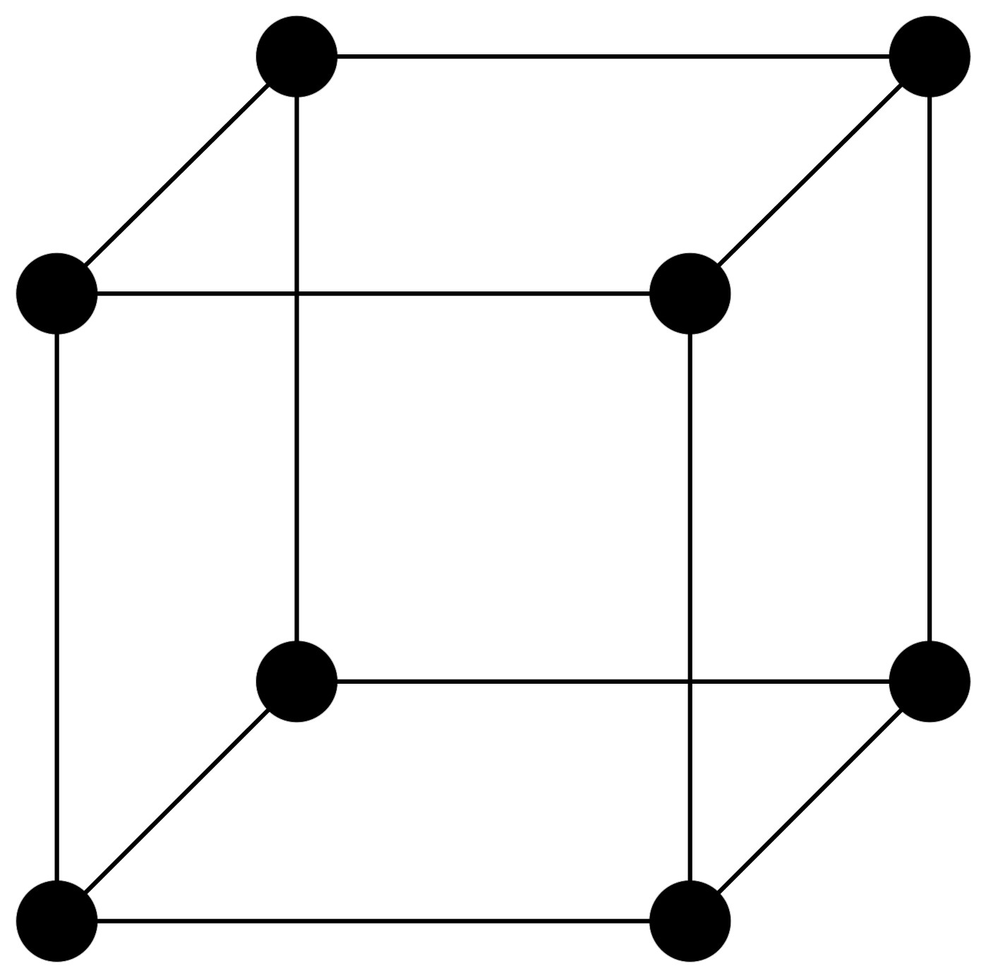
Figure 5 illustrates the five network structures we have chosen for our experiments.



Appendix B Effect of Network Structure
Communication matrix. We use the convention that a node is a neighbor of itself, i.e. . We assume that is doubly stochastic, i.e. if , and if and , and finally for every . It is known that the eigenvalues of a doubly stochastic matrix can be ordered in a descending manner satisfying , where the largest eigenvalue is with an all-one eigenvector. The eigenvalues of can be used to reveal the properties of the network associated with the weight matrix (see e.g. [Chung 1997]). A common approach is to take where is the identity, is the graph Laplacian and small enough [Olfati-Saber et al. 2007].
B.1 Examples
Adjacency matrix and degree matrix: For an undirected graph with nodes , an adjacency matrix is a symmetric matrix with if there is an edge between node and node and otherwise. The degree matrix of an undirected graph is a diagonal matrix with the diagonals counting the degrees of the nodes, more precisely, with the -th diagonal being . See e.g. [Chung 1997].
Graph Laplacian: The graph Laplacian for an undirected graph with nodes has the form
where is the degree matrix and is the adjacency matrix which is symmetric; see e.g. [Cvetkovć et al. 1998]. The eigenvalues of are non-negative: (see e.g. [Chung 1997]). For any , we take the communication matrix as:
| (B.1) |
It follows that is symmetric doubly stochastic with eigenvalues , where for any .
Complete graph with nodes: For the complete graph on vertices, the adjacency matrix , where and for any . One can compute that the Laplacian is where and for any . In this case, the communication matrix is given by
| (B.2) |
Star graph with nodes: For the star graph on vertices, the adjacency matrix , where and for any and for any . One can compute that the Laplacian is where , for any , and otherwise. In this case, the communication matrix is given by
| (B.3) |
Cycle graph with nodes: For the cycle graph on vertices, the adjacency matrix , where for any , and otherwise. One can compute that the Laplacian is where for any , and for any , , and otherwise. In this case, the communication matrix is given by
| (B.4) |
Hypercube graph with nodes: Consider the hypercube graph with nodes. The hypercube has adjacency matrix:
| (B.5) |
and the Laplacian matrix:
| (B.6) |
Bipartite graph with nodes: We consider the complete bipartite graph on vertices, where is an even integer whose vertices are divided into two equal size sets with vertices, and the adjacency matrix is given by
| (B.7) |
One can compute that the Laplacian is given by . In this case, the communication matrix is given by
| (B.8) |
Barbell graph with nodes: We consider the barbell graph on vertices, where is an even integer whose vertices are divided into two equal size sets with vertices, and the adjacency matrix is given by for any , for any , and otherwise. We can compute that the Laplacian is given by , where for any , for any , , , for any and otherwise.
Path graph with nodes: For the path graph (line graph) on vertices, the adjacency matrix , where for any and and otherwise. We can compute that the Laplacian is given by , where , for any , for any and and otherwise.
Appendix C Generalized Central Limit Theorem
In this section, by following Theorem 2, we derive a generalized central limit theorem (GCLT) as a corollary to [Gao et al. 2015, Theorem 1.1].
Before we state the next result, let us first recall -stable distributions from probability theory. The -stable distributions are heavy-tailed distributions that appear as the limiting distribution of the generalized CLT for a sum of i.i.d. random variables with infinite variance [Lévy 1937]. Here, is known as the tail-index, which determines the tail thickness of the distribution. An -stable distribution becomes heavier-tailed as gets smaller. When and , an -stable distribution reduces to the Cauchy and the Gaussian distributions, respectively.
In particular, the next result shows that, when properly scaled, the sum of the iterates converges in law to an -stable distribution.
Corollary 8.
Assume the conditions of Theorem 2 are satisfied, i.e. assume and there exists a unique positive such that . Then, there exists a function such that for , the random variables converge in law to the random variable with characteristic function , for and as .
Here, if , , ; if , , ; if , , ; finally, if , , , where .
The proof requires verifying that the conditions of [Gao et al. 2015, Theorem 1.1] hold under our assumptions. Similar to Theorem 2, the proof is a straightforward extension of the proof of [Gürbüzbalaban et al. 2021, Theorem 2], hence omitted. For , a similar GCLT holds with more complicated terms, which we omitted for brevity.
This result shows that, when , the scaled and centered sum converges to a Gaussian distribution (that is a -stable distribution); whereas when , the sequence converges to an -stable distribution, where coincides with the tail-index of the stable distribution as well.
Appendix D Moment Bounds and Convergence Speed
Wasserstein metric. For any , define as the space consisting of all the Borel probability measures on with the finite -th moment (based on the Euclidean norm). For any two Borel probability measures , we define the standard -Wasserstein metric [Villani 2009]:
where the infimum is taken over all joint distributions of the random variables with marginal distributions .
D.1 Moment Bounds
Theorem 2 is of asymptotic nature which characterizes the stationary distribution of SGD iterations. Next, we provide non-asymptotic moment bounds for at each -th iterate, and also for the limit . In the rest of Appendix D, we assume that
| (D.1) |
so that there exists a unique positive value such that . We have shown previously in Section 4 that a sufficient condition for (D.1) to hold is , and being sufficiently small.
Theorem 9.
Suppose Assumptions (A1)-(A2) hold.
(i) If the tail-index , then for any , we have and
| (D.2) |
(ii) If the tail-index , then for any , we have and for any , we have
| (D.3) |
By letting , we obtain the following corollary.
Corollary 10.
Suppose Assumptions (A1)-(A3) hold.
Suppose Assumptions (A1)-(A2) hold.
(i) If the tail-index , then for any , we have and
| (D.4) |
(ii) If the tail-index , then for any , we have and for any , we have
| (D.5) |
D.2 Convergence Speed
Next, we will study the speed of convergence of the -th iterate to its stationary distribution in the Wasserstein metric for any .
Theorem 11.
Suppose Assumptions (A1)-(A2) hold. Assume . Let , denote the probability laws of and respectively. Then for any ,
where .
We can see from Theorem 11 that converges exponentially fast in to with the convergence rate . Theorem 11 works for any . At the critical , by adapting the proof of Proposition 10 in Gürbüzbalaban et al. 2021, one can show the following result.
Proposition 12.
Suppose Assumptions (A1)-(A2) hold. Then we have if , and if .
Appendix E Tail-Index Comparison
E.1 Tail-Index Comparison between Decentralized SGD and Disconnected SGD: The General Case
In Section 4, we compared the tail-index between decentralized SGD and disconnected SGD for the special case when the dimension , the batch-sizes . In this section, we will discuss the general case.
E.1.1 General dimension , batch-sizes and variances
More generally, we consider the general dimension , batch-sizes and . Let and be the right and left singular vectors of the matrix , i.e. they satisfy
| (E.1) |
where
Then, we can choose the left and right eigenvectors of the matrix corresponding to the largest singular value
| (E.2) |
as
where is the index that maximizes in (E.2) and
is the index of the eigenvalues of so that we have
| (E.3) |
Basically, is the index of the node where is maximized whereas is the index of the eigenvalue of for which the 2-norm is attained (i.e. (E.3) is satisfied). For example, if and ; we have
where is the left eigenvector of and denotes the zero vector of length . As before,
| (E.4) |
where we used . In the special case when and , we have
so that we recover (F.19).
Lemma 13.
As , we have the first-order expansion:
| (E.5) |
where
| (E.6) |
In Lemma 13, we obtained the first-order approximation of in terms of , a correction term linear in , and a higher-order error term. Note that
and since are i.i.d. continuously distributed, such that when , with probability , the smallest eigenvalue of is such that and when , with probability , the smallest eigenvalue of is greater than , and hence we focus on the case and so that there exists a unique positive value such that and for sufficiently small, there exists a unique positive value such that . Next, we are going to utilize Lemma 13 to obtain a first-order approximation of the tail-index in terms of the tail-index , a correction term linear in and a higher-order error term.
Theorem 14.
Assume and . As , we have the first-order expansion:
| (E.7) |
We can see from Theorem 14 that the second term on the right hand side of (E.7) is positive if and only if , and this probability is monotonically decreasing in and . Therefore, we conclude from Theorem 14 that when is small, given the stepsize or network size is large. On the other hand, when is small, given the stepsize or network size is small.
Next, let us consider the special case and , under which we are able to obtain a more explicit characterization of the tail-index.
Theorem 15.
Assume . Also assume that . As , we have
| (E.8) |
where
| (E.9) |
and
| (E.10) |
where and are the probability density and cumulative distribution functions of .
In particular, when are i.i.d. distributed, we have the following corollary.
E.1.2 General dimension , batch-sizes and variances
More generally, we consider the general dimension , batch-sizes and variances . It follows from (E.4) that
| (E.12) |
where is the index that maximizes in (E.2) and
is the index of the eigenvalues of so that we have
| (E.13) |
Lemma 17.
As , we have the first-order expansion:
| (E.14) |
where
| (E.15) |
In Lemma 17, we obtained the first-order approximation of in terms of , a correction term linear in , and a higher-order error term. Note that
and since are continuously distributed, such that when , with probability , the smallest eigenvalue of is such that and when , with probability , the smallest eigenvalue of is greater than , and hence we focus on the case for every and so that there exists a unique positive value such that and for sufficiently small, there exists a unique positive value such that . Next, we are going to utilize Lemma 17 to obtain a first-order approximation of the tail-index in terms of the tail-index , a correction term linear in and a higher-order error term.
Theorem 18.
Assume for every and . As , we have the first-order expansion:
| (E.16) |
Next, let us consider the special case , under which we are able to obtain a more explicit characterization of the tail-index
Theorem 19.
Assume . Also assume that , where . As , we have
| (E.17) |
where
and
| (E.18) |
where are the probability density and probability distribution functions of .
In particular, when for every , are i.i.d. distributed, we have the following corollary.
E.2 Tail-Index Comparison between Decentralized SGD and Centralized SGD: The General Case
In this section, we are interested in comparing the tail-index for the DE-SGD with that of the C-SGD for the general dimension case where we assume and .
In Proposition 4, we showed that the tail-index for Dis-SGD is smaller than that of the C-SGD. In Theorem 14 we showed that when is small, the tail-index for the DE-SGD is small than that of the Dis-SGD given the stepsize or network size is large. Therefore, we have the following corollary that compares the tail-index for the DE-SGD with that of the C-SGD.
Corollary 21.
Under the assumptions in Theorem 14, the tail-index of the decentralized SGD is smaller than that of the centralized SGD provided that the stepsize or network size is large and is small.
On the other hand, we showed in Theorem 14 when is small, the tail-index for the DE-SGD is larger than that of the Dis-SGD given the stepsize or network size is small. Therefore, our theory (Proposition 4 and Theorem 14) does not provide a guidance to the comparison of the tail-indexes between DE-SGD and C-SGD in this regime. However, in the numerical experiments section, we have observed that DE-SGD lead to heavier tails than C-SGD.
Appendix F Technical Proofs
F.1 Proof of Results in Section 3
F.1.1 Proof of Proposition 1
We will first show that under the assumptions of Proposition 1, the function is strongly convex outside a compact region, and the result will follow from Hodgkinson and Mahoney 2021.
By assumption, the function is -strongly convex outside a compact region for some , therefore there exists such that the Hessian matrix whenever . For any given , consider the set
Notice that
For and with , we have for every by the definition of . Therefore,
with where we used the facts that is - strongly convex outside the compact ball of radius and we have for any .
It remains to show that for and , strong convexity also holds; i.e.
| (F.1) |
for some . Towards this direction, we start with a technical lemma.
Lemma 22.
For , we have
| (F.2) |
for some .
Proof.
Note that the eigenvalues of are each with multiplicity . Let
be the eigenvalues of in increasing order and let be an eigenvector of unit norm corresponding to the eigenvalue . Note that we have
and
Note that we can take for where 1 is the vector of ones of length and is the -th basis vector in .
To show (F.2), without loss of generality, assume .22 2 If this is not the case, we could apply the same proof technique to the normalized vector which will have unit norm). We introduce the -dimensional subspace:
| (F.3) |
We observe that and notice that is the null space of . We can also write in the basis of eigenvectors; i.e. we can write where . Since the eigenvectors and are orthogonal for , we have . We can also write
where and lies in the subspace orthogonal to . Since , we have also
| (F.4) |
where we used and for . Recalling that , to show (F.2), it suffices to show that for some .
Since by the assumption, we have such that
| (F.5) |
If we consider the optimization problem
| (F.6) |
It is easy to see from the right-hand side of (F.6) that the maximizer is
which yields the optimum value
Note that we have because by Cauchy-Schwarz inequality
| (F.7) |
and the equality is attained only when (and this cannot be the case due to (F.5)). In particular, we have
| (F.8) |
because the supremum is taken over a compact set and attained at a point with . Note that and is of the form with where . Therefore, we obtain from (F.6) and (F.8) that
Writing into this equation and using leads to
Equipped with this lemma, the stage is set for completing the proof of Proposition 1. Notice that by the continuity of the second derivatives, there exists a positive constant such that for every whenever . For , we have
for sufficiently small where we used Lemma 22. This proves (F.1). We conclude that for , we have for sufficiently small .
Based on this property, the results follow from [Hodgkinson and Mahoney 2021, Theorem 1 and Example 4]. This completes the proof.
F.2 Proof of Results in Section 4
F.2.1 Proof of Theorem 3
The follows by adapting the proof of Theorem 4 in Gürbüzbalaban et al. 2021 by working with the norm instead of the norm, where is the first basis vector.
F.2.2 Proof of Proposition 4
By adapting the proof of Theorem 4 in Gürbüzbalaban et al. 2021 to work with the norm instead of the norm, where is the first basis vector, we can show that as a function of the batch-size is increasing in . Thus . Moreover, is increasing in . Hence, the conclusion follows.
F.2.3 Proof of Theorem 5
Before we proceed to the proof of Theorem 5, let us first provide a complete statement with all the technical details.
Theorem 23 (Complete Statement of Theorem 5).
Assume and . Also assume that . As , we have
| (F.9) |
where we provide an explicit formula for the probability and the expectation on the right hand side of (F.9) as follows:
| (F.10) | ||||
| (F.11) |
where and are the probability density and cumulative distribution functions of .
Before we proceed to the proof of Theorem 5, let us first prove the following lemma, which provides a first-order expansion of . The proof of Theorem 5 will be then based on utilizing this lemma.
Lemma 24.
Assume and . Also assume that are i.i.d. with a continuous distribution. As , we have
| (F.12) |
where
| (F.13) |
and
| (F.14) |
where and are the probability density and cumulative distribution functions of .
Before we proceed to the proof of Lemma 24, let us first recall that
| (F.15) |
where:
| (F.16) |
In the following, we start with considering the Taylor series expansion of around : By the standard perturbation theory for singular values, we have
| (F.17) |
(see e.g. [Guglielmi and Overton 2011, Lemma 2.3]) where and are the left and right eigenvectors of satisfying
| (F.18) |
with where is the largest singular value of . Since is symmetric we can choose . Because of the block diagonal structure of , we have also
We recall that in Theorem 5 and Lemma 24, we take and , so that we have and is a scalar. Thus,
Let be the index for which the maximum on the right-hand side is attained. Then, we can choose the left and right eigenvectors and as
where denotes the sign function and is the -th basis vector. Indeed, it is easy to check that this choice of and satisfies (F.18) for . Then, by plugging this choice of and into (F.17), we obtain
We note . This implies
| (F.19) |
This shows that for sufficiently small , we have with high probability in which case we obtain
On the other hand, if is sufficiently large (or is sufficiently large) then with high probability in this case we obtain
We conclude that if the stepsize is very small, adding the network will increase the tail-index. whereas if the stepsize is large enough, adding the network will decrease the tail-index. We will next provide a rigorous proof of Lemma 24 to make this statement precise.
Proof of Lemma 24.
By taking the expectations in (F.19), we obtain
| (F.20) |
Notice that are i.i.d. distributed with a continuous distribution. Therefore, is uniformly distributed on and we can compute that
Moreover, we can compute that
and we can further compute that
where we recall that . It is easy to see that
| (F.21) |
and one can further deduce that
| (F.22) |
which is equivalent to
| (F.23) |
which holds if and only if
| (F.24) |
that is equivalent to
| (F.25) |
Hence, we conclude that
| (F.26) |
Note that are i.i.d. distributed with a continuous distribution. Let and be the probability density function and the cumulative distribution function of . By definition, . For any , we have
Let be the joint probability density function of and . Then, for any ,
This implies that
Hence, we conclude that
Now, we are ready to prove Theorem 5.
Under the assumption that , we have as well for sufficiently small . Thus, there exist unique positive values and such that and .
Let us write to emphasize the dependence on so that
| (F.27) |
Then we have . By differentiating with respect to , we obtain
| (F.28) |
We can compute from (F.27) that
We can further compute that
Notice that for any ,
where we recall that is the cumulative distribution function of . By differentiating with respect to , we obtain
where we recall that is the probability density function of . Hence, we conclude that
F.2.4 Proof of Corollary 6
Corollary 25 (Complete Statement of Corollary 6).
(i) Under the assumptions in Theorem 23, further assume that the stepsize . For sufficiently small , , i.e. the tail gets heavier with the presence of network effect. (ii) Further assume that are i.i.d. distributed. Then, as , we have the first-order expansion (4.1) with and in (F.10)-(F.11). Moreover, when the variance , for sufficiently small , , i.e. the tail gets heavier with the presence of network effect.
Now we are ready to prove Corollary 6.
(i) First, we notice that
| (F.30) |
since is the unique positive value such that and and and is convex in (see [Gürbüzbalaban et al. 2021]) so that .
For sufficiently small , if follows from Theorem 5 that if and only if
| (F.31) |
Note that a sufficient condition for (F.31) to hold is that
| (F.32) |
which is equivalent to
| (F.33) |
(ii) Let and be the probability density function and the cumulative distribution function of . In particular, when , we have for any , so that for any ,
| (F.34) |
and thus
| (F.35) |
where erf denotes the error function, i.e. . By applying Theorem 5, we conclude that as , we have the first-order expansion (4.1) with and in (F.10)-(F.11).
Finally, it follows from (i) and its proof that if
| (F.36) |
then, for sufficiently small , . When are i.i.d. distributed, the condition (F.36) is equivalent to
| (F.37) |
This completes the proof.
F.2.5 Proof of Corollary 7
F.3 Proofs of Results in Section D
F.3.1 Proof of Theorem 9
We adapt the proof of Theorem 6 in Gürbüzbalaban et al. 2021. We recall that
| (F.38) |
which implies that
| (F.39) |
(i) If the tail-index , then for any , we have and moreover by applying Lemma 23 in Gürbüzbalaban et al. 2021,
| (F.40) |
so that
with , where we used the fact that is independent of . By iterating over , we get
| (F.41) |
(ii) If the tail-index , then for any , by applying Lemma 23 in Gürbüzbalaban et al. 2021, for any , we have
| (F.42) |
which (similar as in (i)) implies that
| (F.43) |
We choose so that . By iterating over , we get
| (F.44) |
The proof is complete.
F.3.2 Proof of Theorem 11
We adapt the proof of Theorem 8 in Gürbüzbalaban et al. 2021. For any , there exists a couple and independent of and . We define and starting from and respectively, via the iterates
| (F.45) | ||||
| (F.46) |
and let and denote the probability laws of and respectively. For any , since and , we have for any . Moreover, we have
which by iterating implies that
| (F.47) |
By letting , the probability law of the stationary distribution , we conclude that
| (F.48) |
Finally, notice that , and therefore . The proof is complete.
F.4 Proofs of Results in Section E
F.4.1 Proof of Lemma 13
By taking the expectations in (E.4), we get
| (F.49) |
Note that are i.i.d. distributed, where are i.i.d. following a continuous distribution. Therefore, is uniformly distributed on and we can compute that
Moreover, we can compute that
and we can further compute that
and hence as , we have the first-order expansion:
| (F.50) |
where
| (F.51) |
which completes the proof.
F.4.2 Proof of Theorem 14
Under the assumption that , we have as well for sufficiently small . Thus, there exist unique positive values and such that and .
F.4.3 Proof of Theorem 15
When , we can compute that . Under the assumption that , we have as well for sufficiently small . Thus, there exist unique positive values and such that and .
When , we can compute that
Moreover, we can compute that
The rest of the proof follows similarly as in the proof of Theorem 5.
F.4.4 Proof of Corollary 16
When and are i.i.d. , we have
| (F.54) |
in distribution, where denotes a chi-square random variable with degrees of freedom and hence
| (F.55) |
and
| (F.56) |
where is the gamma function and is the lower incomplete gamma function. The proof is completed by applying Theorem 15.
F.4.5 Proof of Lemma 17
By taking the expectations, we get
| (F.57) |
and we can compute that
and hence as , we have the first-order expansion:
| (F.58) |
where
| (F.59) |
which completes the proof.
F.4.6 Proof of Theorem 18
Under the assumption that , we have as well for sufficiently small . Thus, there exist unique positive values and such that and .
F.4.7 Proof of Theorem 19
When , . Under the assumption that , we have as well for sufficiently small . Thus, there exist unique positive values and such that and .
When , . It is easy to see that
| (F.62) |
and one can further deduce that
| (F.63) |
which is equivalent to
| (F.64) |
which, by the similar argument as in the proof of Lemma 24, holds if and only if
| (F.65) |
Therefore, we can compute that
Let and be the probability density function and the cumulative distribution function of . For any , we have
Let be the joint probability density function of and . Then, for any ,
This implies that
Similarly,
Finally, we can compute that
Notice that for any ,
where we recall that is the cumulative distribution function of . By differentiating with respect to , we obtain
where we recall that is the probability density function of . This completes the proof.
F.4.8 Proof of Corollary 20
When , for every , are i.i.d. , we have
| (F.66) |
in distribution, where denotes a chi-square random variable with degrees of freedom and hence
| (F.67) |
and
| (F.68) |
where is the gamma function and is the lower incomplete gamma function. The proof is completed by applying Theorem 19.
F.4.9 Proof of Corollary 21
Appendix G Further experiments with synthetic data


Further Illustrations of Thm. 5 and Cor. 6
Due to space limit in the main text, we provide some of our experimental results in Figure 6. In the main text we have provided Figure 3(b), which fit into Case II () described in the numerical experiments section in the main text. Figure 6(a) and Figure 6(b) illustrate Case II as well. In Figure 6(a), we set and generate by simulating the model (5.1). We run the DE-SGD on the star network with and different value . For Figure 6(b), we set and run DE-SGD on the star network with . We can see that both Dis-SGD and DE-SGD will converge to a heavy-tailed distribution. In the small stepsize regime, Dis-SGD will have heavier tail, and in the big stepsize regime, DE-SGD will have heavier tail. Our observation is the same as our expectation.
Effect of parameters.
In this set of experiments, we investigate the tail-index of the stationary distribution of DE-SGD over different network topologies with varied stepsize and varied batch size . We set , , , and generate by simulating the model (5.1). To mimic the C-SGD, we run the single-node SGD in the same experimental setup but with batch-size . We consider 5 different network topologies in the experiments and take the communication matrix . They are (a) complete network with (b) cycle network with (c) hypercube network with (d) bipartite network with and (e) star network with . These networks and their basic properties are discussed in Section A and B.
First, we plot how the DE-SGD tail-index varies with stepsize from to for the five network topologies in Figure 7(a). We observe that The tail-index of DE-SGD over different topologies decreases as stepsizes increase and becomes heavy tailed when stepsize is larger than a threshold (threshold depends on the network structure). DE-SGD has heavier tails (smaller ) compared to C-SGD. This is also consistent with our Corollary 7. In another set of experiments, we investigate the tail-index of the stationary distribution of DE-SGD over different network topologies with varied batch-size . We set stepsize and vary batch-size from 1 to 8 for each node in DE-SGD. For C-SGD, we use a batch size of bN as is varied. The results are displayed in Figure 7(b). It is observed that Heavier tails occur for small batch-sizs, the larger batch size gets; we have lighter behavior ( corresponds to Gaussian tails). This is consistent with our result (Theorem 3) and also with the experiments of Panigrahi et al. 2019 in the centralized setting. The tail of the stationary distribution of DE-SGD over all topologies is always heavier than that of the C-SGD. This is in line with our Corollary 7.


Appendix H Tail index estimation in the numerical experiments
H.1 Synthetic data experiments
Both DE-SGD and C-SGD iterates converge to a stationary distribution with proper choice of parameters. By the generalized CLT result, the ergodic average of the iterates will converge to an -stable distribution where if the stationary distribution has infinite variance, otherwise. To estimate the tail index of the averaged iterates, we use the same approach proposed in Gürbüzbalaban et al. 2021. Basically, we run the DE-SGD recursion (2.1) with a random initial point for each node , and each entry in follows an i.i.d. uniform distribution . We repeat this procedure 1,600 times for different initial points and obtain 1,600 different random vectors for each node . After that, instead of using the estimator proposed by Mohammadi et al. 2015 that evaluates directly on the final iterate , building on the generalized CLT result, we compute the average of the ‘centered’ iterates , where is a ‘burn-in’ period aiming to discard the initial phase of the stochastic algorithms, and denotes the mean of the final iterates. We apply the estimator of Mohammadi et al. 2015 to the average of the ‘centered iterates’. In our synthetic experiments, we set .
H.2 Deep learning experiments
For estimating the tail index in the deep learning experiments, we use a similar approach to the one described in Section H.1. Basically, after training each neural network model sufficiently, we compute the average of the last 1000 algorithm iterates, whose distribution we expect to be close to an -stable distribution by the GCLT. We then treat each layer as a collection of i.i.d. -stable random variables and measure the tail-index of each individual layer separately by using the estimator from Mohammadi et al. 2015.
Appendix I Further Details of ResNet-20 Experiments
Due to space limit in the main text, we are reporting some of the details of our ResNet-20 experiments with nodes (corresponding to Figure 4(b) in the main text) in this section.
For the experiments in Figure 4(b), after the tail-index of each layer in the ResNet-20 model is estimated, we treat the median of them as the tail-index of the whole ResNet-20 model. We train the ResNet-20 model for 200 epochs. The learning rate is warmed up in the first 5 epochs and is decayed by a factor of 10 at the 100th and 150th epoch. We set the network size as and simulate all nodes with three 2080Ti GPUs (each GPU simulates 8 nodes). Moreover, each node samples data per iteration. Since this experiment is on a real distributed GPU system, we utilize BlueFog [Ying et al. 2021b] for the implementation of decentralized methods including topology organization, weight matrix generation, and efficient decentralized communication. For the implementation of C-SGD, we utilize PyTorch’s native Distributed Data Parallel (DDP) module. All algorithms are tested with stepsizes ranging from 0.025 to 0.2. We find stepsizes larger than 0.2 will cause significant performance dropping in test accuracy.

Besides the experiment for shown in Figure 4(b), we also report the results of our experiments for in Figure 8, where all other settings are the same as in Figure 4(b). We can see that for the case, the tail-index of DE-SGD and C-SGD are closer to each other, whereas for case, the tail-index difference between DE-SGD and C-SGD is clearer. This suggests that we can observe the phenomenon that DE-SGD has heavier tail than C-SGD, and the phenomenon will be clearer when the size of network gets larger. In fact, Proposition 4 shows that the difference between the tail indices of Dis-SGD and C-SGD gets larger as increases, and our numerical results are compatible with this theoretical result.